
In some cases, numbers in a worksheet are actually formatted and stored in cells as text, which can cause problems with calculations or produce confusing sort orders. This issue sometimes occurs after you import or copy data from a database or other external data source.
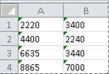
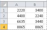
Numbers that are formatted as text are left-aligned instead of right-aligned in the cell, and are often marked with an error indicator.
What do you want to do?
-
Technique 1: Convert text-formatted numbers by using Error Checking
-
Technique 2: Convert text-formatted numbers by using Paste Special
-
Technique 3: Apply a number format to text-formatted numbers
-
Turn off Error Checking
Technique 1: Convert text-formatted numbers by using Error Checking
If you import data into Excel from another source, or if you type numbers into cells that were previously formatted as text, you may see a small green triangle in the upper-left corner of the cell. This error indicator tells you that the number is stored as text, as shown in this example.
If this isn’t what you want, you can follow these steps to convert the number that is stored as text back to a regular number.
-
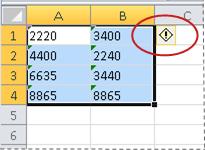
On the worksheet, select any single cell or range of cells that has an error indicator in the upper-left corner.
How to select cells, ranges, rows, or columns
To select
Do this
A single cell
Click the cell, or press the arrow keys to move to the cell.
A range of cells
Click the first cell in the range, and then drag to the last cell, or hold down Shift while you press the arrow keys to extend the selection.
You can also select the first cell in the range, and then press F8 to extend the selection by using the arrow keys. To stop extending the selection, press F8 again.
A large range of cells
Click the first cell in the range, and then hold down Shift while you click the last cell in the range. You can scroll to make the last cell visible.
All cells on a worksheet
Click the Select All button.

To select the entire worksheet, you can also press Ctrl+A.
If the worksheet contains data, Ctrl+A selects the current region. Pressing Ctrl+A a second time selects the entire worksheet.
Nonadjacent cells or cell ranges
Select the first cell or range of cells, and then hold down Ctrl while you select the other cells or ranges.
You can also select the first cell or range of cells, and then press Shift+F8 to add another nonadjacent cell or range to the selection. To stop adding cells or ranges to the selection, press Shift+F8 again.
You cannot cancel the selection of a cell or range of cells in a nonadjacent selection without canceling the entire selection.
An entire row or column
Click the row or column heading.
1. Row heading
2. Column heading
You can also select cells in a row or column by selecting the first cell and then pressing Ctrl+Shift+Arrow key (Right Arrow or Left Arrow for rows, Up Arrow or Down Arrow for columns).
If the row or column contains data, Ctrl+Shift+Arrow key selects the row or column to the last used cell. Pressing Ctrl+Shift+Arrow key a second time selects the entire row or column.
Adjacent rows or columns
Drag across the row or column headings. Or select the first row or column; then hold down Shift while you select the last row or column.
Nonadjacent rows or columns
Click the column or row heading of the first row or column in your selection; then hold down Ctrl while you click the column or row headings of other rows or columns that you want to add to the selection.
The first or last cell in a row or column
Select a cell in the row or column, and then press Ctrl+Arrow key (Right Arrow or Left Arrow for rows, Up Arrow or Down Arrow for columns).
The first or last cell on a worksheet or in a Microsoft Office Excel table
Press Ctrl+Home to select the first cell on the worksheet or in an Excel list.
Press Ctrl+End to select the last cell on the worksheet or in an Excel list that contains data or formatting.
Cells to the last used cell on the worksheet (lower-right corner)
Select the first cell, and then press Ctrl+Shift+End to extend the selection of cells to the last used cell on the worksheet (lower-right corner).
Cells to the beginning of the worksheet
Select the first cell, and then press Ctrl+Shift+Home to extend the selection of cells to the beginning of the worksheet.
More or fewer cells than the active selection
Hold down Shift while you click the last cell that you want to include in the new selection. The rectangular range between the active cell and the cell that you click becomes the new selection.
To cancel a selection of cells, click any cell on the worksheet.
-
Next to the selected cell or range of cells, click the error button that appears.
-
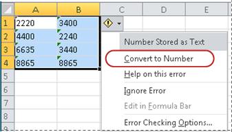
On the menu, click Convert to Number. (If you want to simply get rid of the error indicator without converting the number, click Ignore Error.)
This action converts the numbers that are stored as text back to numbers.
Once you have converted the numbers formatted as text into regular numbers, you can change the way the numbers appear in the cells by applying or customizing a number format. For more information, see Available number formats.

Top of Page
Technique 2: Convert text-formatted numbers by using Paste Special
In this technique, you multiply each selected cell by 1 in order to force the conversion from a text-formatted number to a regular number. Because you’re multiplying the contents of the cell by 1, the result in the cell looks identical. However, Excel actually replaces the text-based contents of the cell with a numerical equivalent.
-
Select a blank cell and verify that its number format is General.
How to verify the number format
-
On the Home tab, in the Number group, click the arrow next to the Number Format box, and then click General.
-
-
In the cell, type 1, and then press ENTER.
-
Select the cell, and then press Ctrl+C to copy the value to the Clipboard.
-
Select the cells or ranges of cells that contain the numbers stored as text that you want to convert.
How to select cells, ranges, rows, or columns
To select
Do this
A single cell
Click the cell, or press the arrow keys to move to the cell.
A range of cells
Click the first cell in the range, and then drag to the last cell, or hold down Shift while you press the arrow keys to extend the selection.
You can also select the first cell in the range, and then press F8 to extend the selection by using the arrow keys. To stop extending the selection, press F8 again.
A large range of cells
Click the first cell in the range, and then hold down Shift while you click the last cell in the range. You can scroll to make the last cell visible.
All cells on a worksheet
Click the Select All button.
To select the entire worksheet, you can also press Ctrl+A.
If the worksheet contains data, Ctrl+A selects the current region. Pressing Ctrl+A a second time selects the entire worksheet.
Nonadjacent cells or cell ranges
Select the first cell or range of cells, and then hold down Ctrl while you select the other cells or ranges.
You can also select the first cell or range of cells, and then press Shift+F8 to add another nonadjacent cell or range to the selection. To stop adding cells or ranges to the selection, press Shift+F8 again.
You cannot cancel the selection of a cell or range of cells in a nonadjacent selection without canceling the entire selection.
An entire row or column
Click the row or column heading.
1. Row heading
2. Column heading
You can also select cells in a row or column by selecting the first cell and then pressing Ctrl+Shift+Arrow key (Right Arrow or Left Arrow for rows, Up Arrow or Down Arrow for columns).
If the row or column contains data, Ctrl+Shift+Arrow key selects the row or column to the last used cell. Pressing Ctrl+Shift+Arrow key a second time selects the entire row or column.
Adjacent rows or columns
Drag across the row or column headings. Or select the first row or column; then hold down Shift while you select the last row or column.
Nonadjacent rows or columns
Click the column or row heading of the first row or column in your selection; then hold down Ctrl while you click the column or row headings of other rows or columns that you want to add to the selection.
The first or last cell in a row or column
Select a cell in the row or column, and then press Ctrl+Arrow key (Right Arrow or Left Arrow for rows, Up Arrow or Down Arrow for columns).
The first or last cell on a worksheet or in a Microsoft Office Excel table
Press Ctrl+Home to select the first cell on the worksheet or in an Excel list.
Press Ctrl+End to select the last cell on the worksheet or in an Excel list that contains data or formatting.
Cells to the last used cell on the worksheet (lower-right corner)
Select the first cell, and then press Ctrl+Shift+End to extend the selection of cells to the last used cell on the worksheet (lower-right corner).
Cells to the beginning of the worksheet
Select the first cell, and then press Ctrl+Shift+Home to extend the selection of cells to the beginning of the worksheet.
More or fewer cells than the active selection
Hold down Shift while you click the last cell that you want to include in the new selection. The rectangular range between the active cell and the cell that you click becomes the new selection.
To cancel a selection of cells, click any cell on the worksheet.
-
On the Home tab, in the Clipboard group, click the arrow below Paste, and then click Paste Special.
-
Under Operation, select Multiply, and then click OK.
-
To delete the content of the cell that you typed in step 2 after all numbers have been converted successfully, select that cell, and then press DELETE.
Some accounting programs display negative values as text, with the negative sign (–) to the right of the value. To convert the text string to a value, you must use a formula to return all the characters of the text string except the rightmost character (the negation sign), and then multiply the result by –1.
For example, if the value in cell A2 is «156–» the following formula converts the text to the value –156.
|
Data |
Formula |
|
156- |
=Left(A2,LEN(A2)-1)*-1 |
Top of Page
Technique 3: Apply a number format to text-formatted numbers
In some scenarios, you don’t have to convert numbers stored as text back to numbers, as described earlier in this article. Instead, you can just apply a number format to achieve the same result. For example, if you enter numbers in a workbook, and then format those numbers as text, you won’t see a green error indicator appear in the upper-left corner of the cell. In this case, you can apply number formatting.
-
Select the cells that contain the numbers that are stored as text.
How to select cells, ranges, rows, or columns
To select
Do this
A single cell
Click the cell, or press the arrow keys to move to the cell.
A range of cells
Click the first cell in the range, and then drag to the last cell, or hold down Shift while you press the arrow keys to extend the selection.
You can also select the first cell in the range, and then press F8 to extend the selection by using the arrow keys. To stop extending the selection, press F8 again.
A large range of cells
Click the first cell in the range, and then hold down Shift while you click the last cell in the range. You can scroll to make the last cell visible.
All cells on a worksheet
Click the Select All button.
To select the entire worksheet, you can also press Ctrl+A.
If the worksheet contains data, Ctrl+A selects the current region. Pressing Ctrl+A a second time selects the entire worksheet.
Nonadjacent cells or cell ranges
Select the first cell or range of cells, and then hold down Ctrl while you select the other cells or ranges.
You can also select the first cell or range of cells, and then press Shift+F8 to add another nonadjacent cell or range to the selection. To stop adding cells or ranges to the selection, press Shift+F8 again.
You cannot cancel the selection of a cell or range of cells in a nonadjacent selection without canceling the entire selection.
An entire row or column
Click the row or column heading.
1. Row heading
2. Column heading
You can also select cells in a row or column by selecting the first cell and then pressing Ctrl+Shift+Arrow key (Right Arrow or Left Arrow for rows, Up Arrow or Down Arrow for columns).
If the row or column contains data, Ctrl+Shift+Arrow key selects the row or column to the last used cell. Pressing Ctrl+Shift+Arrow key a second time selects the entire row or column.
Adjacent rows or columns
Drag across the row or column headings. Or select the first row or column; then hold down Shift while you select the last row or column.
Nonadjacent rows or columns
Click the column or row heading of the first row or column in your selection; then hold down Ctrl while you click the column or row headings of other rows or columns that you want to add to the selection.
The first or last cell in a row or column
Select a cell in the row or column, and then press Ctrl+Arrow key (Right Arrow or Left Arrow for rows, Up Arrow or Down Arrow for columns).
The first or last cell on a worksheet or in a Microsoft Office Excel table
Press Ctrl+Home to select the first cell on the worksheet or in an Excel list.
Press Ctrl+End to select the last cell on the worksheet or in an Excel list that contains data or formatting.
Cells to the last used cell on the worksheet (lower-right corner)
Select the first cell, and then press Ctrl+Shift+End to extend the selection of cells to the last used cell on the worksheet (lower-right corner).
Cells to the beginning of the worksheet
Select the first cell, and then press Ctrl+Shift+Home to extend the selection of cells to the beginning of the worksheet.
More or fewer cells than the active selection
Hold down Shift while you click the last cell that you want to include in the new selection. The rectangular range between the active cell and the cell that you click becomes the new selection.
To cancel a selection of cells, click any cell on the worksheet.
-
On the Home tab, in the Number group, click the Dialog Box Launcher next to Number.
-
In the Category box, click the number format that you want to use.
For this procedure to complete successfully, make sure that the numbers that are stored as text do not include extra spaces or nonprintable characters in or around the numbers. The extra spaces or characters sometimes occur when you copy or import data from a database or other external source. To remove extra spaces from multiple numbers that are stored as text, you can use the TRIM function or CLEAN function. The TRIM function removes spaces from text except for single spaces between words. The CLEAN function removes all nonprintable characters from text.

Top of Page
Turn off Error Checking
With error checking turned on in Excel, you see a small green triangle if you enter a number into a cell that has text formatting applied to it. If you don’t want to see these error indicators, you can turn them off.
-
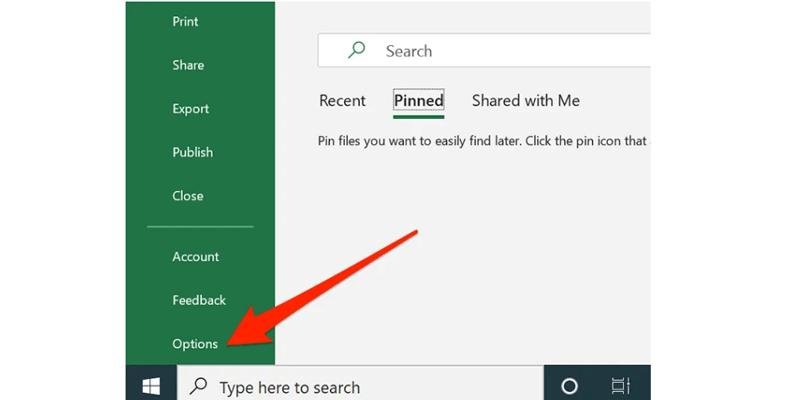
Click the File tab.
-
Under Help, click Options.
-
In the Excel Options dialog box, click the Formulas category.
-
Under Error checking rules, clear the Numbers formatted as text or preceded by an apostrophe check box.
-
Click OK.
Top of Page
Summary: Formatting issues in Excel are common that result in data loss and impede businesses. These Excel issues require proper and correct troubleshooting so that the data in the Excel files is meaningful and usable. Read on to know specific methods to fix the various Excel formatting issues.

A formatting issue in Excel may affect fonts, charts, shading, colors, borders, number formats, file formats, cell formats, hyperlink formats, and several other elements. For each of these different Excel format issues — Font Type and Size changed, Chart formatting, Conditional Formatting Rules, Text formatted to Number, Number formatted to Text or Date, Dates formatted to Numbers, etc. there are specific solutions.
A few common Excel formatting issues and how to fix them
- Date Format issue in Excel:
The typed-in date changes to a number, text, another format of date (for example, MM/DD/YYYY may change to DD/MM/YYYY), or any other format that Excel does not recognize.
An example of Excel Date Format issue is as follows:
A user enters or types a Date — September 6 in a cell of Excel file. However, on pressing the ‘Enter’ key the value of the cell converts to a ‘Number.’
This implies that the cell’s number format is not in sync with what the user is trying to achieve. The cell is set to the Number format, which converts the input to a numerical value.
Solution: Right-click the cell containing the Date, select ‘Format Cells’, click ‘Date’ present under Number à Category and finally choose a Date format of choice (Example: DD/MM/YYYY format).
Note – This is valid for older versions of Excel.

In Excel 2007 and above versions; click a cell, next click the drop-down arrow in the Number section of the Home tab. In doing so, a list of the Number format appears, along with the data represented in each of the formats.
- Number Format Issue and how to fix it
The Number format issue in Excel is an issue wherein a Number is formatted or changed to Text, Date, or any other format that is not recognized by Excel.
Solution: In such cases, users can use Error Checking or Paste Special as fixes.

- Formatting issues in font type, size, color, and conditional formatting:
These generally occur in Excel if users open Excel files on a system other than where those were created, or if the new system runs an older Office/Excel version.
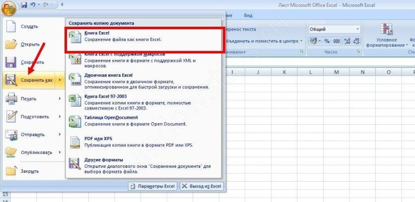
Solution: Users should make sure they save the Excel files in the native and widely accepted Excel 2007/2010 format, and not in the older Excel 97-2003 format. These are the options that users get while saving the Excel file using ‘Save As’ feature.

Users can also try to fix the Excel formatting issue by transferring all data from the current spreadsheet or workbook to a new and usable Excel workbook.
- Excel XLS or XLSX file corruption:
In such situations, the Excel files need to be repaired which can be done by using either the inbuilt ‘Open or Repair’ utility or an Excel file repair software such as Stellar Repair for Excel.
The software repairs the damaged Excel (XLS or XLSX) file in 3 quick and easy steps: Select, Scan, and Save. You can save the repaired file either at the default or desired location.
Conclusion
Despite being an amazing application that allows users to create and process complex data in workbooks. Microsoft Excel is not free from concerns including the ones that arise due to formatting issues. This is true for all Excel versions, be it the latest Excel 2016 or other lower versions. Therefore, the need to employ the appropriate fixes whenever required.
In addition, the use of an advanced Excel repair tool is recommended to fix issues that appear due to Excel file corruption. An advanced software such as Stellar Repair for Excel recovers the lost formatting from corrupt Excel files. It offers an intuitive interface to repair Font formatting, Chart Formatting, Conditional formatting rules and more while preserving the data format at the time of restoring the Excel files.
About The Author
Priyanka
Priyanka is a technology expert working for key technology domains that revolve around Data Recovery and related software’s. She got expertise on related subjects like SQL Database, Access Database, QuickBooks, and Microsoft Excel. Loves to write on different technology and data recovery subjects on regular basis. Technology freak who always found exploring neo-tech subjects, when not writing, research is something that keeps her going in life.
Best Selling Products

Stellar Repair for Excel
Stellar Repair for Excel software provid
Read More

Stellar Toolkit for File Repair
Microsoft office file repair toolkit to
Read More

Stellar Repair for QuickBooks ® Software
The most advanced tool to repair severel
Read More

Stellar Repair for Access
Powerful tool, widely trusted by users &
Read More
Формат ячейки не меняется в Excel? Скопируйте все разделы, в которых форматирование прошло гладко, выберите «плохие» области, щелкните их правой кнопкой мыши (ПКМ), затем «Специальная вставка» и «Форматы». Есть несколько других способов решения проблемы. Ниже мы рассмотрим, почему возникает такая ошибка, и проанализируем методы ее самостоятельного решения.
Для начала нужно понять, почему формат ячеек в Excel не меняется, чтобы найти эффективный метод решения проблемы. По умолчанию, когда вы вводите номер в бизнес-документ, он выравнивается по правому краю, а тип / размер определяется настройками системы.

Одна из причин, по которой в Excel не меняется формат ячеек, — это возникновение конфликта в этой области, из-за которого стиль заблокирован. В большинстве случаев проблема касается документов в Excel 2007 и других форматах. Часто это происходит из-за того, что новые форматы документов содержат информацию о форматировании ячеек в схеме XML, и иногда при редактировании возникает конфликт стилей. Excel, в свою очередь, не может быть установлен и, как следствие, не меняется.
Это лишь одна из причин, по которой формат не работает в Excel, но в большинстве случаев это единственное объяснение. Люди, столкнувшиеся с такой проблемой, часто не могут определить, когда она появилась. Учитывая ситуацию, есть несколько способов решения проблемы.
Что делать
В ситуации, когда формат ячеек в Excel не меняется, попробуйте один из следующих способов. Если метод вдруг не сработает, попробуйте другой вариант. Продолжайте, пока проблема не будет полностью решена.
Вариант №1
Во-первых, давайте рассмотрим один из наиболее эффективных способов решения этой проблемы в Excel. Алгоритм следующий:
- Проверьте, в каком формате сохранена книга. Если вы используете XLS, щелкните Сохранить как и книгу Excel (* .xlsx). Иногда ничего не меняется из-за неправильного расширения.
- Закройте документ.
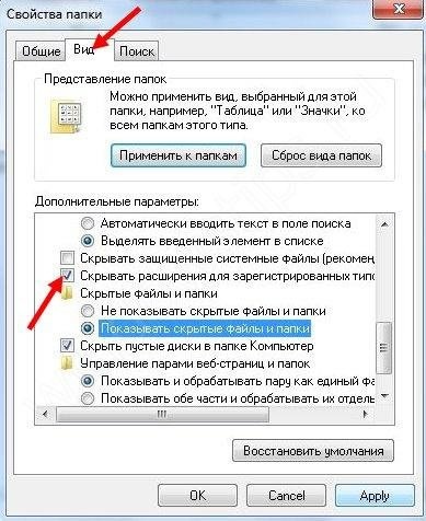
- Измените расширение книги с RAR на ZIP. Если расширение не отображается, перейдите в «Панель управления», затем «Свойства / Параметры папки», вкладку «Просмотр». Здесь снимите флажок «Скрыть расширение для зарегистрированных типов файлов».
- Откройте архив любой специальной программой.
- Найдите в нем следующие папки: _rels, docProps и xl.
- Войдите в xl и удалите Styles.xml.
- Закройте архив.
- Измените разрешение на основной .xlsx.
- Открываем книгу и соглашаемся на восстановление.
- Получите информацию об удаленных стилях, которые не удалось восстановить.
Затем сохраните книгу и проверьте, меняется ли форматирование ячеек в Excel. При использовании этого метода помните, что удаляются все форматы ячеек, включая те, с которыми ранее не возникало проблем. Информация о стиле шрифта, цвете, заливке, границах и т.д. Удаляется
Этот вариант наиболее эффективен, когда формат ячеек в Excel не меняется, но из-за его «массового» использования в будущем могут возникнуть трудности с настройкой. С другой стороны, риск возникновения такой же ошибки в будущем сводится к минимуму.
Вариант №2
Если формат ячейки внезапно не меняется в Excel, вы можете использовать другой метод:
- Скопируйте любую ячейку, с которой в этом вопросе не возникло затруднений.
- Используйте ПКМ, чтобы отбелить проблемный участок, на котором возникла проблема.
- Выберите Специальная вставка и форматы».
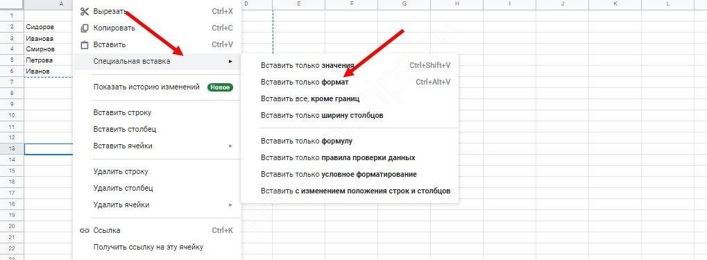
Этот метод хорошо работает, когда Excel не меняет формат ячеек, хотя раньше эта проблема не возникала. Его главное преимущество перед первым способом заключается в том, что остальные настройки сохраняются и не требуют сброса. Но есть одна особенность, которую следует отметить. Нет никакой гарантии, что сбой Excel не повторится в будущем.
Вариант №3
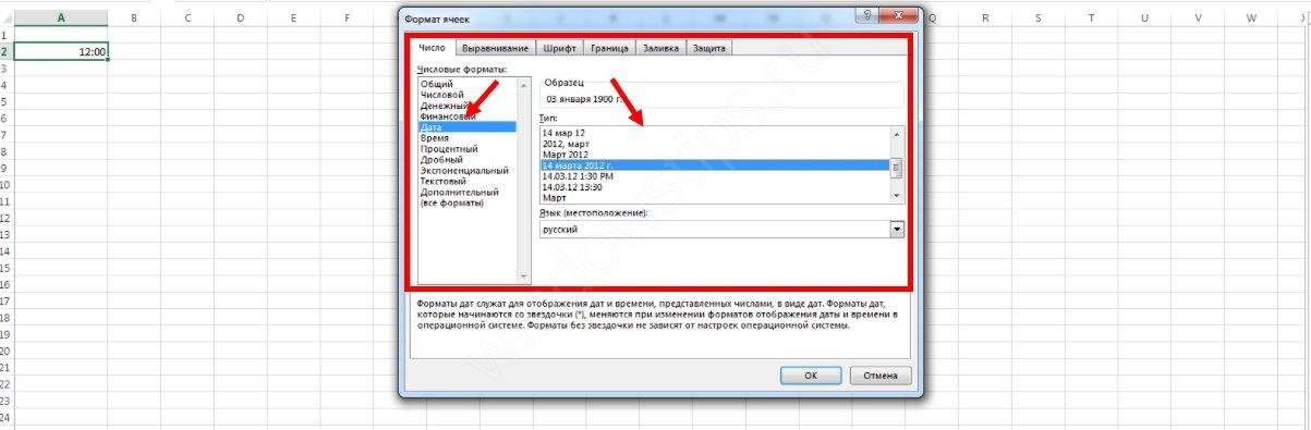
Следующее решение, когда форматирование в Excel не меняется, — попытаться выполнить работу правильно. Сделайте следующее:
- Выделите ячейки для форматирования.
- Нажмите Ctrl + 1.
- Введите «Формат ячеек» и откройте раздел «Число».
- Перейдите в раздел «Категория» и на следующем шаге — «Дата».
- В группе «Тип» выберите соответствующий формат информации. Будет возможность предварительно просмотреть формат с самой ранней датой в данных. Его можно найти в поле «Образец».
Чтобы быстро изменить форматирование даты по умолчанию, щелкните нужную область с датой, затем нажмите комбинацию Ctrl + Shift+#.
Вариант №4
Следующее решение, когда Excel не меняет формат ячеек, — попытаться установить правильный режим работы. Алгоритм действий следующий:
- Щелкните любой раздел с номером и нажмите комбинацию Ctrl + C.
- Выделите диапазон для преобразования.
- На вкладке «Вставка» нажмите «Специальная вставка».
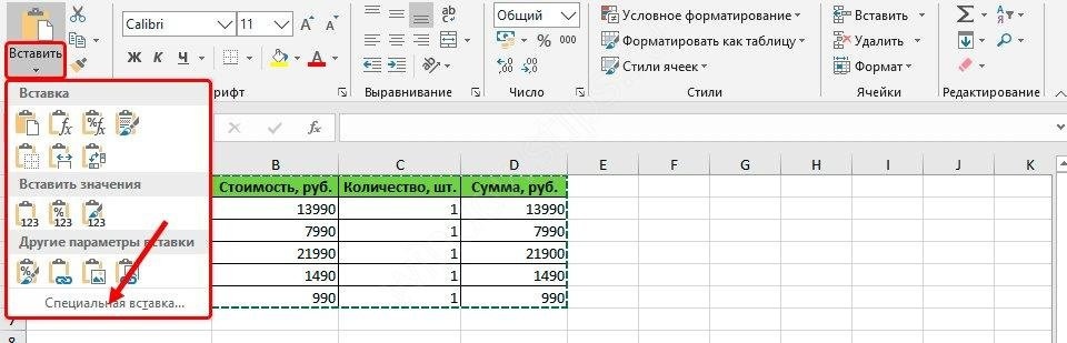
- В столбце «Операция» нажмите «Умножить».

- Выберите «ОК».
После этого попробуйте, вариант формата изменится по вашему запросу или неисправность останется в предыдущем режиме.
Вариант №5
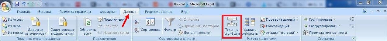
Иногда возникают ситуации, когда возникает проблема при сохранении отчета в Excel из 1С. После выделения столбца с числами и попытки выбрать формат чисел с разделителями и десятичными знаками ничего не меняется. В этом случае вам придется несколько раз щелкнуть по интересующей области.
Чтобы исправить это, сделайте следующее:
- Выделите весь столбец.
- Щелкните «Данные», затем «Текст по столбцам».
- Щелкните кнопку «Готово».
- Примените интересующее вас форматирование.
Как видите, техник достаточно, чтобы исправить ситуацию с форматом ячеек в Excel, когда он не меняется по команде. Для начала попробуйте первые два варианта, которые в большинстве случаев помогут решить проблему.
Receiving Excel file format and extension don’t match. the file could be corrupted or unsafe error? In that case this blog is going to be super beneficial for you. As it covers all the necessary details regarding Excel file format and extension don’t match error and ways to troubleshoot this on your own.
Before approaching the fixes let’s know about the reasons behind this Excel File Format And Extension error.
What Are The Causes Of ‘File Format And Extension Of Don’t Match’ Error?
Knowledge about the reasons for this file format and extension don’t match when opening Excel errors is important to apply the right solution.
- Wrong Extension –
This specific error mainly occurs because of the wrong or different extension. This scenario arise either when the file is converted to some other format or due to user’s manual intervention.
- Excel File Is Blocked –
In the Downloaded file of email attachments chances are high that properties levels are set blocked. As most of the email senders keep the properties blocked just for the sake of security purposes. So this is also one of the reasons behind why Excel file could be corrupted or unsafe error.
- File’s Incompatibility With Excel –
Another reason can be that the file which you are trying to access is not incompatible with your Excel application.
- Protected Views is Enabled –
Presence of a security option in your PC may be preventing the Excel application from opening certain files received through mail.
Below are some best applicable fixes to resolve Excel file and extensions that don’t match error.
Solution 1# Changing The Extension Manually
As through the error message you all must have noted that something went wrong in the Excel File Format and Extension. Maybe the Excel file which you are trying to open is in some different extension or unsupported format.
So to fix this you must try changing the extension of your Excel file to some other format.
Here is the quick guide on how to apply this step:
- First, go to the File Explorer and hit the View tab.
- Now from the opened menu bar, go to the show/hide group. Within this group there is an option File Name Extensions, put a check mark across that.

- After enabling the file name extension, go to the location where you have saved your error showing Excel file.
- Make a right click over that file and select the rename option.
- Change the extension to any of these formats: .xls or .xlsx or .xlsm and after every modification try to open your file.
In this way you will get the correct format which can easily open your Excel file without showing any error message.
Solution 2# Disable Add-ins
1: Press CTRL key from your keyboard and along with that tap to the Excel application icon. Very soon a confirmation dialog box will pop-up that will ask you to start your application in Safe mode.
2: If even after starting the application in safe mode, the problem persists then close your Excel application. Now start your application normally and try disabling the add-ins one by one.
3: Follow these paths to disable the add-ins: File > Options tab.
4: In the opened window of Excel options, go to the left pane and hit the Add-ins tab.
5: Now hit the Go button present beside the Manage: Excel Add-ins.

6: After that from the appearing list of Add-ins, uncheck each of the add-ins one by one to disable it.
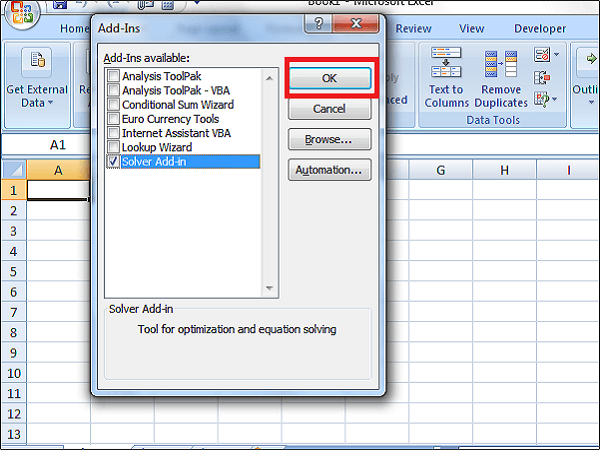
It’s time to check whether the problem has been resolved or not.
Solution 3# Unblocking The File
Excel file format and Extension of don’t match error also originates because it is blocked at properties level. Usually this problem is associated with receiving through email attachments or downloaded files on the internet.
This problem can be easily fixed by optimizing the file’s properties to unblock it.
Follow the below given steps to unblock Excel file:
- Make a right click over the error showing Excel file and choose the properties option.

- Now in the opened properties window move your cursor down here you will get the security section and then hit the “unblock” button.
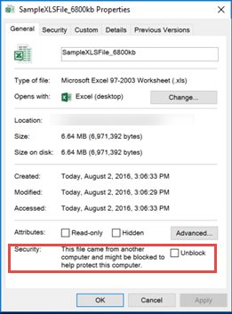
- After this step your Excel is now unblocked. So try re-opening your Excel file and check whether this time the problem is resolved or not.
If still you are getting the same Excel file extension won’t match error then move on to our next solution.
Solution 4# Open And Repair Inbuilt Tool
Open and repair inbuilt tool is the best option to resolve minor corruption or issues occurring in Excel files.
- Hit the file tab and choose the open option.

- Make a selection of the Excel file in which you are frequently getting this error.
- Now hit the arrow sign present next to the open Now from the drop-down menu choose the open and repair option.

- After that hit the repair button.

- If in case, this repair solution won’t fix the issue then repeat the above steps and hit the “Extract Data” option.

- In this way you can very easily extract data from your Excel file.
Solution 5# Disable The Protected View
File extension don’t match error also occurs when some new security option like protected view prevents the opening of certain Excel files.
Mainly such type of issue arises with the Excel files which were received through the email attachments.
Well this security setting can be easily cracked by disabling the protected view feature. So, here are the steps that you should follow to disable the Protected View setting.
- Open your Excel application.
- Hit the File> options tab.
- This will open the Excel options settings window.

- From the left side navigation pane, choose the Trust-center tab.
- Now from the opened window hit the Trust Center Settings.
- On the left side of the Trust Center window, you have chosen the Protected View.

- After that unselect all the previously selected options present within the protected view.

- Hit the Ok button to close the window.
Solution 6# Suppress The Error Warning Message
Another alternative option that you can try to fix Excel file format and extension of don’t match error is by creating the registry key to suppress this warning error message.
Note: making changes in the system registry setting is a bit risky and it can put your PC in a cumbersome situation.
Here is the quick guide on how you can suppress this file format and extension of don’t match error in Excel through the usage of registry editor:
- Hit Windows + R key together this will open the dialog box of Run.
- In this Run box, enter the text ‘regedit’ and hit the Enter button. This will open the Registry Editor.
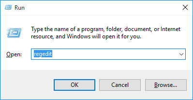
- Now in the prompt box opened through UAC (User Account Control), you need to hit the yes button.
- After getting into the Registry Editor utility, go to the right side pane and search for the following path.

HKEY_CURRENT_USERSoftwareMicrosoftOffice*X*ExcelSecurity
Note: as an alternative option you can also copy paste this location on the navigation bar and hit the enter button.
In the above given path” x” is to be replaced with your currently installed MS Office version.
- After getting into the correct location, shift to the right-side pane, and make a right-click over the empty space. Choose “NEW” and then “Dword (32-bit) value”.
- Name this DWORD value as Extension Hardening. After that, double-tap over it.
- Now set the Base as Hexadecimal and value as 0.
- Once you complete all these changes, shut down the Registry Editor and give a restart to your PC.
After the fresh start of the system you won’t get this annoying Excel error message.
Solution 7# Fix Excel File Corruption
If you are still getting the file format and extensions don’t match when opening Excel error then it’s recommended to use MS Excel Repair Tool. This is the best tool to fix any sort of issues, corruption, errors in Excel workbooks.
So if you are getting this error because of Excel file damage or corruption issues then this tool will surely resolve it.
With the help of this tool, you can easily restore all corrupt Excel files including the charts, worksheet properties, cell comments, and other important data. This is a unique tool to repair multiple Excel files at one repair cycle and recovers the entire data in a preferred location.
Steps To Repair Corrupt Excel File:
Solution 8# Open Excel File Without Excel
If your Excel file is refusing to open because of the file format or extension issue then you can try to open it using 3rd party apps. Yes, there are so many alternative options available to open Excel files without Excel.
Here are the following options using which you can easily perform this task: Chrome Browser’s Free Extension; Excel Viewer, Apache Open Office and many more.
Final Verdict:
Now you can fix Excel file format extension doesn’t match the error on your own. But make sure to follow the given fixes very carefully.
Moreover, feel free to run the Excel repair tool, to fix any type of internal issues and errors that might be causing the error in your Excel file.
If I missed out on any solution on how to fix Excel file format and extensions don’t match error. Or if you have any other trick to share, then do share it with us on our Facebook page.


Priyanka is an entrepreneur & content marketing expert. She writes tech blogs and has expertise in MS Office, Excel, and other tech subjects. Her distinctive art of presenting tech information in the easy-to-understand language is very impressive. When not writing, she loves unplanned travels.
Формат ячеек в Excel не меняется? Копируйте любую секцию, в которой форматирование прошло без проблем, выделите «непослушные» участки, жмите на них правой кнопкой мышки (ПКМ), а далее «Специальная вставка» и «Форматы». Существует и ряд других способов, позволяющих решить возникшую проблему. Ниже рассмотрим, почему происходит такой сбой и разберем методы его самостоятельного решения.
Причины, почему не меняется форматирование в Excel
Для начала нужно разобраться, почему в Экселе не меняется формат ячеек, чтобы найти эффективный метод решения проблемы. По умолчанию при вводе цифры в рабочий документ к ней применяется выравнивание по правой стороне, а тип / размер определяется настройками системы.

Одна из причин, почему не меняется формат ячейки в Excel — появление конфликта в этом секторе, из-за чего стиль блокируется. В большинстве случаев проблема актуальна для документов в Эксель 2007 и более. Зачастую это обусловлено тем, что в новых форматах документов данные о форматировании ячеек находятся в схеме XML, а иногда при изменении происходит конфликт стилей. Excel, в свою очередь, не может установить и, как следствие, он не меняется.
Это лишь одна из причин, почему не работает формат в Excel, но в большинстве ситуаций она является единственным объяснением. Люди, которые сталкивались с такой проблемой, часто не могут определить момент, в которой она появилась. С учетом ситуации можно выделить несколько способов, как решить вопрос.
Что делать
В ситуации, когда в Эксель не меняется формат ячейки, попробуйте один из предложенных ниже способов. Если метод вдруг не работает, попробуйте другой вариант. Действуйте до тех пор, пока проблему не удастся решить окончательно.
Вариант №1
Для начала рассмотрим один из наиболее эффективных путей, позволяющих устранить возникшую проблему в Excel. Алгоритм такой:
- Проверьте, в каком формате сохранена книга. Если в XLS, жмите на «Сохранить как» и «Книга Excel (*.xlsx). Иногда ничего не меняется из-за неправильного расширения.

- Закройте документ.
- Измените расширение для книги с RAR на ZIP. Если расширение не видно, войдите в «Панель управления», а далее «Свойства / Параметры папки», вкладка «Вид». Здесь снимите отметку со «Скрывать расширение для зарегистрированных типов файлов».

- Откройте архив любой специальной программой.
- Найдите в нем следующие папки: _rels, docProps и xl.
- Войдите в xl и деинсталлируйте Styles.xml.
- Закройте архив.
- Измените разрешение на первичное .xlsx.
- Откройте книгу и согласитесь с восстановлением.
- Получите информацию об удаленных стилях, которые не получилось восстановить.
После этого сохраните книгу и проверьте — меняется форматирование ячеек в Excel или нет. При использовании такого метода учтите, что удаляются форматы всех ячеек, в том числе тех, с которыми ранее проблем не возникало. Убирается информация по стилю шрифта, цвету, заливке, границах и т. д.
Этот вариант наиболее эффективный, когда в Экселе не меняется формат ячеек, но из-за своего «массового» применения в дальнейшем могут возникнуть трудности с настройкой. С другой стороны, риск появления такой же ошибки в будущем сводится к минимуму.
Вариант №2
Если формат ячеек вдруг не меняется в Excel, можно воспользоваться другим методом:
- Копируйте любую ячейку, с которой не возникало трудностей в этом вопросе.
- Выбелите проблемный участок, где возникла проблем, с помощью ПКМ.
- Выберите «Специальная вставка» и «Форматы».

Этот метод неплохо работает, когда в Эксель не меняется формат ячеек, хотя ранее в этом вопросе не возникали трудности. Его главное преимущество перед первым методом в том, что остальные установки сохраняются, и не нужно снова их задавать. Но есть особенность, которую нельзя не отметить. Нет гарантий того, что сбой программы Excel в дальнейшем снова на даст о себе знать.
Вариант №3
Следующее решение, когда не меняется форматирование в Excel — попытка правильного выполнения работы. Сделайте следующее:
- Выделите ячейки, требующие форматирования.
- Жмите на Ctrl+1.
- Войдите в «Формат ячеек» и откройте раздел «Число».
- Перейдите в раздел «Категория», а на следующем шаге — «Дата».
- В группе «Тип» выберите подходящий формат информации. Здесь будет возможность предварительного просмотра формата с 1-й датой в данных. Его можно найти в поле «Образец».

Для быстрой смены форматирования даты по умолчанию жмите на нужный участок с датой, а после кликните сочетание Ctrl+Shift+#.
Вариант №4
Следующее решение, когда Эксель не меняет формат ячейки — попробовать задать корректный режим работы. Алгоритм действий имеет следующий вид:
- Жмите на любую секцию с цифрой и кликните комбинацию Ctrl+C.
- Выделите диапазон, требующий конвертации.
- На вкладке «Вставка» жмите «Специальная вставка».

- Под графой «Операция» кликните на «Умножить».

- Выберите пункт «ОК».
После этого попробуйте, меняется вариант форматирования с учетом вашего запроса, или неисправность сохраняется в прежнем режиме.
Вариант №5
Иногда бывают ситуации, когда проблема возникает при сохранении отчета в Excel из 1С. После выделения колонки с цифрами и попытки выбора числового формата с разделителями и десятичными символами ничего не меняется. При этом приходится по несколько раз нажимать на интересующий участок.
Для решения вопроса сделайте следующее:
- Выберите весь столбец.
- Кликните на «Данные», а далее «Текст по столбцам».
- Жмите на клавишу «Готово».
- Применяйте форматирование, которое вас интересует.

Как видно, существует достаточно методик, позволяющих исправить ситуацию с форматом ячеек в Excel, когда он не меняется по команде. Для начала попробуйте первые два варианта, которые в большинстве случаев помогают в решении вопроса.
В комментарии расскажите, какое из решений дало ожидаемый результат, и какие еще шаги можно предпринять при возникновении подобной ошибки.
Отличного Вам дня!