

I want to cover something today that I use all of the time but seems to be understood in varying degrees by clients I work with.
I am talking about use of the dollar sign ($) in an Excel formula.
Relative cell references
When you copy and paste an Excel formula from one cell to another, the cell references change, relative to the new position:
EXAMPLE:
If we have the very simple formula «=A1» in cell B1 it will change as follows when copied and pasted:
Pasted to B2, it becomes «=A2»
Pasted to C2, it becomes «=B2»
Pasted to A2, it returns an error!
In each case it is changing the reference to refer to the cell one to the left on the same row as the cell that the formula is in, i.e. the same relative position that A1 was to the original formula.
The reason an error is returned when it is pasted into column A, is because there are no columns to the left of column A.
This behaviour is very useful and is what allows a sum to be copied across or down the page and automatically refer to the new column or row that it finds itself in.
But in some situations, you want some or all of the references to remain fixed when they are copied elsewhere.
The dollar sign ($)
This is where the dollar sign is used.
EXAMPLE:
Take an example where you have a column of Sales values in Pounds Sterling in column A and a formula to convert these into US Dollars in column B. You could enter the actual exchange rate into the formula but it would be more sensible to refer to a cell where the exchange rate is held, so that it can be updated whenever it is needed.
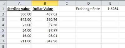
The simple formula for cell B2, would be «=A2*E1», however if you copy this down, then the formula in cell B3, would read «=A3*E2» as both references would move down a row as described above.
This is where the dollar sign ($) is used. The dollar sign allows you to fix either the row, the column or both on any cell reference, by preceding the column or row with the dollar sign. In our example if we replace the formula in cell B2 with «=A2*$E$1», then both the «E» and the «1» will remain fixed when the formula is copied. i.e. in cell B3, the formula will read «=A3*$E$1», still referring to the cell with the exchange rate in it.
In this example we have fixed both the row and the column, but in other situations, you may just want to fix one or the other, for example:

Above we have a spreadsheet calculating the times tables where we want to every cell in the white area to be the product of its row and column heading. This is easy using the dollar symbol. In cell B2, the formula without dollars would be «=A2*B1», but for this formula to work when copied to each column, we need it to always look at column A for the first reference and to work for each row, we need to always look at row 1 for the second. Using the dollar sign to do this, it becomes «=$A2*B$1». This can then be copied to every cell in the white area.
Quick Tip
You can speed up entering the dollar signs by using the function key F4 when editing the formula, if the cursor is on a cell reference in the formula, repeatedly hitting the F4 key, toggles between no dollar signs, both dollar signs, just the row and just the column.
If you enjoyed this post, go to the top of the blog, where you can subscribe for regular updates and get your free report «The 5 Excel features that you NEED to know».
The advantages of absolute references are difficult to underestimate. They often have to be used in the process of working with the program. Relative references to cells in Excel are more popular than absolute ones, but they also have their pros and cons.
In Excel, there are several types of links: absolute, relative and mixed. This also includes «names» for whole ranges of cells. Consider their possibilities and differences in practical application in formulas.
Absolute and relative links in Excel
Absolute references allow us to fix a row or column (or row and column at a time) to which the formula should refer. Relative references in Excel change automatically when you copy a formula along a range of cells, both vertically and horizontally. A simple example of relative cell addresses. Let us calculate the volume of the sphere in Excel:

- Fill the range of cells A2: A5 with different radii.
- In cell B2, enter the formula for calculating the volume of the sphere, which will refer to the value of A2. The formula will look like this: =(4/3)*3.14*A2^3
- Copy the formula from B2 along column A2: A5.
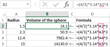
As you can see, the relative addresses help to change the address in each formula automatically.
It is also worth to point the regularity of changes in references of formulas. Data in B3 refers to A3, B4 to A4, and so on. Everything depends on where the first introduced formula will refer, and its copies will change the references relative to its position in the range of cells on the sheet.
Now instead of numbers we use absolute references:
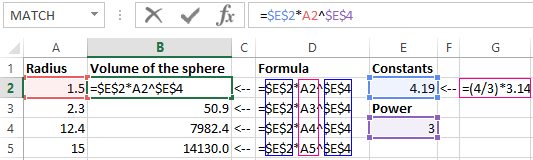
The result of the calculation is the same, but the formulas are more flexible to the changes. It is enough to change the value in one cell and the whole column is recalculated automatically. See the following example.
Use of absolute and relative links in Excel
Fill in the plate, as shown in the picture:
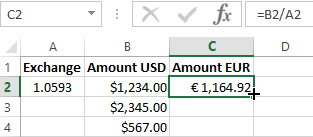
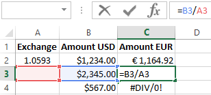
Description of the source table. In cell A2, there is an actual euro exchange rate against the dollar for today. In the range of cells B2: B4 are the amounts in dollars. In the range C2: C4 will be the amount in euros after the conversion of currencies. Tomorrow the course will change and the task of the plate will automatically recalculate the range of C2: C4 depending on the change in the value in cell A2 (that is, the euro rate).
To solve this problem, we need to enter a formula in C2: = B2 / A2 and copy it to all cells in the C2: C4 range. But here there is a problem. From the previous example, we know that when copying, relative references automatically change addresses relative to their position. Therefore, an error occurs:
Concerning the first argument, this is quite acceptable. After all, the formula automatically refers to the new value in the column of the table cells (dollar amounts). But the second indicator we need to fix on the address A2. Accordingly, it is necessary to change the relative reference to the absolute in the formula.
How to make an absolute reference in Excel? It is very simple to put the $ (dollar) symbol before the line or column number or before the both of them. Below, consider all 3 options and determine their differences.
Our new formula should contain at once 2 types of links: absolute and relative.
- In C2, enter another formula: = B2 / A $ 2. To change links in Excel, double click on the cell with the left mouse button or press the F2 key on the keyboard.
- Copy it to the other cells in the C3:C4 range.
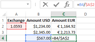
Description of the new formula. The dollar symbol ($) in the address of references fixes the address in the new copied formulas.
Absolute, relative and mixed references in Excel:
- $ A $ 2 — address of the absolute reference with fixation on columns and rows, both vertically and horizontally.
- $ A2 is a mixed link. When copying a column is fixed, and the row is changed.
- A $ 2 is a mixed link. When copying a row is fixed, and the column is changed.
For comparison: A2 is a relative address, without fixation. During the copying of the formulas, the row (2) and the column (A) automatically change to the new addresses relative to the location of the copied formula, both vertically and horizontally.
Note. In this example, the formula can contain not only a mixed link, but the absolute result: = B2 / $ A $ 2. The result will be the same. But in practice, there are often cases when you cannot do a thing without mixed references.
Helpful advice. To avoid entering the dollar symbol ($) manually, after specifying the address, press F4 repeatedly to select the required type: absolute or mixed. It’s fast and convenient.
#VALUE is Excel’s way of saying, «There’s something wrong with the way your formula is typed. Or, there’s something wrong with the cells you are referencing.» The error is very general, and it can be hard to find the exact cause of it. The information on this page shows common problems and solutions for the error.
Use the drop-down below or jump to one of the other areas:
-
Problems with subtraction
-
Problems with spaces and text
-
Other solutions to try
Fix the error for a specific function
Don’t see your function in this list? Try the other solutions listed below.

Problems with subtraction
If you’re new to Excel, you might be typing a formula for subtraction incorrectly. Here are two ways to do it:
Subtract a cell reference from another
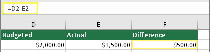
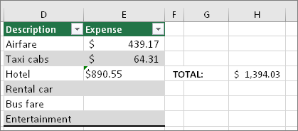
Type two values in two separate cells. In a third cell, subtract one cell reference from the other. In this example, cell D2 has the budgeted amount, and cell E2 has the actual amount. F2 has the formula =D2-E2.
Or, use SUM with positive and negative numbers
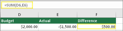
Type a positive value in one cell, and a negative value in another. In a third cell, use the SUM function to add the two cells together. In this example, cell D6 has the budgeted amount, and cell E6 has the actual amount as a negative number. F6 has the formula =SUM(D6,E6).
If you’re using Windows, you might get the #VALUE! error when doing even the most basic subtraction formula. The following might solve your problem:
-
First do a quick test. In a new workbook, type a 2 in cell A1. Type a 4 in cell B1. Then in C1 type this formula =B1-A1. If you get the #VALUE! error, go to the next step. If you don’t get the error, try other solutions on this page.
-
In Windows, open your Region control panel.
-
Windows 10: Click Start, type Region, and then click the Region control panel.
-
Windows 8: At the Start screen, type Region, click Settings, and then click Region.
-
Windows 7: Click Start and then type Region, and then click Region and language.
-
-
On the Formats tab, click Additional settings.
-
Look for the List separator. If the List separator is set to the minus sign, change it to something else. For example, a comma is a common list separator. The semicolon is also common. However, another list separator might be more appropriate for your particular region.
-
Click OK.
-
Open your workbook. If a cell contains a #VALUE! error, double-click to edit it.
-
If there are commas where there should be minus signs for subtraction, change them to minus signs.
-
Press ENTER.
-
Repeat this process for other cells that have the error.
Subtract a cell reference from another
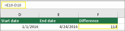
Type two dates in two separate cells. In a third cell, subtract one cell reference from the other. In this example, cell D10 has the start date, and cell E10 has the End date. F10 has the formula =E10-D10.
Or, use the DATEDIF function
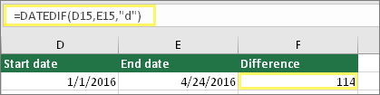
Type two dates in two separate cells. In a third cell, use the DATEDIF function to find the difference in dates. For more information on the DATEDIF function, see Calculate the difference between two dates.
Make your date column wider. If your date is aligned to the right, then it’s a date. But if it’s aligned to the left, this means the date isn’t really a date. It’s text. And Excel won’t recognize text as a date. Here are some solutions that can help this problem.
Check for leading spaces
-
Double-click a date that is being used in a subtraction formula.
-
Put your cursor at the beginning and see if you can select one or more spaces. Here’s what a selected space looks like at the beginning of a cell:

If your cell has this problem, proceed to the next step. If you don’t see one or more spaces, go to the next section on checking your computer’s date settings.
-
Select the column that contains the date by clicking its column header.
-
Click Data > Text to Columns.
-
Click Next twice.
-
On Step 3 of 3 of the wizard, under Column data format, click Date.
-
Choose a date format, and then click Finish.
-
Repeat this process for other columns to ensure they don’t contain leading spaces before dates.

Check your computer’s date settings
Excel uses your computer’s date system. If a cell’s date isn’t entered using the same date system, then Excel won’t recognize it as a true date.
For example, let’s say that your computer displays dates as mm/dd/yyyy. If you typed a date like that in a cell, Excel would recognize it as a date and you’d be able to use it in a subtraction formula. However, if you typed a date like dd/mm/yy, then Excel wouldn’t recognize that as a date. Instead, it would treat it as text.
There are two solutions to this problem: You could change the date system that your computer uses to match the date system you want to type in Excel. Or, in Excel you could create a new column and use the DATE function to create a true date based on the date stored as text. Here’s how to do that assuming your computers date system is mm/dd/yyy and your text date is 31/12/2017 in cell A1:
-
Create a formula like this: =DATE(RIGHT(A1,4),MID(A1,4,2),LEFT(A1,2))
-
The result would be 12/31/2017.
-
If you want the format to appear like dd/mm/yy, press CTRL+1 (or
+ 1 on the Mac). -
Choose a different locale that uses the dd/mm/yy format, for example, English (United Kingdom). When you’re done applying the format, the result would be 31/12/2017 and it would be a true date, not a text date.
 + 1 on the Mac).
Note: The formula above is written with the DATE, RIGHT, MID, and LEFT functions. Please notice that it is written with an assumption that the text date has two characters for days, two characters for months, and four characters for year. You may need to customize the formula to suit your date.
Problems with spaces and text
Often #VALUE! occurs because your formula refers to other cells that contain spaces, or even trickier: hidden spaces. These spaces can make a cell look blank, when in fact they are not blank.
1. Select referenced cells
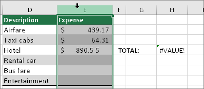
Find cells that your formula is referencing and select them. In many cases removing spaces for an entire column is a good practice because you can replace more than one space at a time. In this example, clicking the E selects the entire column.
2. Find and replace

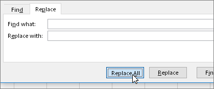
On the Home tab, click Find & Select > Replace.
3. Replace spaces with nothing
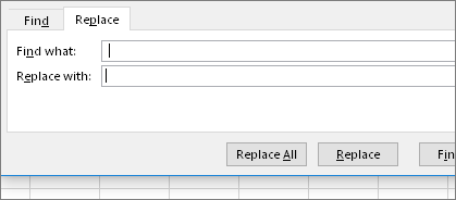
In the Find what box, type a single space. Then, in the Replace with box, delete anything that might be there.
4. Replace or Replace all
If you are confident that all spaces in the column should be removed, click Replace All. If you’d like to step through and replace spaces with nothing on an individual basis, you can click Find next first, and then click Replace when you are confident the space isn’t needed. When you’re done, the #VALUE! error may be resolved. If not, go to the next step.
5. Turn on the filter
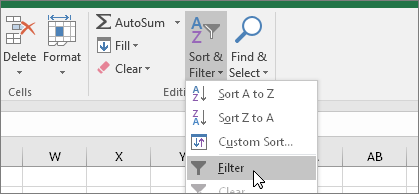
Sometimes there are hidden characters other than spaces that can make a cell appear blank, when it’s not really blank. Single apostrophes within a cell can do this. To get rid of these characters in a column, turn on the filter by going to Home > Sort & Filter > Filter.
6. Set the filter

Click the filter arrow  , and then deselect Select all. Then, select the Blanks checkbox.
7. Select any unnamed checkboxes
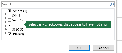
Select any check boxes that don’t have anything next to them, like this one.
8. Select blank cells, and delete

When Excel brings back the blank cells, select them. Then press the Delete key. This will clear any hidden characters in the cells.
9. Clear the filter
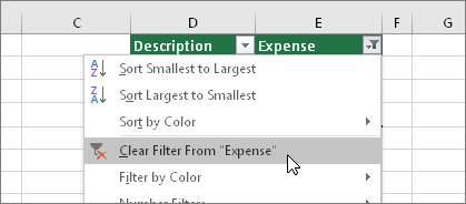
Click the filter arrow , and then click Clear filter from… so that all cells are visible.
10. Result
If spaces were the culprit of your #VALUE! error then hopefully your error has been replaced by the formula result, as shown here in our example. If not, repeat this process for other cells that your formula refers to. Or, try other solutions on this page.
Note: In this example, notice that cell E4 has a green triangle and the number is aligned to the left. This means the number is stored as text. This may cause more problems later. If you see this problem, we recommend converting numbers stored as text to numbers.
Text or special characters within a cell can cause the #VALUE! error. But sometimes it’s hard to see which cells have these problems. Solution: Use the ISTEXT function to inspect cells. Please note that ISTEXT doesn’t resolve the error, it simply finds cells that might be causing the error.
Example with #VALUE!
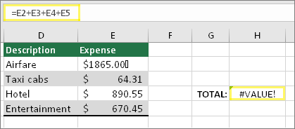
Here’s an example of a formula that has a #VALUE! error. This is likely due to cell E2. There is a special character that appears as a small box after «00.» Or as the next picture shows, you could use the ISTEXT function in a separate column to check for text.
Same example, with ISTEXT
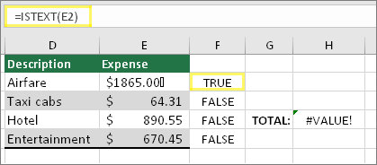
Here the ISTEXT function was added in column F. All cells are fine except the one with the value of TRUE. This means cell E2 has text. To resolve this, you could delete the cell’s contents and retype the value of 1865.00. Or you could also use the CLEAN function to clean out characters, or use the REPLACE function to replace special characters with other values.
After using CLEAN or REPLACE, you’ll want to copy the result, and use Home > Paste > Paste Special > Values. You might also have to convert numbers stored as text to numbers.
Formulas with math operations like + and * may not be able to calculate cells that contain text or spaces. In this case, try using a function instead. Functions will often ignore text values and calculate everything as numbers, eliminating the #VALUE! error. For example, instead of =A2+B2+C2, type =SUM(A2:C2). Or, instead of =A2*B2, type =PRODUCT(A2,B2).
Other solutions to try
Select the error

First select the cell with the #VALUE! error.
Click Formulas > Evaluate Formula
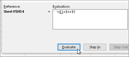
Click Formulas > Evaluate Formula > Evaluate. Excel will step through the parts of the formula individually. In this case the formula =E2+E3+E4+E5 breaks because of a hidden space in cell E2. You can’t see the space by looking at cell E2. However, you can see it here. It shows as » «.
Sometimes you just want to replace the #VALUE! error with something else like your own text, a zero or a blank cell. In this case you can add the IFERROR function to your formula. IFERROR will check to see if there’s an error, and if so, replace it with another value of your choice. If there isn’t an error, your original formula will be calculated. IFERROR will only work in Excel 2007 and later. For earlier versions you can use IF(ISERROR()).
Warning: IFERROR will hide all errors, not just the #VALUE! error. Hiding errors isn’t recommended because an error is often a sign that something needs to be fixed, not hidden. We don’t recommend using this function unless you are absolutely certain your formula works the way that you want.
Cell with #VALUE!
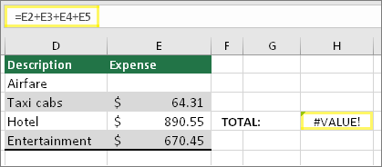
Here’s an example of a formula that has a #VALUE! error due to a hidden space in cell E2.
Error hidden by IFERROR
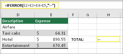
And here’s the same formula with IFERROR added to the formula. You can read the formula as: «Calculate the formula, but if there’s any kind of error, replace it with two dashes.» Note that you could also use «» to display nothing instead of two dashes. Or you could substitute your own text, such as: «Total Error».
Unfortunately, you can see that IFERROR doesn’t actually resolve the error, it simply hides it. So be certain that hiding the error is better than fixing it.
Your data connection may have become unavailable at some point. To fix this, restore the data connection, or consider importing the data if possible. If you don’t have access to the connection, ask the creator of the workbook to make a new file for you. The new file ideally would only have values, and no connections. They can do this by copying all the cells, and pasting only as values. To paste as only values, they can click Home > Paste > Paste Special > Values. This eliminates all formulas and connections, and therefore would also remove any #VALUE! errors.
See Also
Overview of formulas in Excel
How to avoid broken formulas
Below are the top 5 most common reasons why formula text is shown in cell instead of its results. They are sorted by frequency with most popular at the top.
They apply to Excel 2013 and Excel 2016.
No equal sign before the formula
Make sure that there is an equal sign before the formula.
Formula is inside quotes or apostrophes
Check that you typed formula with no quotes or apostrophes at beginning or end.
Worksheet is set to display formula – not results
Hold down theCtrl and push `
or
Click on the Formulas Tab then check if “Show Formulas” button isn’t on.

Cell is formatted as text
Sometimes showing formula as text might be due to cell format. Change it to general to see if it helps.
-
Right click on the cell with formula
-
Choose Format Cells
-
Select Category -> General
-
Click OK button


Cell with formula is locked
Found that the cell I had the formula in was “locked” (Format Cells / Protection) – it would seem that this also prevents the value from showing.
De-selecting “Locked” the value appeared immediately.
(tip from our reader Clare – thank you!)
Select cell, equal sign, type formula, enter. Now it’s one thing to write a formula that triggers an error, but to see the formula do nothing?
How do you fix something that isn’t doing anything?
It might not look so wrong but there is definitely something wrong when a formula doesn’t return a result and just… sits there.
 1")
Problem
The problem we are looking at here is a formula being entered but excel shows the formula itself instead of returning a result like so:
 2")
As you can see, there is nothing wrong with the formula (if there was, an error would show up, not the formula itself).
This happens when Excel doesn’t process the formula as a formula. Excel doesn’t evaluate it and displays the formula itself. Luckily, there aren’t too many things that could have gone wrong here so there isn’t a need to panic or delete or overwrite cells. There are a few reasons the formula shows up in place of the result and there’s an easy fix for each. Let’s dive into them.
Recommended Reading: How to Lock and Hide Formulas in Excel
Potential Issue 1 – ‘Show Formulas’ Option is Enabled
The Show Formulas feature displays all the formulas used on the sheet instead of the results of the formulas. Your sheet, which would normally look something like this:
 3")
Will look like this with Show Formulas enabled.
 4")
Widened columns with all your formulas skinned to bare the bones.
This is a favorable option for the 1-step ease of seeing all the formulas on the worksheet so you don’t have to individually select each cell and check the formula. As for the problem we are looking at right now, this option can cause confusion especially if it’s not what you need.
If it’s not what you need and you didn’t enable it yourself then how come it’s causing trouble? It may have accidentally been enabled as the keyboard shortcut for Show Formulas is Ctrl + `. It’s quite an easy mistake to make.
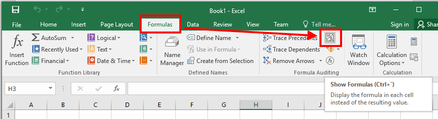
If you doubt that this is what has happened, you can check Show Formulas in the Formulas tab.
 5")
Indeed Show Formulas is enabled.
Bear in mind that this is a full worksheet feature. If all the formulas on the sheet are being displayed and that is the problem in question, the Show Formulas option needs to be addressed. If the problem is limited to one formula, Show Formulas is not your problem.
What’s the fix?
The fix is as easy as the problem itself. You can either press Ctrl + `. This is a toggle shortcut for Show Formulas and will also switch the option off.
The other way is to hit the Show Formulas button in the Formulas tab.
Both methods will disable Show Formulas.
Potential Issue 2 – Cell is Formatted as ‘Text’
The problem is the same but the reason is different. The formula is entered but the formula is displayed instead of the result. A cell in an Excel worksheet can have many formats and the default format of all cells in a new sheet is General (which would not cause this problem). Hence, a possible reason could be that the cell in which the formula is entered is formatted as Text.
 6")
What’s the fix?
The fix to this problem is to change the formatting to General. Here are the steps to do this:
- In the Home tab, in the Number section, there is a drop-down menu for cell formatting. Click the arrow to access the drop-down menu. Alternatively, right-click the cell to open the right-click context menu and select Format Cells option from the menu.
 7")
- Select General.
 8")
- Click on the formula bar (or double-click the cell) and press the Enter key.
For this case, cell formatting will be prospective. The reason for editing the formula is that formatting the cell to General will not have any impact on the cell’s existing contents.
Similarly, if you already had the result of your formula and later the cell is formatted to Text, it will not change to the formula in text. This implies that the Text format must have been applied before the formula was entered, making the formula appear as text.
Potential Issue 3 – Excel Thinks the Formula is a Text
How strange of Excel to think so but there are some very valid reasons for this. Let’s see some of them below:
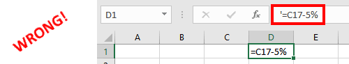
a. Apostrophe Before the Formula
You might be aware of the fact the whenever you add an apostrophe at the start in any cell, Excel considers the cell content as text. This is applicable to any data type like numbers, date-times, and even to formulas.
The apostrophe is proving to be quite a bug for us today.
 9")
While this treatment may be useful in some cases, it’s a hindrance when you’re trying to get the formula to work.
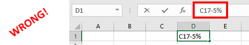
b. Equal Sign Missing or Space Before the Equal Sign
Excel recognizes and evaluates a formula when it has an equal sign in the beginning. Therefore, the lack of it will not persuade Excel to calculate it and the contents will be treated as text to be displayed as they are.
 10")
A space character before the equal sign will have a similar effect; since the first character of the formula will not be an equal sign, Excel will not evaluate it as a formula.
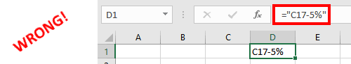
c. Formula Wrapped in Quotes
Many times while writing formulas online (on blogs or forums) people wrap them inside quotes to make them stand out. And when you try to use the same formula along with the quotes they do not work as expected.
The reason behind this is that anything that is wrapped within quotes is treated as a text by Excel and hence it does not evaluate such formulas.
 11")
Note: Please note that you are allowed to use quotes within the formulas, but using the quotes to wrap the entire formula makes excel think it is a text string and hence will not be evaluated.
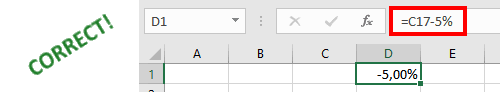
What’s the fix?
In all the above cases there is a simple fix – just edit the formula and make sure it starts with an equals sign and not with apostrophes, quotes, or unnecessary spaces.
That’s all folks! Next time you’re faced with the predicament of your formula staring at you in the face, you’ll know how to work things around it. Signing off!