
I’ve discussed on this blog before, but quite often a straight line is not the best way to represent your . For these specific situations, we can take advantage of some of the tools available to perform or in .
in with Charts
charts are a convenient way to fit a to .
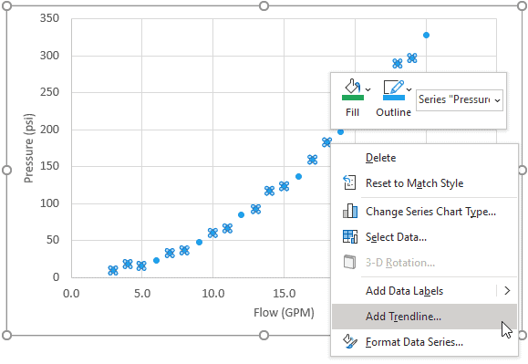
First, create a scatter .
Then right click on the series and select “Add …”
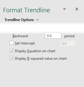
In the Format pane, select the options to on and Display R-Squared on .
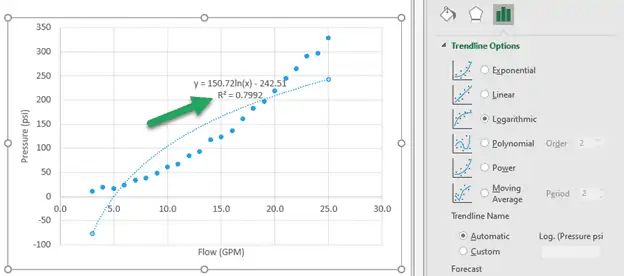
Try different types of curves to see which one maximizes the of R-squared.
For this set, a logarithmic fits the with an R-squared of 0.7992. From the image below, we can also clearly see that it is not a good fit.
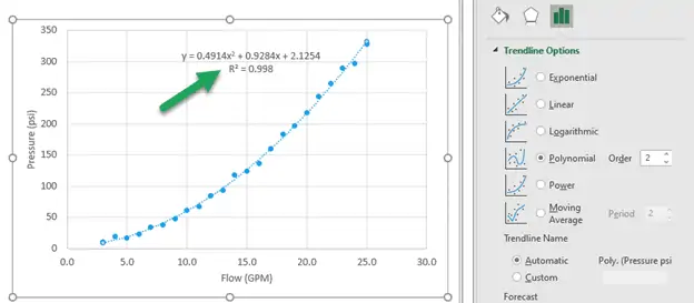
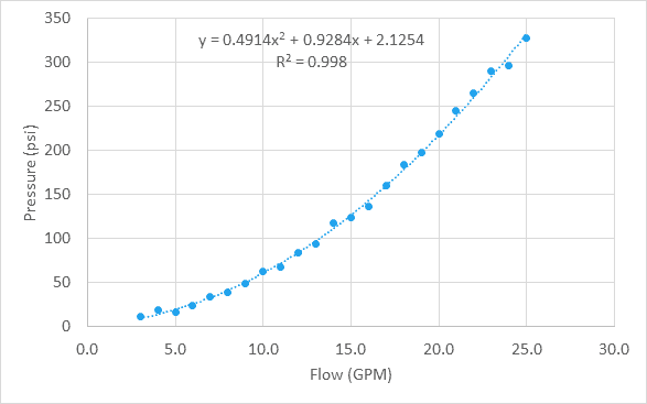
However, a second-order polynomial fits the with an R-squared of 0.998. That means the fits the better.
Although the option is convenient, it may not always be the best option when you want to know the that best fits the .
In some cases, it may provide only 1 or 2 significant digits for the . This will make any formula that uses these only accurate to the same number of significant digits.
Also, there is no way to reference the of the in the spreadsheet without manually typing them into cells. This can cause problems if the is updated, and the are not updated in the spreadsheets.
However, there is an option that provides a robust way to in using the .
Remember our old friend LINEST? Although LINEST is short for “linear estimation”, we can also use it for nonlinear with a few simple tweaks.
LINEST has the following syntax:
= LINEST(known_y’s, [known_x’s], [const], [stats])
where
- known_y’s are the y-values corresponding to the x-values which you are trying to fit (or )
- known_x’s are the known x-values (or )
- const (optional) is set to TRUE for the y-intercept to be calculated normally and set to FALSE if the y-intercept should be set to ZERO
- stats (optional) is an argument that tells whether to return . TRUE will return the statistics and FALSE will return no statistics.
Polynomial in
Let’s say we have some of pressure drop vs. flow rate through a water valve, and after plotting the on a we see that the is quadratic, as in the example above.
Even though this is nonlinear, the can also be used here to find the best fit for this . For a , we do that by using array constants .
An advantage to using LINEST to get the that define the is that we can return the directly to cells. That way we don’t have to manually transfer them out of the .
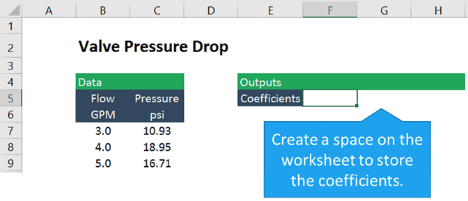
Since the is quadratic, or a second order polynomial, there are three , one for x squared, one for x, and a constant. So we’ll need to start by creating a space to store the three for the .
Using LINEST for in
The returns an array of , and optional . So we’ll need to enter it as an array formula by selecting all three of the cells for the before entering the formula.
If the cells containing the flow and pressure are named “flow” and “pressure”, the formula looks like this:
=LINEST(pressure, flow^{1,2},TRUE, FALSE)
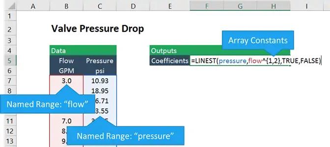
The known y’s in this case are the pressure measurements, and the known x’s are the flow measurements raised to the first and second power. The curly brackets, “{” and “}”, indicate an array constant in . Basically, we are telling to create two arrays: one of flow and another of flow-squared, and to fit the pressure to both of those arrays together.
Finally, the TRUE and FALSE arguments tell the to calculate the y-intercept normally (rather than force it to zero) and not to return additional , respectively.
Since it’s an array formula, we need to enter it by typing Ctrl+Shift+Enter .
The then returns the of x 2 and x as well as a constant (because we chose to allow LINEST to calculate the y-intercept).
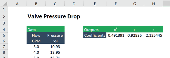
The are identical to those generated by the tool, but they are in cells now which makes them much easier to use in subsequent calculations.
For any , LINEST returns the coefficient for the highest order of the on the far left side, followed by the next highest and so on, and finally the constant.
A similar technique can be used for Exponential, Logarithmic, and Power in as well.
a Logarithmic to
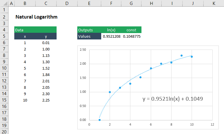
A logarithmic function has the form:
![]()
We can still use LINEST to find the coefficient, m , and constant, b , for this by inserting ln(x) as the argument for the known_x’s:
=LINEST(y_values,ln(x_values),TRUE,FALSE)
Of course, this method applies to any logarithmic , regardless of the base number. So it could be applied to an containing log10 or log2 just as easily.
in
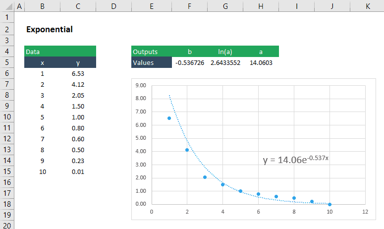
An exponential function has the form:
![]()
It’s a little trickier to get the a and b for this because first we need to do a little algebra to make the take on a “linear” form. First, take the natural log of both sides of the to get the following:
![]()
Now we can use LINEST to get ln(a) and b by entering ln(y) as the argument for the y_values:
=LINEST(ln(y_values),x_values,TRUE,FALSE)
The second returned by this array formula is ln(a), so to get just “a” , we would simply use the exponential :
![]()
Which, in an , translates to:
=EXP(number)
a Power to
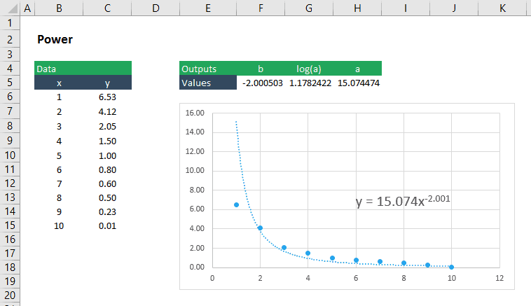
A power can be fit to using LINEST in much the same way that we do it for an exponential . A power has the form:
![]()
Again, we can “linearize” it by taking the base 10 log of both sides of the to obtain:
![]()
With the in this form, the to return b and log 10 (a) can be set up like this:
=LINEST(LOG10(yvalues),LOG10(xvalues),TRUE,FALSE)
Since the returns b and log10(a) , we’ll have to find a with the following formula:
![]()
In , that formula is:
=10^(number)
That’s it for now. As you can see, there are a number of ways to use the for nonlinear in .
A straight line is not always the best method to fit your data points. For these specific cases, we can use some of the tools available in Excel to do nonlinear regression or curve fitting.
Without any further ado, let’s get started with performing curve fitting in Excel today. We’ll explore the different methods to do so now.
1. Polynomial Curve Fitting Model
Let’s consider some data points in x and y, we find that the data is quadratic after plotting it on a chart. A polynomial function has the form: y = ax2+ bx + c

Although this data is nonlinear, the LINEST function can be utilized to obtain the best fit curve. We can return the coefficients straight to cells when we use LINEST to acquire the coefficients that define the polynomial equation.
There are three coefficients, a for x squared, b for x, and a constant c since the equation is quadratic, or a second-order polynomial. Follow these steps to obtain the coefficients a, b and c:
- Select the cell where you want to calculate and display the coefficients.
- Type the formula =LINEST(y, x^{1,2}, TRUE, FALSE), where y is the cells containing the known y data and x is the cells containing the known x data raised to the first and second power. Finally, the TRUE and FALSE parameters instruct the LINEST function to calculate the y-intercept without forcing it to zero and not to return further regression data, respectively.

- Press the Ctrl+Shift+Enter keys to return the result.

Therefore, the polynomial curve fitting formula for the given dataset is: y = 1.07x2+ 0.01x + 0.04
2. Logarithmic Curve Fitting Model
Let’s consider some data points in x and y, we find that the data is logarithmic after plotting it on a chart. A logarithmic function has the form: y = m.ln(x) + b

Although this data is nonlinear, the LINEST function can be utilized to obtain the best fit curve. We can return the coefficients straight to cells when we use LINEST to acquire the coefficients that define the logarithmic equation.
There are two coefficients, m for ln(x) and a constant b. Follow these steps to obtain the coefficients m and b:
- Select the cell where you want to calculate and display the coefficients.
- Type the formula =LINEST(y, LN(x), TRUE, FALSE), where y is the cells containing the known y data and x is the cells containing the known x data. Finally, the TRUE and FALSE parameters instruct the LINEST function to calculate the y-intercept without forcing it to zero and not to return further regression data, respectively.

- Press the Ctrl+Shift+Enter keys to return the result.

Therefore, the logarithmic curve fitting formula for the given dataset is: y = 0.91ln(x) + 0.18
3. Exponential Curve Fitting Model
Let’s consider some data points in x and y, we find that the data is exponential after plotting it on a chart. A logarithmic function has the form: y = aebx

It’s a little more difficult to find the coefficients, a and b, for this equation since we need to do some algebra first to make the equation take on a “linear” form. To begin, compute the natural log of both sides of the equation to obtain the following: ln(y) = ln(a) + bx.
We can now use LINEST to get ln(a) and b by entering ln(y) as the y values argument using the formula =LINEST(LN(y), x, TRUE, FALSE). From ln(a), we can simply apply the exponential function to get just “a” as a = eln(a) . Follow these steps to obtain the coefficients a and b:
- Select the cell where you want to calculate and display the coefficients.
- Type the formula =LINEST(LN(y), x, TRUE, FALSE), where y is the cells containing the known y data and x is the cells containing the known x data. Finally, the TRUE and FALSE parameters instruct the LINEST function to calculate the y-intercept without forcing it to zero and not to return further regression data, respectively.

- Press the Ctrl+Shift+Enter keys to return the result for b and ln(a).

- To get the value of a, type =EXP(F2), where cell F2 contains the value of ln(a).

- Press the Enter key to display the result.

Therefore, the exponential curve fitting formula for the given dataset is: y = 8.61e-0.38x
4. Power Curve Fitting Model
Let’s consider some data points in x and y, we find that the data is in power model form after plotting it on a chart. A power function has the form: y = axb

It’s a little more difficult to find the coefficients, a and b, for this equation since we need to do some algebra first to make the equation take on a “linear” form. To begin, compute the natural log of both sides of the equation to obtain the following: ln(y) = ln(a) + bln(x). We can now use LINEST to get ln(a) and b by entering ln(y) as the y values argument and ln(x) as the x values argument using the formula =LINEST(LN(y), LN(x), TRUE, FALSE). From ln(a), we can simply apply the exponential function to get just “a” as a = eln(a). Follow these steps to obtain the coefficients a and b:
- Select the cell where you want to calculate and display the coefficients.
- Type the formula =LINEST(LN(y), LN(x), TRUE, FALSE), where y is the cells containing the known y data and x is the cells containing the known x data. Finally, the TRUE and FALSE parameters instruct the LINEST function to calculate the y-intercept without forcing it to zero and not to return further regression data, respectively.

- Press the Ctrl+Shift+Enter keys to return the result for b and ln(a).

- To get the value of a, type =EXP(F2), where cell F2 contains the value of ln(a).

- Press the Enter key to display the result.

Therefore, the power function curve fitting formula for the given dataset is: y = 11.33x-1.56
Conclusion
In this tutorial, we learned how to perform curve fitting In Excel using different models.
References
- LINEST function (microsoft.com)
Often you may want to find the equation that best fits some curve for a dataset in Excel.

Fortunately this is fairly easy to do using the Trendline function in Excel.
This tutorial provides a step-by-step example of how to fit an equation to a curve in Excel.
Step 1: Create the Data
First, let’s create a fake dataset to work with:

Step 2: Create a Scatterplot
Next, let’s create a scatterplot to visualize the dataset.
First, highlight cells A2:B16 as follows:

Next, click the Insert tab along the top ribbon, and then click the first plot option under Scatter:

This produces the following scatterplot:

Step 3: Add a Trendline
Next, click anywhere on the scatterplot. Then click the + sign in the top right corner. In the dropdown menu, click the arrow next to Trendline and then click More Options:

In the window that appears to the right, click the button next to Polynomial. Then check the boxes next to Display Equation on chart and Display R-squared value on chart.

This produces the following curve on the scatterplot:

The equation of the curve is as follows:
y = 0.3302x2 – 3.6682x + 21.653
The R-squared tells us the percentage of the variation in the response variable that can be explained by the predictor variables. The R-squared for this particular curve is 0.5874.
Step 4: Choose the Best Trendline
We can also increase the order of the Polynomial that we use to see if a more flexible curve does a better job of fitting the dataset.
For example, we could choose to set the Polynomial Order to be 4:

This results in the following curve:

The equation of the curve is as follows:
y = -0.0192x4 + 0.7081x3 – 8.3649x2 + 35.823x – 26.516
The R-squared for this particular curve is 0.9707.
This R-squared is considerably higher than that of the previous curve, which indicates that it fits the dataset much more closely.
We can also use this equation of the curve to predict the value of the response variable based on the predictor variable. For example if x = 4 then we would predict that y = 23.34:
y = -0.0192(4)4 + 0.7081(4)3 – 8.3649(4)2 + 35.823(4) – 26.516 = 23.34
You can find more Excel tutorials on this page.
When we have a set of data and we want to determine the relationship between the variables through regression analysis, we can create a curve that best fits our data points. Fortunately, Excel allows us to fit a curve and come up with an equation that represents the best fit curve.
 Figure 1. Final result: Curve fitting
How to fit a curve
In order to fit a curve to our data, we follow these steps:
- Select the data for our graph, B2:C17, which is a tabular result of the relationship between temperature and volume.
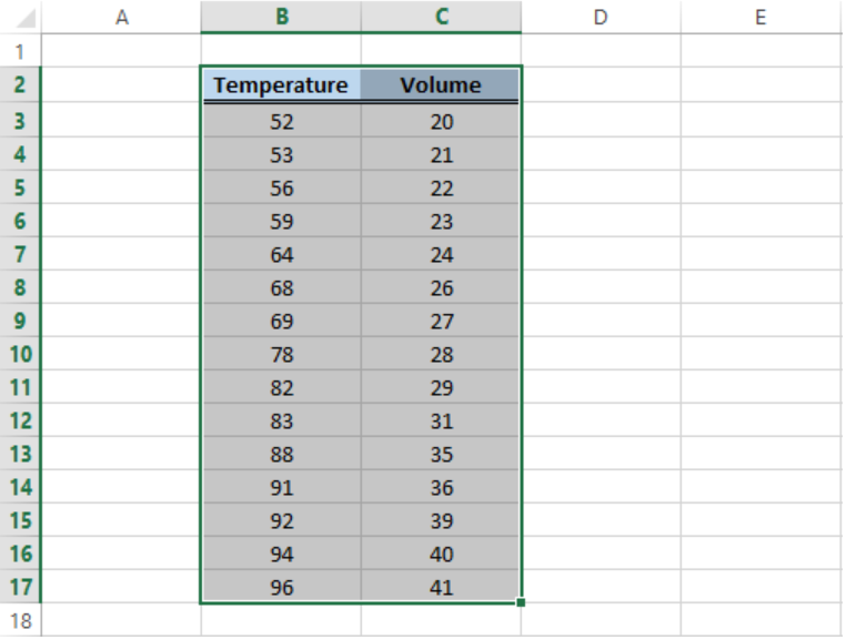 Figure 2. Sample data for curve fitting
- Click Insert tab > Scatter button > Scatter chart
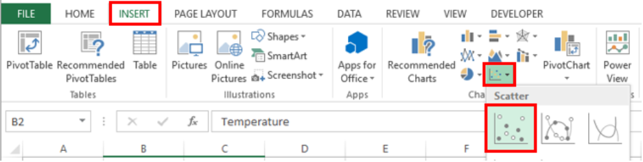 Figure 3. Scatter chart option
- A Scatter plot will be created, and the Design tab will appear in the toolbar under Chart Tools.
- Click Add Chart Element > Trendline > More Trendline Options
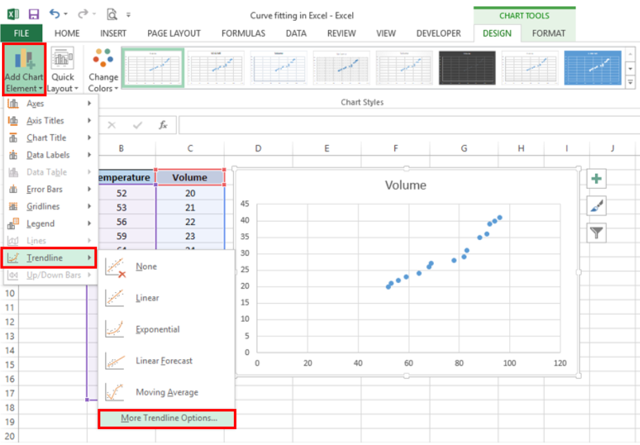 Figure 4. Add Trendline options
- In the Format Trendline window, select Polynomial and set the Order to “2”
- Check the option for “Display Equation on chart”.
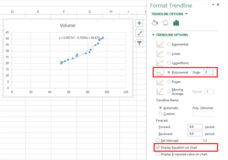 Figure 5. Format Trendline dialog box
Excel will instantly add the best fit curve for our data, and display the polynomial equation on the chart. We can add the R-squared value as a measure of how close our data points are to the regression line. We simply have to check the option for “Display R-squared value on chart”.
In curve fitting, we want the R-squared value to be as close to the value of 1 as possible. The image below shows our scatter plot with a polynomial trendline to the order of 2. The R-squared value is “0.9759”.
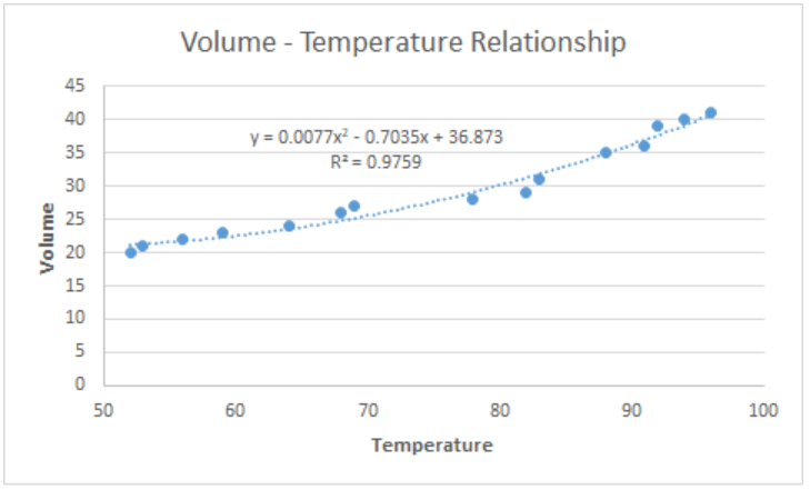 Figure 6. Output: How to fit a curve
Customize the best fit curve
We can further customize our chart by adding axis titles, adjusting the minimum axis values and highlighting the best fit curve by changing the color.
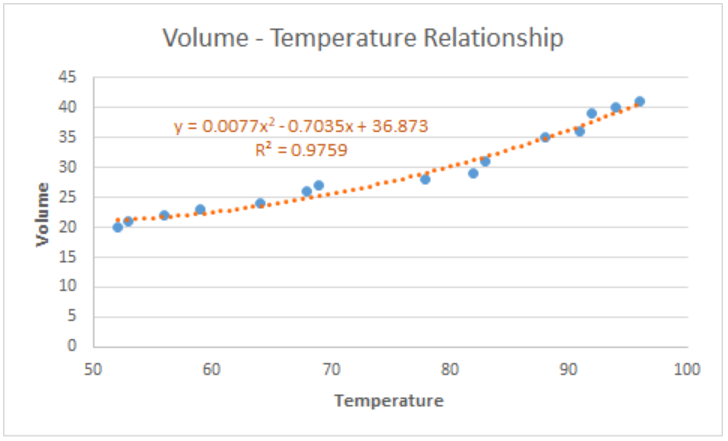 Figure 7. Output: Customize best fit curve
Note:
We can opt to add a linear trendline instead, but a linear curve fit is not the best fit for our data. As shown below, several data points fall far from the linear trendline.
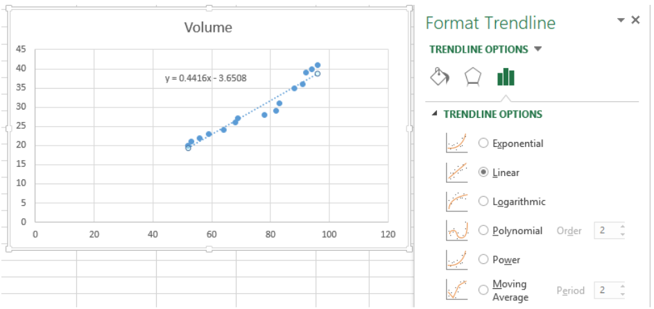 Figure 8. Linear curve fit
Instant Connection to an Excel Expert
Most of the time, the problem you will need to solve will be more complex than a simple application of a formula or function. If you want to save hours of research and frustration, try our live Excelchat service! Our Excel Experts are available 24/7 to answer any Excel question you may have. We guarantee a connection within 30 seconds and a customized solution within 20 minutes.
Contents
- 1 How do you make a curve fitting?
- 2 How do you switch axis on Excel?
- 3 How do I plot a graph in Excel?
- 4 What is a curve fitting computer simulation program?
- 5 What is SSE in curve fitting?
- 6 What is the command used for opening curve fitting?
- 7 How do I change the axis scale in Excel 2020?
- 8 How do you join two graphs together?
- 9 How do I combine two bar charts in Excel?
- 10 Can you do a graph in Excel?
- 11 What is Pivot in Excel?
- 12 How do you plot XY points in Excel?
- 13 Why do we use curve fitting?
- 14 How do you calculate SST and SSR?
- 15 What is SSR in stats?
- 16 Is r-squared goodness of fit?
- 17 What is SSE Matlab?
- 18 How do I save a Curve Fitting in Matlab?
- 19 How do I smooth a curve in Matlab?
How do you make a curve fitting?
The most common way to fit curves to the data using linear regression is to include polynomial terms, such as squared or cubed predictors. Typically, you choose the model order by the number of bends you need in your line. Each increase in the exponent produces one more bend in the curved fitted line.
How do you switch axis on Excel?
How to switch axes in excel
- Click on the chart and choose the Design tab,
- Go to Data >> Switch Row / Column.
- Now, the X-axis switched with the Y-axis without the need for transposing data.
How do I plot a graph in Excel?
How to Make a Chart in Excel
- Step 1: Select Chart Type. Once your data is highlighted in the Workbook, click the Insert tab on the top banner.
- Step 2: Create Your Chart.
- Step 3: Add Chart Elements.
- Step 4: Adjust Quick Layout.
- Step 5: Change Colors.
- Step 6: Change Style.
- Step 7: Switch Row/Column.
- Step 8: Select Data.
What is a curve fitting computer simulation program?
Curve fitting is one of the most powerful and most widely used analysis tools in Origin. Curve fitting examines the relationship between one or more predictors (independent variables) and a response variable (dependent variable), with the goal of defining a “best fit” model of the relationship.
What is SSE in curve fitting?
Sum of Squares Due to Error.
This statistic measures the total deviation of the response values from the fit to the response values. It is also called the summed square of residuals and is usually labeled as SSE. A value closer to 0 indicates a better fit.
What is the command used for opening curve fitting?
Load data at the MATLAB and in command line type pwd. Open the Editor and type the code for curve fit. Write a different equation to select Polynomial. Also, we can fit by using a curve fit toolbox.
How do I change the axis scale in Excel 2020?
Changing the Axis Scale
- Right-click on the axis whose scale you want to change. Excel displays a Context menu for the axis.
- Choose Format Axis from the Context menu.
- Make sure Axis Options is clicked at the left of the dialog box.
- Adjust the scale settings (top of the dialog box—Minimum, Maximum, etc.)
- Click on OK.
How do you join two graphs together?
Merge Multiple Graphs
- Click on the Rescale button when the Graph 1 in the Arranging Layers subfolder is active.
- Select Graph: Merge Graph Windows in the main menu to open the dialog.
- Do the following:
- Click OK to close the dialog box.
How do I combine two bar charts in Excel?
Highlight the second set of data, making sure to unhighlight the first set of data. Press “Ctrl+c” to copy the information. Click on the graph and press “Ctrl+v.” This should insert the second set of information into the graph. Repeat for any other pieces of information.
Can you do a graph in Excel?
How to Make a Graph in Excel
- Enter your data into Excel.
- Choose one of nine graph and chart options to make.
- Highlight your data and click ‘Insert’ your desired graph.
- Switch the data on each axis, if necessary.
- Adjust your data’s layout and colors.
- Change the size of your chart’s legend and axis labels.
What is Pivot in Excel?
A pivot table in Excel is an extraction or resumé of your original table with source data. A pivot table can provide quick answers to questions about your table that can otherwise only be answered by complicated formulas.
How do you plot XY points in Excel?
Go to the “Insert” tab and look for the “Charts” section. In Excel 2007 and earlier versions, click on “Scatter” and choose one of the options that appear in the drop-down menu. In Excel 2010 and later, look for the icon with dots plotted in the xy plane that says “Insert Scatter (X, Y) or Bubble Chart.”
Why do we use curve fitting?
Fitted curves can be used as an aid for data visualization, to infer values of a function where no data are available, and to summarize the relationships among two or more variables.
How do you calculate SST and SSR?
SST = SSR + SSE.
We can also manually calculate the R-squared of the regression model:
- R-squared = SSR / SST.
- R-squared = 917.4751 / 1248.55.
- R-squared = 0.7348.
What is SSR in stats?
In statistics, the residual sum of squares (RSS), also known as the sum of squared residuals (SSR) or the sum of squared estimate of errors (SSE), is the sum of the squares of residuals (deviations predicted from actual empirical values of data).
Is r-squared goodness of fit?
R-squared is a goodness-of-fit measure for linear regression models.R-squared measures the strength of the relationship between your model and the dependent variable on a convenient 0 – 100% scale. After fitting a linear regression model, you need to determine how well the model fits the data.
What is SSE Matlab?
sse is a network performance function. It measures performance according to the sum of squared errors. perf = sse( net , t , y , ew , Name,Value ) has two optional function parameters that set the regularization of the errors and the normalizations of the outputs and targets. sse is a network performance function.
How do I save a Curve Fitting in Matlab?
To export a fit to the MATLAB workspace, follow these steps: Select a fit and save it to the MATLAB workspace using one of these methods: Right-click the fit listed in the Table of Fits and select Save myfitname to Workspace. Select a fit figure in the Curve Fitting app and select Fit > Save to Workspace.
How do I smooth a curve in Matlab?
Fit smoothing splines in Curve Fitting app or with the fit function to create a smooth curve through data and specify the smoothness. Fit smooth surfaces to your data in Curve Fitting app or with the fit function using Lowess models.