Fit pages in excel

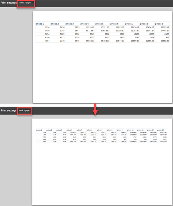
By scaling your worksheet for printing, you can make your data fit to one page. You can shrink your Excel document to fit data on a designated number of pages using the Page Setup option in the Page Layout tab.

Shrink a worksheet to fit on one page

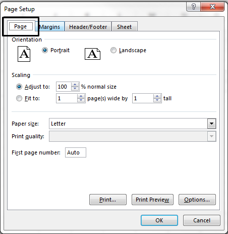
1. Click Page Layout. Click the small Dialog Box Launcher on the bottom right. This opens up the Page Setup dialog box.

   

2. Select the Page tab in the Page Setup dialog box.

   

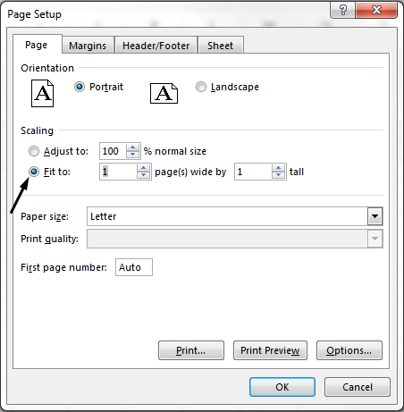
3. Select Fit to under Scaling.

4. To fit your document to print on one page, choose 1 page(s) wide by 1 tall in the Fit to boxes.

   

   Note: Excel will shrink your data to fit on the number of pages specified. You can also adjust the Fit to numbers to print to multiple pages.

5. Press OK at the bottom of the Page Setup dialog box.

See Also

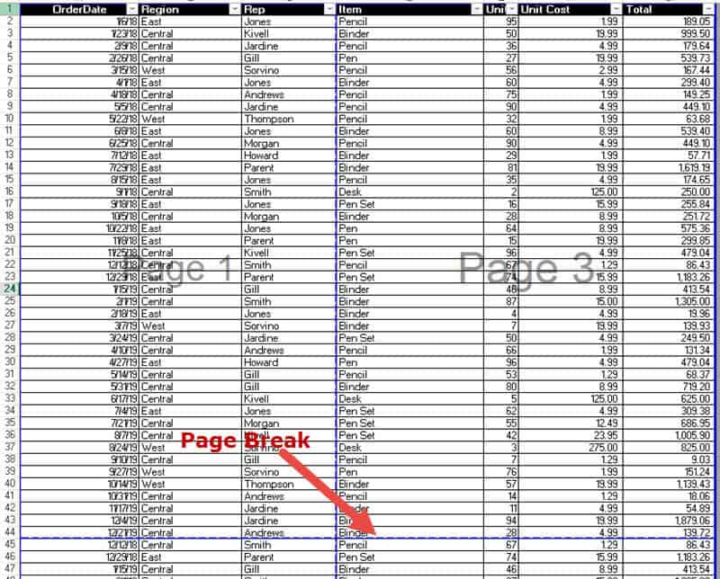
You can also use page breaks to divide your worksheet into separate pages for printing. While Excel does add page breaks automatically (indicated by a dashed line), you can also insert, move, or delete page breaks in a worksheet.

If you only need to print a section of your worksheet, you can set or clear a print area on a worksheet.

This feature is not available in Excel for the web.

If you have the Excel desktop application, you can use the Open in Excel button to open the workbook and scale the worksheet to fit data on one page.

Picture this – you’ve worked hard to get your spreadsheet to look just right.

You’ve sized the columns correctly, you’ve put nice colored headings, and everything looks great on the screen.

And now when you hit that Print button, it doesn’t work as you expected!

Your last 2 columns are appearing on the second page and you’re not sure where most of your rows have gone!

Unlike Microsoft Word, printing Excel worksheets is surprisingly not as intuitive as you would think.

This is because your spreadsheets are not always sized the same.

So it’s no surprise if you find your columns splitting in the most awkward places or if you find few rows on one page and few on the others.

You might also find it difficult to control the size of the text in your printout.

Fortunately, there are ways around this.

In this tutorial, you’ll see two ways to fit your Excel data (rows and columns) into one page.

I will also point out certain issues you are likely to face while printing and how to solve them.

Method 1: Fitting data to Page in Excel using Page Setup

Below are the steps to scale the data in the worksheet to fit on one page:

1. From the Page Layout tab, you will find the ‘Scale to Fit’ group. This lets you adjust the width and height of your printout to fit a certain number of pages.
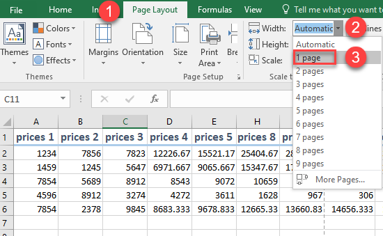
2. If you want your whole worksheet to be printed on exactly one sheet of paper, set Width and Height both to “1 page” by selecting it from the dropdown menu.
3. Check how your printout is going to look by navigating to File->Print. If everything went right, you should see all your data fit into a single page.

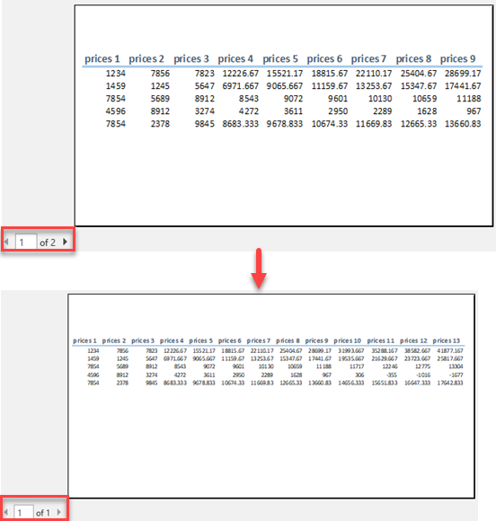
When you use this option to scale the page and fit data on one page, it will make the data look small (as Excel tries to squeeze more data in the same space. This works fine if you only have a few extra rows or columns, but if you have a lot, fitting all of it in one page may not be a good idea.

Method 2: Fitting data to Page in Excel using Print Preview Screen

You can also scale the data to fit on one page while you’re printing the data.

This does exactly the same thing that I did in the previous method (just the option to do it is in a different place).

Below are the steps to fit data on one page while printing:

1. Click the File tab
2. Click on the Print option. This will open the Print Preview screen.
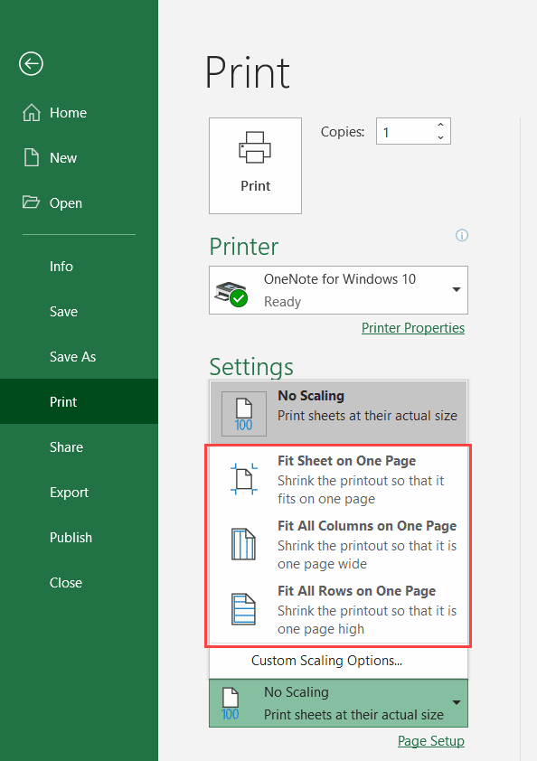
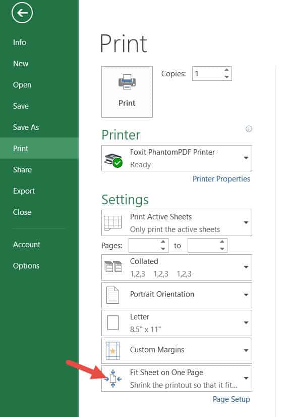
3. On the left-hand side of the screen, you will see a ‘Settings’ section. The last option under this section is most likely a dropdown that says “No Scaling”. Select the arrow for this dropdown.
4. Select “Fit Sheet on One Page”
5. Check if you got everything on a single page from the preview on the right-hand side of the screen. If everything looks fine, you can go ahead and hit the Print button.

Autofit only the Width or Height into a Single Page

If you have too much data in too many columns, your printout might turn out too tiny and look illegible. There are ways around this.

• If you need all your columns within 1 page, but don’t mind splitting the rows to 2, 3, or how many ever pages needed, then leave the Height option blank if using the first method. If using the second method, select “Fit all Columns on One Page” instead of “Fit Sheet on One Page”.
• Similarly, if you want all your rows to fit in a single page and don’t mind columns spanning separate pages, then leave the Width option blank if using the first method. If using the second method, select “Fit all Rows on One Page”.

Another option is to use page breaks to divide your worksheet.

Using Page Breaks to divide your Worksheet’s Print Areas

Page Breaks are dividers that specify the areas where your sheet will break into separate pages when printed.

Excel automatically adds page breaks, unless you specify them yourself.

It fixes these page breaks depending on your page size, margins, and scale options to ensure that an optimal number of columns and rows appear on each page.

1. To see the page breaks, (indicated by a dashed line), select ‘Page Break View’ from the View tab (Under the ‘Workbook Views’ group).
2. You will see the page break demarcations in the form of blue dashed lines. You can now move these dashed lines to accommodate the number of rows and columns you need to fit in one page.
3. To return to Normal view, just select ‘Normal’ from the View Tab. Make sure to preview the pages before printing.

If you have selected the ‘Fit Sheet on One Page’ from the Print Settings area, you will not be able to set the page breaks (as Excel already knows it needs to fit all the data in one sheet). If you want to set the page breaks, then you need to go the Print settings (click on File >> Print >> Settings) and select ‘No Scaling’ from the last dropdown

Points to Remember when Printing your Worksheet

• Excel lets you select a portion of your worksheet that you want to solely print on a single page. For this, select the area that you want to print on one page. Then, select Print Area from the Page Layout tab, under the ‘Page Setup’ group. From the dropdown menu that appears, select ‘Set Print Area’. If you see the print preview now, you will see only your selected area ready to print on your page. To clear your selected print area, just select ‘Clear Print Area’.
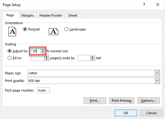
• If you find your selected area is too small or too large for the page, you can shrink or enlarge it as needed. For this, select the Dialog box launcher ( ) from the ‘Scale to Fit’ group under the Page Layout tab. This will open the Page Setup dialog box. Under the ‘Scaling’ section, select the radio button next to ‘Adjust to’ and set percentage to the size you want. If you want to enlarge your selected area to fit the page, then select a number more than 100%. If you want to shrink it to fit the page, then select a number less than 100%.
• If your sheet has quite a lot of columns, it may be wiser to change the page orientation and print your sheet in Landscape mode, rather than Portrait. For this, navigate to the Page Setup dialog box and select the radio button next to the Landscape option (under the Orientation section).
• The default paper size setting is usually ‘Letter (8.5” x 11”)’. If you are using a different sized paper, you can change the paper size settings from the Page Setup dialog box. Under the Scaling section, next to ‘Paper size’, click on the dropdown arrow and select the appropriate paper size from the list.

In this tutorial, I showed you two ways to fit your worksheet into one page.

We have also provided some tips to not just fit your sheet to a page, but to do so in such a way that your printout is legible and looks elegant. I hope you found this tutorial helpful.

Other Excel tutorials you may find useful:

• How to Print Multiple Tabs/Sheets in Excel
• How to Set a Row to Print on Every Page in Excel
• How to Center the Worksheet Horizontally on the Page in Excel
• How to Make all Cells the Same Size in Excel (AutoFit Rows/Columns)
• How to Print Row Numbers in Excel
• How to Print Gridlines in Excel
• How to Remove Page Breaks in Excel?

Shrink a worksheet to fit on one page Select the Page tab in the Page Setup dialog box. Select Fit to under Scaling. To fit your document to print on one page, choose 1 page(s) wide by 1 tall in the Fit to boxes. Note: Excel will shrink your data to fit on the number of pages specified.

How do I get my Excel spreadsheet to print on one page?

Print a sheet on one page
On the Page Layout tab, select Page Setup. Under Scaling, select Fit to, and type 1 in both the page(s) wide box and page(s) tall box. Select OK. On the File menu, select Print.

How do I get Excel to only show one page?

Select the range you want to view on a single screen. Select the View tab on Excel’s ribbon.
As shown in Figure 5, you can choose from these additional options:

1. Fit All Rows on One Page. Select this option if your data spans many rows.
2. Fit All Columns on One Page.
3. Fit Sheet on One Page.

Where is the page layout in Excel?

Locate and select the Page Layout view command at the bottom of the Excel window. The worksheet will appear in Page Layout view.

How do I make columns fit on one page in Excel?

Follow these steps: Click the Page Layout tab on the ribbon. In the Scale to Fit group, in the Width box, select 1 page, and in the Height box, select Automatic. Columns will now appear on one page, but the rows may extend to more than one page.

How do I make my Excel sheet A4 size?

Step 1: Open your file in Excel 2013. Step 2: Click the Page Layout tab at the top of the window. Step 3: Click the Size button in the Page Setup section of the ribbon, then click the A4 option.

How do I make the grids show up when I print in Excel?

How to Show Grid Lines When Printing in Microsoft Excel

1. Select the worksheet or worksheets you want to print, and then click the “Page Layout” tab.
2. Check “Print” under Gridlines in the Sheet Options group, and then press “Ctrl-P” to go to the Print window.

How do I reduce the screen size in Excel?

How do I reduce to screen size of excel?

1. Go to control panel.
2. Select all control panel items.
3. Click on display.
4. Under change only the text size, click the dropdown and select menus.
5. From the dropdown, select the size of your choice.

How can I reduce my Excel file size?

Ways to Reduce Excel File Size

1. Remove unnecessary worksheets, data, and formulas. The number of worksheets and the amount of data contained in an Excel file are directly related to the size of the file.
2. Remove formatting.
3. Remove Pivot Cache.
4. Save in binary format (.
5. Compress the file.

How do I get Excel to show all pages?

First ensure that the Show sheet tabs is enabled. To do this, For all other Excel versions, click File > Options > Advanced—in under Display options for this workbook—and then ensure that there is a check in the Show sheet tabs box.

Why does my excel not have Page Layout?

If it’s checked and can’t see the Page Layout tab, please follow the below steps: Open the Excel application> File> Options> Customize Ribbon> Under Choose commands from, selects All Tabs> Select Page Layout> Click Add> OK.

How do I fix the Page Layout in Excel?

Press CTRL and then click each worksheet tab in the workbook that you want to affect. On the File menu, click Page Setup. In Excel 2007, click the dialog box launcher in the Page Setup group in the Page Layout tab. Make the changes that you want in the Page Setup dialog box, and then click OK.

How do I make all Excel tabs the same size?

To zoom all or some tabs in one size of a workbook, you can select the sheet tabs first, and then zoom them. Select first tab and the hold Shift key to select the last tab in the Sheet tab bar, then drag zoom slider to change the their zoom levels.

How do I fix scaling issues in Excel?

Select Display > Change the size of text, apps, and other items, and then adjust the slider for each monitor. Right-click the application, select Properties, select the Compatibility tab, and then select the Disable display scaling on high DPI settings check box.

How do I apply a preset margin option?

Use the File menu:

1. From the File menu, select Print.
2. Under “Settings”, select the Normal Margins drop-down menu.
3. Choose a different pre-set option, or select Custom Margins…, adjust the values for each margin that you want to change, and click OK.

How will you apply your own border style on a cell?

Advanced Border Options

1. Select the cell(s) where you want to add the border.
2. Click the Font dialog box launcher.
3. Click the Border tab.
4. Select the line style and color you want.
5. Select a preset option or apply borders individually in the Borders section.
6. Click OK.

How do I set paper size in Excel Windows 10?

Add Custom Paper Size in Windows 10
In the dialog box that appears, click “Printing Preferences”. On the “Paper/Quality” tab, under “Print Quality”, select “Custom Options”. Under “Paper Options”, select “Custom” and enter the appropriate width and height. Be sure to set your width smaller than your length.

How do you fit an Excel table in Word?

To adjust table row and column size in Word:

1. To fit the columns to the text (or page margins if cells are empty), click [AutoFit] > select “AutoFit Contents.”
2. To fit the table to the text, click [AutoFit] > select “AutoFit Window.”

Why are gridlines not showing in Excel?

Click on the View tab, then check the box for Gridlines in the Show group. If the background color for a cell is white instead of no fill, then it will appear that the gridlines are missing. Select the cells that are missing the gridlines, or hit Control + A to select the entire worksheet.

Why is my Excel spreadsheet not printing gridlines?

If gridlines don’t appear in the print preview or the resulting printout, you probably have the “Draft quality” enabled for your printer. This mode is designed to save ink, so it omits things like the gridlines. To disable this option, click File > Print > Page Setup in Excel. Click the “Sheet” tab.

Why are some of my borders not showing in Excel when printing?

If you are using Microsoft Excel 2010+ (i.e. a version later than Office 2010), Navigate to the Layout tab. There are 4 sub-sections there namely: Page Setup, View, Print and Window. Under the Print sub-section, check the Gridlines option. That should do it.

See all How-To Articles

This tutorial demonstrates how to scale your print area to fit a page in Excel and Google Sheets.

Scale to Fit Page

To achieve a better fit on printed pages you can shrink or enlarge a worksheet.

1. In the Ribbon, go to Page Layout and click the arrow in the lower-right corner of the Scale to Fit group.

1. This opens the Page Setup dialog box. In the Adjust to box, enter the percent to scale to and click OK. Here, 50% means that the worksheet would print at half its normal size.

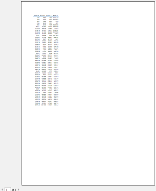
As a result, the worksheet is reduced or enlarged according to the percentage you entered.

Note: To reduce a worksheet, enter a number that is smaller than 100%; to enlarge a worksheet, enter a number greater than 100%.

Scale to Fit Height

If you have a lot of rows in the worksheet, you can use Scale to Fit to reduce the size of it in order to better fit the printed page.

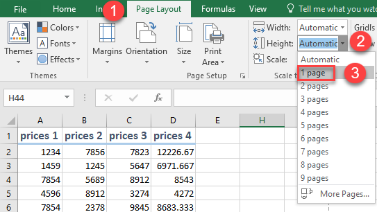
1. In the Ribbon, go to Page Layout.
2. In the Scale to Fit group, click the arrow next to Height.
3. Choose the number of pages (here, 1 page).

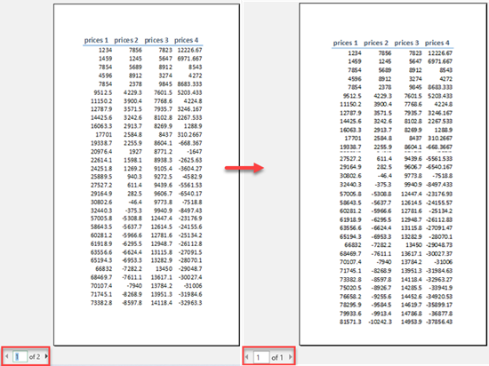
As a result, all rows are printed on one page. (But keep in mind that columns may extend to more than one page.)

Note: The printout may be difficult to read because of the data shrinkage, so you should check how much scaling has been done by looking at the number in the Scale box. If the number is low, you may need to adjust the layout or change the page’s orientation.

Scale to Fit Width

If you have a lot of columns in the worksheet, you can use Scale to Fit to reduce the size of it in order to better fit the printed page.

1. In the Ribbon, go to Page Layout > Scale to Fit.
2. Click on the arrow next to Width.
3. Choose the number of pages (here, 1 page).

As a result, all columns are printed on one page.

Scale to Fit in Google Sheets

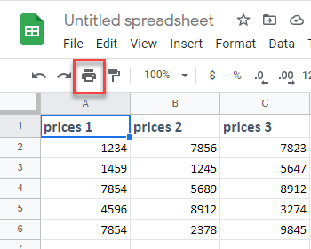
1. To scale worksheet in Google Sheets, in the Toolbar, click the Print icon (or press CTRL + P).

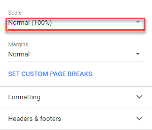
1. This opens the Print settings menu. Under Scale, click the arrow to the right of the box to display preset scale options.

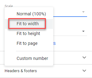
1. Choose a scaling option (here, Fit to width).

As a result, the columns are scaled to fit one page.

If you often print your data/work in Excel, I am sure you have faced the issue where it prints multiple pages instead of one single page.

Sometimes, it’s so frustrating that a new page is printed just to accommodate a few extra lines of data (which also leads to wastage of paper).

There are some simple techniques you can use to make sure you Excel data in printed on one page (or in less number of pages in case you’re printing a big report).

In this Excel tutorial, I will share some methods you can use to print the Excel sheet on one page. You can use a combination of these methods to get the best result.

So let’s get started!

Check How Many Pages Would be Printed (Preview)

Before you set out to optimize the settings to print the Excel work in one sheet, it’s best to check the current state using the Print Preview.

Don’t worry! You don’t have to print anything for this. You can simply check how the printed work would look and how many sheets will be printed.

This allows you to understand the things you can change to make sure you’re using the minimal number of paper while still keeping your printed report beautiful and legible.

Below are the steps to use Print Preview to see how the final print job would look like:

1. Click the File tab
2. Click the Print Option

Or you can use the keyboard shortcut Control + P (Command + P if using a Mac)

This would open the Print preview page where you would be able to see how many pages would be printed and what would be printed on each page.

You can use the arrow keys to go to the next/previous page when in the Print preview mode.

Ways to Fit and Print Excel Sheet in One Page

Now, let’s see some methods you can use to fit all the data in a sheet on one page and then print your report on one page (or fewer number of pages)

Adjust the Column Width (or Row height)

In many cases, you don’t need your columns to be too wide.

And since this is a direct determinant of how much data is printed on one page, you can save a lot of paper by simply reducing the column width.

But then, how do you know whether you have done enough or not? How do you know how much column width you should reduce to make everything fit on one page?

To make this easy, you can use the Page Layout View in Excel – which shows you in real-time how much data would be printed on each page of your report.

Below are the steps to get into the Page Layout mode and then reduce the column width:

1. Click the View tab in the ribbon
2. In the Workbook Views group, click on the ‘Page Layout’ option. This will change the way data is displayed (and you will see scales at the top and on the left of the worksheet)
3. Reduce the column width to fit the data on one page. To do this, place the cursor at the edge of the cursor on the column header that you want to reduce in size. Then click and drag.

Once you have all the data on one page, you can go ahead and print it.

In some cases, you may find that the data in a cell is being cut off and is not being displayed completely. This often happens when you change the column width. You can correct this by enabling the Wrap text option in Excel.

To return to the normal view (and get out of the Page Layout view), click on the View tab and then click on ‘Normal’.

Change the Scaling (Fit All Rows/Columns in One Page)

Excel has an in-built option that allows you to rescale the worksheet in a way that fits more rows/columns on one page.

When you do this, it simply scales down everything to fit all the columns or rows in one page.

Suppose you have a sheet where the columns are spilling over to the next sheet when printed.

Below are the steps to scale down the sheet while printing:

1. Click the File tab
2. Click on Print (or use the keyboard shortcut – Control + P)
3. In the Print window, click on the Scaling option (it’s the last option on the left)
4. Click on any one of the options:
   • Fit Sheet on One Page
   • Fir All Columns on One Page
   • Fit All Rows on One Page

The above steps would scale the sheet to fit the page (based on what options you have selected). You will also be able to see how the data would look in the sheet preview which is on the right.

The ‘Fit Sheet on One Page’ option is suited when you only have a few rows/columns that are spilling over. In case there are many, using this option may make the printed data too small to read.

This doesn’t impact the worksheet data. It only scales the data for print purposes.

Hide or Delete Rows/Columns

Another smart way to get everything on one page when printing is to hide any columns or rows that you don’t need.

You always have the option to make these visible again in case you need it later, but hiding these while printing will make sure you’re optimizing the space and using fewer pages to print.

To hide a row/column, simply select them, right-click and then select Hide.

Again, it’s best to first get into the Page Layout mode and then do this. This makes sure you can see how many rows/columns you need to hide to fit all the data on one page in Excel.

And here are steps to unhide the rows/columns in Excel.

Change the Page Orientation

If you have more columns and rows, it makes sense to change the orientation of the page while printing.

There are two Orientations in Excel;

• Portrait (default in Excel) – More rows are printed than columns
• Landscape – More columns are printed than rows

In case you have more columns than rows (as shown below), you can change the page orientation to Landscape to ensure your data fit and is printed on one page.

Below are the steps to change the page orientation in Excel:

1. Click the Page Layout tab
2. In the Page Setup group, click on the dialog box launcher. This will open the ‘Page Setup’ dialog box.
3. Click on the Page tab in the dialog box (if not selected already)
4. In the Orientation option, select Landscape
5. Click OK

Now you can go to Print Preview and see how your printed report would look like.

The keyboard shortcut to open the Page Setup dialog box ALT + P + S + P (press these keys in succession)

Alternatively, you can also change the orientation in the Print Preview window, by selecting Landscape Orientation from the drop-down in the settings.

Change the Page Margins

Sometimes you just have one or two extra columns that are getting printed on a new page (or a few extra rows that are spilling to the next page).

A little adjustment in the Page margins may help you fit everything on a single page.

If you’re wondering what page margins are – when you print an Excel worksheet, every printed page would have some whitespace at the edges. This is by design to make sure the data looks good when printed.

You have the option to reduce this white space (the page margin) and fit more data on a single page.

Below are the steps to reduce the page margin in Excel:

1. Click the Page Layout tab
2. In the Page Setup group, click on ‘Margins’
3. Click on Narrow

The above steps would reduce the page margin and you may see some extra rows/columns being squeezed on the same page.

In case you want to further reduce the page margin, click on the ‘Margins’ option in the ribbon, and then click on ‘Custom Margins’. This will open the Page Setup Dialog box where you can further adjust the margins.

Reduce the Font Size

Another simple way to quickly make some extra rows/columns (that are spilling to additional sheets when printed as of now) fit the same page can be by reducing the font size.

This can allow you to resize a few columns so that it fits one page when printed.

This can be useful when you have printed data that usually goes in the appendix – something you need to have but nobody reads or cares about it.

Print Selected Data only (or Set the Print Area)

Sometimes, you may have a large dataset, but you may not want to print all of it. Maybe you only want to print selected data.

If this is a one-off thing where you want to quickly print the selected data in the worksheet, you can do that using the below step:

1. Select the data that you want to print
2. Click the File tab
3. Click on Print (or use the keyboard shortcut – Control + P)
4. In the Print screen that shows up, click on the first option in Settings
5. Click on the Print Selection option. You would notice that the preview also changes to show you only the part that would be printed.
6. Click on Print.

The above steps would only print the selected dataset.

Note that in case you selected a dataset that can’t be fit into a single plage when printed, it will be printed on multiple sheets. You can, however, change the scaling to ‘Fit Sheet on One Page’ to print selection on a single page.

The above method is good when you have to print the selected data once in a while.

But you need to print the same selection from multiple worksheets, it’s a better idea to set the print area. Once set, Excel would consider this Print Area as the part that is meant to print and would ignore the other data on the sheet.

Below are the steps to set the print area in Excel:

1. Select the data that you want to set as the print area
2. Click the Page Layout tab
3. In the Page Setup group, click on the Print Area option
4. Click on Set Print Area

That’s it!

Now when you try and print a worksheet, only the print area would be printed (and only this will be shown in the Print Preview).

[Bonus] Add Page Breaks

In case you have a large dataset. it’s obvious that it can not be fit into one page and printing this entire data would take up multiple pages.

You can add page breaks in Excel to let Excel know where to stop printing on the current page and spill the rest to the next page.

Below are the steps to add page breaks in Excel:

1. Select the cell where you want to insert the page break. From this cell onwards, everything would be printed on the next page
2. Click the Page Layout tab
3. In the Page Setup group, click on Breaks option
4. Click on Insert Page Breaks

The above steps would add a page break and everything before the page break would be printed in one sheet and the remaining data in other sheets.

Note that in case you have set the print area, it will take precedence over page breaks.

So these are various methods you can use to fit data into one page and print an Excel spreadsheet on one page. In cases where you have a lot of data, it may not make sense to print it on one page, but you can still use the above methods to minimize paper usage and fit the same data into fewer pages.

I hope you found this tutorial useful.

You may also like the following Excel tutorials:

• How to Print Comments in Excel
• How to Print the Top Row on Every Page in Excel
• How to Print Multiple Sheets (or All Sheets) in Excel in One Go
• How to Unhide COLUMNS in Excel
• How to Group Worksheets in Excel
• How to Compare Two Excel Sheets (for differences)