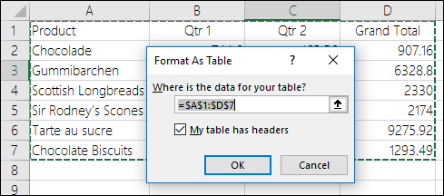
First row as header in excel - Word и Excel - помощь в работе с программами

With a cell in your table selected, click on the “Format as Table” option in the HOME menu. When the “Format As Table” dialog comes up, select the “My table has headers” checkbox and click the OK button. Select the first row; which should be your header row.

Contents

1 How do you make the first row heading?
2 How can you create the first row of the table as the header of the table?
3 How do I scroll first row in Excel?
4 How do you make first row in excel not numbered?
5 Why does my table not repeat header row?
6 Where is the header row in Excel?
7 How do I make headers in Excel?
8 How do I keep the first row in Excel always visible?
9 How do I keep the first row in sheets visible when scrolling?
10 How do I insert a specific row in Excel?
11 How do I number the first column in Excel?
12 How do I format a text header in Excel?
13 How do I put a header on every page?
14 Why is my header not showing up on all pages?
15 How do I change the header on each page?
16 How do I create a column header row in Excel?
17 What is Start row in Excel?
18 Why can’t I see the first row in Excel?
19 How do I keep the title row when scrolling in Excel?
20 How do I freeze both the top row and first column in Excel?

How do you make the first row heading?

To confirm that Power Query recognized your headers in the top row, select Home > Transform, and then select Use first row as headers. Power Query converts the first row of data to a header row. To return to the original headers, you can delete that step.

In the table, right-click in the row that you want to repeat, and then click Table Properties. In the Table Properties dialog box, on the Row tab, select the Repeat as header row at the top of each page check box.

How do I scroll first row in Excel?

How to freeze the top row in Excel

Scroll your spreadsheet until the row you want to lock in place is the first row visible under the row of letters.
In the menu, click “View.”
In the ribbon, click “Freeze Panes” and then click “Freeze Top Row.”

How do you make first row in excel not numbered?

Start row numbering at 0 instead of 1 in Excel

Create a new worksheet in your workbook.
In the new worksheet, select the Cell A2, enter the formula =ROW()-2, and drag the AutoFill handle down as many cells as possible.

Make sure that your long table is actually a single table. If it is not, then the header row won’t repeat because the table doesn’t really extend beyond a single page.multiple tables is to click somewhere within the table. Then, from the Layout tab of the ribbon, use the Select drop-down list to choose Table.

Row header or Row heading is the gray-colored column located on the left side of column 1 in the worksheet, which contains the numbers (1, 2, 3, etc.) where it helps out to identify each row in the worksheet.

How to add header in Excel

Go to the Insert tab > Text group and click the Header & Footer button.
Now, you can type text, insert a picture, add a preset header or specific elements in any of the three Header boxes at the top of the page.
When finished, click anywhere in the worksheet to leave the header area.

How do I keep the first row in Excel always visible?

To freeze the top row or first column:

From the View tab, Windows Group, click the Freeze Panes drop down arrow.
Select either Freeze Top Row or Freeze First Column.
Excel inserts a thin line to show you where the frozen pane begins.

How do I keep the first row in sheets visible when scrolling?

To pin data in the same place and see it when you scroll, you can freeze rows or columns.

On your computer, open a spreadsheet in Google Sheets.
Select a row or column you want to freeze or unfreeze.
At the top, click View. Freeze.
Select how many rows or columns to freeze.

How do I insert a specific row in Excel?

Insert rows

Select the heading of the row above where you want to insert additional rows. Tip: Select the same number of rows as you want to insert.
Hold down CONTROL, click the selected rows, and then on the pop-up menu, click Insert. Tip: To insert rows that contain data, see Copy and paste specific cell contents.

How do I number the first column in Excel?

Type 1 into a cell that you want to start the numbering, then drag the autofill handle at the right-down corner of the cell to the cells you want to number, and click the fill options to expand the option, and check Fill Series, then the cells are numbered.

On the status bar, click the Page Layout View button. Select the header or footer text you want to change. On the Home tab in the Font group, set the formatting options that you want to apply to the header / footer.

Use headers and footers to add a title, date, or page numbers to every page in a document.
Try it!

Select Insert > Header or Footer.
Select one of the built in designs.
Type the text you want in the header or footer.
Select Close Header and Footer when you’re done.

Hover the mouse over the top or bottom edge of any page until Word displays the white space arrows. Then, double-click the edge and Word will hide the header (and footer) and the white space.Uncheck the Show White Space Between Pages in Page Layout View option. Click OK.

Change or delete a header or footer on a single page

Double-click the first page header or footer area.
Check Different First Page to see if it’s selected. If not: Select Different First Page.
Add your new content into the header or footer.
Select Close Header and Footer or press Esc to exit.

How do I create a column header row in Excel?

Open the Spreadsheet

Open the Spreadsheet.
Open the spreadsheet where you want to have Excel make the top row a header row.
Add a Header Row.
Enter the column headings for your data across the top row of the spreadsheet, if necessary.
Select the First Data Row.

What is Start row in Excel?

You can get the first row (i.e. the starting row number) in a range with a formula based on the ROW function. In the example shown, the formula in cell F5 is: =MIN(ROW(data)) where data is a named range for B5:D10. When given a single cell reference, the ROW function returns the row number for that reference.

Why can’t I see the first row in Excel?

Select the Home tab from the toolbar at the top of the screen. Select Cells > Format > Hide & Unhide > Unhide Rows. Row 1 should now be visible in the spreadsheet.Try hiding rows 1-3 (even if they were hidden) and then try unhiding them again.

How do I keep the title row when scrolling in Excel?

To keep the column headers viewing means to freeze the top row of the worksheet.

Enable the worksheet you need to keep column header viewing, and click View > Freeze Panes > Freeze Top Row.
If you want to unfreeze the column headers, just click View > Freeze Panes > Unfreeze Panes.

How do I freeze both the top row and first column in Excel?

To freeze the top row and the first column at the same time, click the View tab > Freeze Panes > Freeze Panes.

Источник

Home / Excel Basics / How to Make First Row Header in Excel

In Excel, headers are a very important part of data structure, making the data easier to read and understand.

It helps users to understand what kind of data the cells will have under different columns based on the header’s names.

So, everyone who works in Excel knows the importance of having the first row of your data set as a header row.

This tutorial will explain how to make the first row of your data a header row.

By applying Freeze to the first row of the data set, the first row will get frozen as the header row, and when you scroll downwards in the spreadsheet, the first header row will get visible all the time.

First, open the data in the spreadsheet, where you want to freeze the first row as the headers row.
After that, go to the “View” tab and click on the “Freeze Panes” icon and then click on the “Freeze Top Row” option from the drop-down menu.
Or use the keyboard short “Alt → W → F → R” in sequence to directly choose the “Freeze Top Row” option.
At this moment, your first row got frozen as the headers row, and when you scroll down the Excel sheet, the headers will get visible all the time.

You can convert your data set into table format and make the first row a headers row by following the below steps:

First, go to any cell within the data and then go to the “Home” tab.
After that click on the “Format as Table” icon and choose the table format design.
Once you choose the table format or press the keyboard short “Ctrl + T” together, you will get the “Create Table” dialog box opened.
Now, you will see your data range is automatically got selected and you just select the “My table has headers” option and click OK.
At this moment, data will get converted into the table format with the first row as the headers row with filter icons.

You can use the Power Query Editor to make the first row of your data set the headers row by following the below steps:

First, go to any cell within the data set and go to the “Data” tab and there click on the “From Table/Range” option.
After that, see the selected range if it covered your whole data set, then un-select the “My table has headers” option and click OK.
Now, under the “Home” tab, click on the “Use First Row as Header” drop-down icon and then select the first option “Use First Row as Headers”.
Once you click on “Use First Row as Headers”, it will convert the first row of your data as headers.
In the end, click on the “Close & Load” icon and then click on the “Close & Load” option from the drop-down menu.
Once you click on the “Close & Load” option, your data will get transferred to a new sheet within the same workbook with the first row as headers.

Many times, you need to make the first row of your data set the headers row and you want to print that headers row on each page while printing the data. Follow the below steps for the same:

First, go to the “Page Layout” tab and then click on the “Print Titles” option and it will open the “Page Setup” dialog box.
After that, go to the “Rows to repeat at top” field and select the first header row, and then click on the “Print Preview” button to view if the headers are properly visible on the pages.
In the end, go to the “File” tab and click on the “Print” option or use the keyboard shortcut “Ctrl +P” to go to the “Print” dialog box to print the pages.

Источник

Excel for Microsoft 365 Excel for Microsoft 365 for Mac Excel for the web Excel 2021 Excel 2021 for Mac Excel 2019 Excel 2019 for Mac Excel 2016 Excel 2016 for Mac Excel 2013 Excel 2010 Excel 2007 Excel for Mac 2011 More…Less

When you create an Excel table, a table Header Row is automatically added as the first row of the table, but you have to option to turn it off or on.

When you first create a table, you have the option of using your own first row of data as a header row by checking the My table has headers option:

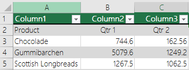
If you choose not to use your own headers, Excel will add default header names, like Column1, Column2 and so on, but you can change those at any time. Be aware that if you have a header row in your data, but choose not to use it, Excel will treat that row as data. In the following example, you would need to delete row 2 and rename the default headers, otherwise Excel will mistakenly see it as part of your data.

Notes:

The screen shots in this article were taken in Excel 2016. If you have a different version your view might be slightly different, but unless otherwise noted, the functionality is the same.
The table header row should not be confused with worksheet column headings or the headers for printed pages. For more information, see Print rows with column headers on top of every page.
When you turn the header row off, AutoFilter is turned off and any applied filters are removed from the table.
When you add a new column when table headers are not displayed, the name of the new table header cannot be determined by a series fill that is based on the value of the table header that is directly adjacent to the left of the new column. This only works when table headers are displayed. Instead, a default table header is added that you can change when you display table headers.
Although it is possible to refer to table headers that are turned off in formulas, you cannot refer to them by selecting them. References in tables to a hidden table header return zero (0) values, but they remain unchanged and return the table header values when the table header is displayed again. All other worksheet references (such as A1 or RC style references) to the table header are adjusted when the table header is turned off and may cause formulas to return unexpected results.

Show or hide the Header Row

Click anywhere in the table.
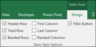
Go to Table Tools > Design on the Ribbon.
In the Table Style Options group, select the Header Row check box to hide or display the table headers.
If you rename the header rows and then turn off the header row, the original values you input will be retained if you turn the header row back on.

Notes:

The screen shots in this article were taken in Excel 2016. If you have a different version your view might be slightly different, but unless otherwise noted, the functionality is the same.
The table header row should not be confused with worksheet column headings or the headers for printed pages. For more information, see Print rows with column headers on top of every page.
When you turn the header row off, AutoFilter is turned off and any applied filters are removed from the table.
When you add a new column when table headers are not displayed, the name of the new table header cannot be determined by a series fill that is based on the value of the table header that is directly adjacent to the left of the new column. This only works when table headers are displayed. Instead, a default table header is added that you can change when you display table headers.
Although it is possible to refer to table headers that are turned off in formulas, you cannot refer to them by selecting them. References in tables to a hidden table header return zero (0) values, but they remain unchanged and return the table header values when the table header is displayed again. All other worksheet references (such as A1 or RC style references) to the table header are adjusted when the table header is turned off and may cause formulas to return unexpected results.

Show or hide the Header Row

Click anywhere in the table.
Go to the Table tab on the Ribbon.
In the Table Style Options group, select the Header Row check box to hide or display the table headers.
If you rename the header rows and then turn off the header row, the original values you input will be retained if you turn the header row back on.

Show or hide the Header Row

Click anywhere in the table.
On the Home tab on the ribbon, click the down arrow next to Table and select Toggle Header Row.

—OR—

Click the Table Design tab > Style Options > Header Row.

Need more help?

You can always ask an expert in the Excel Tech Community or get support in the Answers community.

Things You Should Know

Freeze a row by going to View > Freeze Panes.
Print a row across multiple pages using Page Layout > Print Titles.
Create a table with headers with Insert > Table. Select My table has headers.
Add headers to a Power Query table: Query > Edit > Transform > Use First Row as Headers.

1
Select a cell in the row you want to freeze. You can set Excel to freeze your header row so it’s always visible, even as you scroll.
- If your header row is in row 1, you don’t have to click any cells. Just continue to the next step.
- If your header row is down further, such as in row 2 or 3, click a cell below the header row.
  - For example, if the row that contains your column labels is row 5, you will need to click a cell in row 6.
2

Click the View tab. You’ll see it at the top of the window.

Advertisement
3

Click Freeze Panes. This menu is in the toolbar at the top of Excel. A list of freezing options will appear.
4
Select a Freeze Pane option. The option you select on this menu depends on whether your header row is in row 1 or in a different row:
- If your header row is in row 1 (the first row on your sheet), select Freeze Top Row. This ensures that the top row of your sheet remains locked into position, even as you scroll through your data.
- If your header row is in a different row, such as row 3, select Freeze Panes. This freezes the row above the cell you selected in Step 1.
  - For example, if you selected A6 in Step 1, selecting Freeze Panes will freeze row 5, making it your header row. This row will always stay visible as you scroll through your data.
- The Freeze Panes option works as a toggle. That is, if you already have panes frozen, clicking the option again will unfreeze your current setup. Clicking it a second time will refreeze the panes in the new position.
5

Add emphasis to your header row (optional). Create a visual contrast for this row by centering the text in these cells, applying bold text, adding a background color, or drawing a border under the cells. this can help the reader take notice of the header when reading the data on the sheet.

1

Click the Page Layout tab. If you have a large worksheet that spans multiple pages that you need to print, you can set a row or rows to print at the top of every page.
2

Click the Print Titles button. You’ll find this in the Page Setup section.
3

Set your Print Area to the cells containing the data. Click the button next to the Print Area field and then drag the selection over the data you want to print. Don’t include the column headers or row labels in this selection.
4

Click the button next to «Rows to repeat at top.» This will allow you to select the row(s) that you want to treat as the constant header.
5

Select the row(s) that you want to turn into a header. The rows that you select will appear at the top of every printed page. This is great for keeping large spreadsheets readable across multiple pages.
6

Click the button next to «Columns to repeat at left.» This will allow you to select columns that you want to keep constant on each page. These columns will act like the rows you selected in the previous step, and will appear on every printed page.
7
Set a header or footer (optional). You can include the company title or document title at the top, and insert page numbers at the bottom. This will help the reader get the pages organized. To set the header and footer:
- Click the Header/Footer tab
- Click the Header or Footer drop down menus to select a preset header.
- Alternatively, click Custom Header or Custom Footer to create your own.
8
Print your sheet. You can send the spreadsheet to print now, and Excel will print the data that you set with the constant header and columns you chose in the Print Titles window.
- Click Print to start the printing process.
- Check the print preview in the preview section.
- Click Print (the printer icon) to print the spreadsheet.

1
Select the data that you want to turn into a table. When you convert your data to a table, you can use the table to manipulate the data. One of the features of a table is the ability to set headers for the columns. Note that these are not the same as worksheet column headings or printed headers.
- For example, if you’re using Excel to track your bills, you might have headers like Date, Expense Type, and Amount.
2
Click the Insert tab and click Table. Confirm that your selection is correct.
- If you’re looking for Pivot Table information, check out our intro guide here.
3
Check the «My table has headers» box and click OK. This will create a table from the selected data. The first row of your selection will automatically be converted into column headers.
- If you don’t select «My table has headers,» a header row will be created using default names. You can edit these names by selecting the cell.
4
Enable or disable the header. This will show or hide the header. It won’t delete the header information, so you can turn it on and off as needed.^[1]
- Click the Design tab
- Check or uncheck the «Header Row» box to toggle the header row on and off. You can find this option in the Table Style Options section of the Design tab.
- Note that turning the header off will also remove any applied filters from the table.

1
Select a cell in your imported data. This will cause the “Table Design” and “Query” tabs to appear at the top of Excel. This method is used to add row headers to the dataset you imported using Get & Transform (Power Query). You’ll also be able to rename existing headers using this method.^[2]
- Note that this method requires the first row of your dataset to contain column header names.
2

Click Query. This is the rightmost tab at the top of Excel.
3

Click Edit in the Query tab. This is the icon with a spreadsheet and pencil. The Power Query Editor window will open.
4

Click Transform. This is a tab at the top of the Power Query Editor.
5
Make the first row of data the header. To do so:
- Click Use First Row as Headers.
- Select Use First Row as Headers in the drop down menu. This will make row 1 into the headers for the table.
6
Rename the headers. In the Power Query Editor, you can rename the column headers using these steps:
- Double-click the column header name.
- Type in a new name for the header.
- Press ↵ Enter to confirm the name.
7

Click Close & Load in the Home tab of the editor. This will reload the imported table with the changes you made in the editor.

Add New Question

Question

How do I get my headers to change the dates and days automatically?

Use the function @Today. You’ll find it near the top under the choice «Functions».

Ask a Question

200 characters left

Include your email address to get a message when this question is answered.

Submit

Most errors that occur from using the Freeze Panes option are the result of selecting the header row instead of the row just beneath it. If you receive an unintended result, remove the «Freeze Panes» option, select 1 row lower and try again.

Thanks for submitting a tip for review!

About This Article

Article SummaryX

1. Click the View tab.
2. Select the corner cell under the header row.
3. Click Freeze Panes.
4. Apply formatting to the header row.

Did this summary help you?

Thanks to all authors for creating a page that has been read 1,049,311 times.

Is this article up to date?

Источник

Introduction

Excel does not give an easy way of changing your column headings to something other than the built-in A, B, C or 1, 2, 3 (R1C1) format. However, if you format the entire table as a Table, then Excel has a useful trick to enable such a feature.

Enabling Customized Column Headers

Using Microsoft Excel 2013 or later (haven’t tried earlier versions), create a table in Excel.
Make the first row the header row that you wish to see in the columns by giving it short meaningful names.
With a cell in your table selected, click on the «Format as Table» option in the HOME menu.
When the «Format As Table» dialog comes up, select the «My table has headers» checkbox and click the OK button.
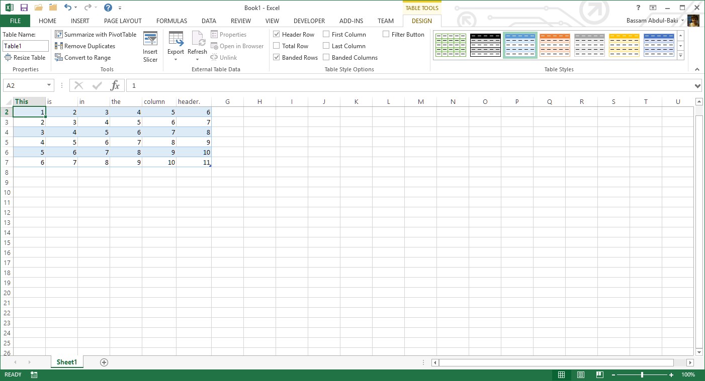
Select the first row; which should be your header row.
Right-click on the grey row 1 header area and select hide.
The column names for only the table area should now reflect the first row data.

Note: If you scroll down or right outside of the table area, the column headers switch to the built-in format.

Points of Interest

This feature did not work for row headers and only seems to work with the «Format as Table» option.

History

2017-05-21: Introduction

Bassam Abdul-Baki has a Bachelor of Science (BS) degree and a Master of Science (MS) degree in Mathematics and another MS in Technology Management. He’s an analyst by trade. He started out in Quality Assurance (QA) and analysis, then dabbled in Visual C++ and Visual C# programming for a while, and then came back to QA and analysis again. He’s not sure where he’ll be five years from now, but is looking into data analytics.

Bassam is into mathematics, technology, astronomy, archaeology, and genealogy.

Источник

How do you make the first row heading?

How do I scroll first row in Excel?

How do you make first row in excel not numbered?

How do I keep the first row in Excel always visible?

How do I keep the first row in sheets visible when scrolling?

How do I insert a specific row in Excel?

How do I number the first column in Excel?

How do I create a column header row in Excel?

What is Start row in Excel?

Why can’t I see the first row in Excel?

How do I keep the title row when scrolling in Excel?

How do I freeze both the top row and first column in Excel?

Show or hide the Header Row

Show or hide the Header Row

Show or hide the Header Row

Need more help?

See Also

Need more help?

Things You Should Know

About This Article

Is this article up to date?

Introduction

Enabling Customized Column Headers

Points of Interest

History