First last names excel

Let’s say you want to create a single Full Name column by combining two other columns, First Name and Last Name. To combine first and last names, use the CONCATENATE function or the ampersand (&) operator.

Important: In Excel 2016, Excel Mobile, and Excel for the web, this function has been replaced with the CONCAT function. Although the CONCATENATE function is still available for backward compatibility, you should consider using CONCAT from now on. This is because CONCATENATE may not be available in future versions of Excel.

Example

Copy the following example to a blank worksheet.

1 2 3

A B First Name Last Name Nancy Davolio Andrew Fuller Formula Description (Result) =A2&» «&B2 Combines the names above, separated by a space (Nancy Davolio) =B3&», «&A3 Combines the names above, separated by a comma (Fuller, Andrew) =CONCAT(A2,» «,B2) Combines the names above, separated by a space (Nancy Davolio)

Note: To replace the formula with the results, select the cells, and on the Home tab, in the Clipboard group, click Copy , click Paste , and then click Paste Values.

Need more help?

You can always ask an expert in the Excel Tech Community or get support in the Answers community.

Watch Video – Split Names in Excel (into First, Middle, and Last name)

Excel is an amazing tool when it comes to slicing and dicing text data.

There are so many useful formulas as well as functionalities you can use to work with text data in Excel.

One of the very common questions I get about manipulating text data is – “How to separate first and last names (or first, middle, and last names) in Excel?“.

There are a couple of easy ways to split names in Excel. The method you choose will depend on how your data is structured and whether you want cowothe result to be static or dynamic.

So let’s get started and see different ways to split names in Excel.

Split Names Using Text to Columns

Text to Columns functionality in Excel allows you to quickly split text values into separate cells in a row.

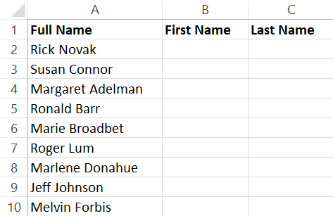
For example, suppose you have the dataset as shown below and you want to separate the first and last name and get these in separate cells.

Below are the steps to separate the first and last name using Text to Columns:

1. Select all the names in the column (A2:A10 in this example)
2. Click the ‘Data’ tab
3. In the ‘Data Tools’ group, click on the ‘Text to Columns’ option.
4. Make the following changes in the Convert Text to Column Wizard:
   1. Step 1 of 3: Select Delimited (this allows you to use space as the separator) and click on Next
   2. Step 2 of 3: Select the Space option and click on Next
   3. Step 3 of 3: Set B2 as the destination cell (else it will overwrite the existing data)
5. Click on Finish

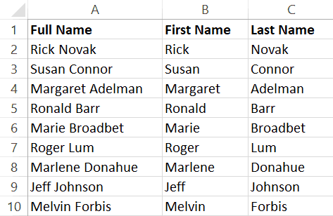
The above steps would instantly split the names into first and last name (with first names in column B and last name in column C).

Note: In case there is any data in the cells already (the ones where Text to Columns output is expected), Excel will show you a warning letting you know that there is some data already in the cells. You can choose to overwrite the data or cancel Text to Columns and manually remove it first.

Once done, you can delete the full name data if you want.

A few things to know when using Text to Columns to separate first and last names in Excel:

1. The result of this is static. This means that in case you have new data or the original data has some changes, you need to do this all over again to split the names.
2. If you only want the First name or only the Last name, you can skip the columns you don’t want in step 3 of the ‘Text to Column Wizard’ dialog box. To do this, select the column in the preview that you want to skip and then select the ‘Do not import column (skip)’ option.
3. In case you don’t specify the destination cell, Text to Column will overwrite the current column

Text to Columns option is best suited when you have consistent data (for example all names have first and last name only or all names have a first, middle, and last names).

In this example, I have shown you how to separate names that have space as the delimiter. In case the delimiter is a comma or a combination of comma and space, you can still use the same steps. In this case, you can specify the delimiter in Step 2 of 3 of the wizard. There is already an option to use the comma as the delimiter, or you can select ‘Other’ option and specify a custom delimiter as well.

While Text to Columns is a fast and efficient way to split names, it’s suited only when you want the output to be a static result. In case you have a dataset that may expand or change, you are better off using formulas to separate the names.

Separate First, Middle, and Last Names Using Formulas

Formulas allow you to slice and dice the text data and extract what you want.

In this section, I will share various formulas you can use to separate name data (based on how your data is structured).

Below are the three formulas you can use to separate first, middle, and last name (explained in detail later in the following sections).

Formula to get the first name:

=LEFT(A2,SEARCH(" ",A2)-1)

Formula to get the middle name:

=MID(A2,SEARCH(" ",A2)+1,SEARCH(" ",SUBSTITUTE(A2," ","@",1))-SEARCH(" ",A2))

Formula to get the last name:

=RIGHT(A15,LEN(A15)-SEARCH("@",SUBSTITUTE(A15," ","@",LEN(A15)-LEN(SUBSTITUTE(A15," ","")))))

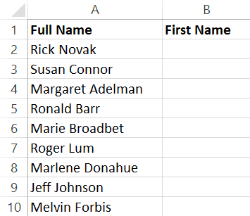
Get the First Name

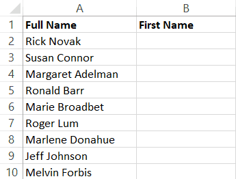
Suppose you have the dataset as shown below and you want to quickly separate the first name in one cell and last name in one cell.

The below formula will give you the first name:

=LEFT(A2,SEARCH(" ",A2)-1)

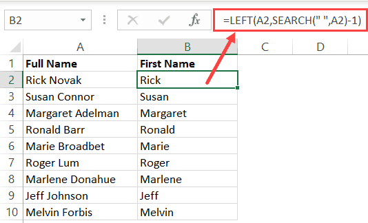
The above formula uses the SEARCH function to get the position of the space character in between the first and last name. The LEFT function then uses this space position number to extract all the text before it.

This is a fairly straight forward use of extracting a part of the text value. Since all we need to do is identify the first space character position, it doesn’t matter whether the name has any middle name or not. The above formula is going to work just fine.

Now, let’s get a little more advanced with each example.

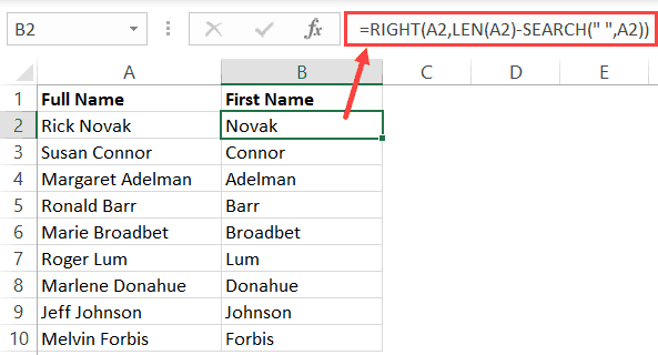
Get the Last Name

Let’s say you have the same dataset and this time you need to get the last name.

The below formula will extract the last name from the above dataset:

=RIGHT(A2,LEN(A2)-SEARCH(" ",A2))

Again, quite straightforward.

This time, we first find the space character position, which is then used to find out the number of characters that are left after space (which would be the last name).

This is achieved by subtracting the position value of the space character with the total number of characters in the name.

This number is then used in the RIGHT function to fetch all these characters from the right of the name.

While this formula works great when there is only the first and last name, it wouldn’t work in case you also have a middle name. This is because we only accounted for one space character (between first and last name). Having a middle name adds more space characters to the name.

To fetch the last name when you have a middle name as well, use the below formula:

=RIGHT(A15,LEN(A15)-SEARCH("@",SUBSTITUTE(A15," ","@",LEN(A15)-LEN(SUBSTITUTE(A15," ","")))))

Now, this has started to become a bit complex… isn’t it?

Let me explain how this works.

The above formula first finds the total number of space characters in the name. This is done by getting the length of the name with and without the space character and then subtracting the one without space from the one with space. This gives the total number of space characters.

The SUBSTITUTE function is then used to replace the last space character with an ‘@’ symbol (you can use any symbol – something which is unlikely to occur as a part of the name).

Once the @ symbol has been substituted in place of the last space character, you can easily find the position of this @ symbol. This is done using the SEARCH function.

Now all you need to do is extract all the characters to the right of this @ symbol. This is done by using the RIGHT function.

Get the Middle Name

Suppose you have the dataset as shown below and you want to extract the middle name.

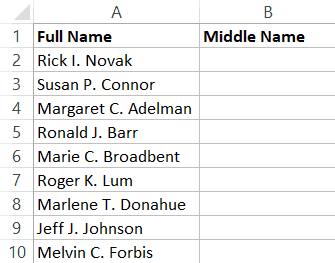
The following formula will do this:

=MID(A2,SEARCH(" ",A2)+1,SEARCH(" ",SUBSTITUTE(A2," ","@",1))-SEARCH(" ",A2))

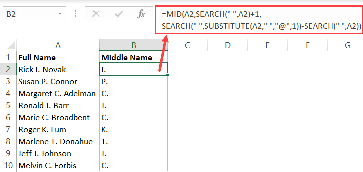
The above formula uses the MID function, which allows you to specify a start position and the number of characters to extract from that position.

The start position is easy to find using the SEARCH function.

The hard part is to find how many characters to extract after this start position. To get this, you need to identify how many characters are there from the start position to the last space character.

This can be done by using the SUBSTITUTE function and replace the last space character with an ‘@’ symbol. Once this is done, you can easily use the SEARCH function to find the position of this last space character.

Now that you have the starting position and the position of the last space, you can easily fetch the middle name by using the MID function.

One of the benefits of using a formula to separate the names is that the result is dynamic. So in case, your dataset expands and more names are added to it or if some names change in the original dataset, you don’t need to worry about the resulting data.

Separate Names Using Find and Replace

I love the flexibility that comes with ‘Find and Replace‘ – because you can use wild card characters in it.

Let me first explain what’s a wild card character.

A wildcard character is something that you can use instead of any text. For example, you can use an asterisk symbol (*) and it will represent any number of characters in Excel. To give you an example, if I want to find all the names that start with the alphabet A, I can use A* in find and replace. This will find and select all the cells where the name starts with A.

If you’re still not clear, don’t worry. Keep reading and the next few examples will make it clear what wildcard characters are and how to use these to quickly separate names (or any text values in Excel).

In all the examples covered below, make sure you create a backup copy of the dataset. Find and Replace changes the data on which it’s used. It’s best to copy and paste the data first and then use Find and Replace on the copied dataset.

Get the First Name

Suppose you have a dataset as shown below and you want to get the first name only.

Below are the steps to do this:

1. Copy the name data in Column A and paste it in Column B.
2. With the data in Column B selected, click the Home tab
3. In the Editing group, click on Find & Select.
4. Click on Replace. This will open the ‘Find and Replace’ dialog box.
5. In the ‘Find and Replace’ dialog box, enter the following
   1. Find what:  * (space character followed by the asterisk symbol)
   2. Replace with: leave this blank
6. Click on Replace All.

The above steps would give you the first name and remove everything after the first name.

This works even if you have names that have a middle name.

Pro Tip: The keyboard shortcut to open the Find and Replace dialog box is Control + H (hold the control key and then press the H key).

Get the Last Name

Suppose you have a dataset as shown below and you want to get the last name only.

Below are the steps to do this:

1. Copy the name data in Column A and paste it in Column B.
2. With the data in Column B selected, click the Home tab
3. In the Editing group, click on Find & Select.
4. Click on Replace. This will open the ‘Find and Replace’ dialog box.
5. In the ‘Find and Replace’ dialog box, enter the following
   1. Find what: *  (asterisk symbol followed by a space character)
   2. Replace with: leave this blank
6. Click on Replace All.

The above steps would give you the last name and remove everything before the first name.

This works even if you have names that have a middle name.

Remove the Middle Name

In case you only want to get rid of the middle name and only have the first and the last name, you can do that using Find and Replace.

Suppose you have a dataset as shown below and you want to remove the middle name from these.

Below are the steps to do this:

1. Copy the name data in Column A and paste it in Column B.
2. With the data in Column B selected, click the Home tab
3. In the Editing group, click on Find & Select.
4. Click on Replace. This will open the ‘Find and Replace’ dialog box.
5. In the ‘Find and Replace’ dialog box, enter the following
   1. Find what: * (space character followed by the asterisk symbol followed by the space character)
   2. Replace with:  (just put a space character here)
6. Click on Replace All.

The above steps would remove the middle name from a full name. In case some names don’t have any middle name, they would not be changed.

Separate Names Using Flash Fill

Flash fill was introduced in Excel 2013 and makes it really easy to modify or clean a text data set.

And when it comes to separating names data, it’s right up in Flash Fill’s alley.

The most important thing to know when using Flash Fill is that there needs to a pattern that flash fill can identify. Once it has identified the pattern, it will easily help you split names in Excel (you will get more clarity on this when you go through a few examples below).

Get the First or the Last Name from Full Name

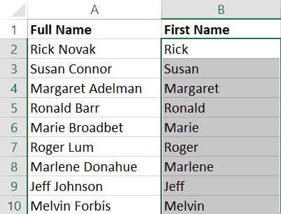
Suppose you have a dataset as shown below and you want to get only the first name.

1. In the adjacent cell, manually type the first name from the full name. In this example, I would type Rick.
2. In the second cell, manually type the first name from the adjacent cell’s name. While you’re typing, you will see Flash Fill show you a list of the first name automatically (in gray).
3. When you see the names in grey, quickly glance through it to make sure it’s showing the right names. If these are right, hit the enter key and Flash Fill will automatically fill the rest of the cells with the first name.

Flash Fill needs you to give it a pattern that it can follow when giving you the modified data. In our example, when you type the first name in the first cell, Flash Fill can’t figure out the pattern.

But as soon as you start entering the First name in the second cell, Flash Fill understands the pattern and shows you some a suggestion. If the suggestion is correct, just hit the enter key.

And if it’s not correct, you can try entering manually in a few more cells and check if Flash Fill is able to discern the pattern or not.

Sometimes, you may not see the pattern in gray (as shown in step 2 above). If that’s the case, follow the below steps to get the Flash Fill result:

1. Enter the text manually in two cells.
2. Select both these cells
3. Hover the cursor on the bottom-right part of the selection. You will notice that the cursor changes to a plus icon
4. Double click on it (mouse left-key). This will fill all the cells. At this point in time, the results are likely incorrect and not what you expected.
5. At the bottom right of the resulting data, you will see a small Auto-Fill icon. Click on this Auto-fill icon
6. Click on Flash Fill

The above steps would give you the result from Flash Fill (based on the pattern it has deduced).

You can also use Flash Fill to get the last name or the middle name. In the first two cells, enter the last name (or the middle name) and flash fill will be able to understand the pattern

Rearrange Name Using Flash Fill

Flash Fill is a smart tool and it can decipher slightly complex pattern as well

For example, suppose you have a dataset as shown below and you want to rearrange the name from Rick Novak to Novak, Rick (where the last name comes first followed by a comma and then the first name).

Below are the steps to do this:

1. In the adjacent cell, manually type Novak, Rick
2. In the second cell, manually type Connor, Susan. While you’re typing, you will see Flash Fill show you a list of the names in the same format (in gray).
3. When you see the names in grey, quickly glance through it to make sure it’s showing the right names. If these are right, hit the enter key and Flash Fill will automatically fill the rest of the cells with the names in the same format.

Remove the Middle Name (or Just get the middle name)

You can also use Flash Fill to get rid of the middle name or get only the middle name.

For example, suppose you have a dataset as shown below and you want to get only the first and the last name and not the middle name.

Below are the steps to do this:

1. In the adjacent cell, manually type Rick Novak
2. In the second cell, manually type Susan Connor. While you’re typing, you will see Flash Fill show you a list of the names in the same format (in gray).
3. When you see the names in grey, quickly glance through it to make sure it’s showing the right names. If these are right, hit the enter key and Flash Fill will automatically fill the rest of the cells with the names without the middle name.

Similarly, if you only want to get the middle names, type the middle name in the first two cells and use Flash Fill to get the middle name from all the remaining names.

The examples shown in this tutorial uses names while manipulating the text data. You can use the same concepts to also work with other formats of data (such as addresses, product names, etc.)

You may also like the following Excel tutorials:

• Extract Usernames from Email Ids in Excel
• How to Filter Cells that have Duplicate Text Strings (Words) in it
• Convert Date to Text in Excel
• Convert Text to Numbers in Excel
• How to Remove the First Character from a String in Excel
• How to Sort by the Last Name in Excel
• How to Combine First and Last Name in Excel
• Extract Last Name in Excel (5 Easy Ways)
• Separate Text and Numbers in Excel
• How to Switch First and Last Name in Excel with Comma?

Often we face a situation where we need to separate names (get the first and last word from a cell/text string) in Excel.

Let’s say you want to extract the first name from a cell where you have both first and last names or you want to extract the product name from the product description cell.

We do need a function that can extract this. The bad news is, in Excel, there is no specific function to extract the first and the last word from a cell directly.

But the good news is you can combine functions and create a formula to get these words. Today in this post, I’d like to share with you how to get separate names using a formula

sample-file

Extracting the first word from a text string is much easier than extracting the last word. For this, we can create a formula by combining two different text functions, that’s SEARCH and LEFT.

Let’s understand this with an example. In the below table, we have a list of names which includes the first and the last name. And now from this, we need to extract the first name which is the first word in the cell.

And the formula to get the first name from the above column is:

=LEFT(A2,SEARCH(" ",A2)-1)

This simply returns the first name which is the first word from the text.

How it Works

In the above example, we have used a combination of SEARCH (It can search for a text string in another text string) and LEFT (It can extract a text from the left side).

This formula works in two different parts.

In the first part, the SEARCH function finds the position of the space in the text and returns a number from which you have deducted one to get the position of the last character of the first word.

In the second part, using the number returned by the SEARCH function, the LEFT function extracts the first word from the cell.

Getting the last word from a text string can be tricky for you, but once you understand the entire formula it will be much easier to use it in the future.

So, to extract the last word from a cell you need to combine RIGHT, SUBSTITUTE, and REPT. And the formula will be:

=TRIM(RIGHT(SUBSTITUTE(A2," ",REPT(" ",LEN(A2))),LEN(A2)))

This formula returns the last name from the cell which is the last word and works the same even if you have more than two words in a cell.

How it Works

Again, you need to break down this formula to understand how it works.

In the FIRST part, the SUBSTITUTE function replaces every single space with spaces equal to the length of the text.

The text becomes double in length with extra spaces and looks something like this. After that, the RIGHT function will extract characters from the right side equal to the original length of the text.

In the end, the TRIM function removes all the leading spaces from the text.

sample-file

Conclusion

By using the above formulas you can easily get the first and the last word from a text string.

The formula for the first word is super easy and for the last word is a bit tricky but you need to understand it once it starts.

I hope you found this tip helpful.

Now tell me one thing. Do you have any other method to get first and last from a string? Please share your views with me in the comment section, I’d love to hear from you. And, please don’t forget to share this tip with your friends.

Do you need to switch the first and last names with a comma?

One of the issues in dealing with contact data is the format of their full name. For contacts whose full name appears as First Last, you would likely rather format it as Last, First.

Doing so usually leads to easier sorting and filtering in your list. Also, last names are generally more unique than first names which makes any lookups more reliable.

This post explores several different ways to reverse the first and last names in Excel.

Switch First and Last Names with Text to Columns

One way to switch first and last names is through a feature called Text to Columns.

This feature can separate first and last names into their own cells, where they can be re-combined into the new format using a formula.

To get started, select the cells containing your contacts.

Go to the Data ribbon tab and click Text to Columns.

Ensure Delimited is chosen as your Original data type. This is because the space character acts as a separator between the first and last name.

Click the Next button when ready.

Out of the above Delimiters, check the Space option as your delimiter and clear all the other Delimiters checkboxes.

The Data preview shows how Excel will separate the names.

Click the Next button.

Select the Destination textbox, then select one cell that will be the starting point of your separated names.

In the above example, the first name of your first contact will go into the cell $C$3 while the last name will go into the adjacent right cell. The rest of your contacts will get separated similarly going downward.

Click the Finish button.

As you can see above, the first and last names have been separated into their own columns.

= D3 & ", " & C3

The next step is to re-combine the columns to switch the names.

In the row of your first contact, select an empty cell and paste the above formula into the formula bar.

The ampersand (&) joins the last name from cell D3 with the first name from cell C3 and separates them with a comma (,) in between.

Press Enter to calculate the formula.

To apply the formula to the other contacts, hover over the lower-right corner of the formula’s cell until your cursor becomes a plus (+), then left-click and hold your mouse button while dragging downward.

Your contact names are now switched!

Switch First and Last Names with Text Formula

If you’d rather use a formula-only solution to switch names, there is a way to do it.

Such a formula will append results from the FIND, LEN, RIGHT and LEFT functions to format each name into a new cell.

FIND ( " " , B3 )

Given a full name in cell B3, the above FIND function returns the position of the space character, starting from the left.

LEN ( B3 ) - FIND ( " " , B3 )

To calculate the position of the space character starting from the right, the FIND result is subtracted from the length of the full name.

RIGHT ( B3 , LEN ( B3 ) - FIND ( " " , B3 ) )

The last name is extracted using the above RIGHT function.

LEFT ( B4 , FIND ( " " , B4 ) - 1 )

Extracting the first name is similar, as shown above. But 1 is subtracted from the FIND result so that the space character gets excluded.

= RIGHT ( B3, LEN ( B3 ) - FIND ( " ", B3 ) ) & ", " & LEFT ( B3 , FIND ( " " , B3 ) - 1 ) 

Putting all of this together, paste the above formula into the empty cell to the right of your first contact. The formula joins together the last and first name, with a comma (,) in between.

Press Enter to trigger the formula calculation.

To apply the formula to your other contacts, hover over the lower-right corner of the formula’s cell until your cursor becomes a plus (+), then left-click and hold your mouse button while dragging downward.

Voila! Your name formatting is complete!

Switch First and Last Names with TEXTSPLIT Function

TEXTSPLIT is a new function introduced in Excel 365 beta version 2203.

The TEXTSPLIT function separates a cell value into multiple cell values. It gives you the functionality of the Text to Columns feature but through a formula.

TEXTSPLIT ( B3 , " " )

The above TEXTSPLIT finds the space character within the contact in cell B3. All characters to the left of the space are extracted as one item, as are all characters to the right.

The result is a two-item array holding the first name followed by the last name.

SEQUENCE ( COUNTA ( TEXTSPLIT ( B3 , " " ) ) )

The COUNTA function counts the number of array items, which for most names will be two.

The SEQUENCE function uses that count to create a two-item array of sequenced numbers. This is what will be used to reverse the order of the names.

SORTBY ( TRANSPOSE ( TEXTSPLIT ( B3 , " " ) ) , SEQUENCE ( COUNTA ( TEXTSPLIT ( B3 , " " ) ) ) , -1 )

Both arrays are supplied to the SORTBY function which rearranges the names as a result of their corresponding numbers.

The -1 enforces the sort as reversed, effectively switching the names!

TRANSPOSE is required because SORTBY expects the names array to be vertically populated like the numbers array.

= TEXTJOIN ( ", " , TRUE , SORTBY ( TRANSPOSE ( TEXTSPLIT ( B3 , " " ) ) , SEQUENCE ( COUNTA ( TEXTSPLIT ( B3 , " " ) ) ) , -1 ) )

The final version of the formula is above. Paste this version into your formula bar.

The above TEXTJOIN function converts the array of switched names into a single full name, including the embedded comma (,).

The only step left is to copy the formula to the other contacts. Hover over the lower-right corner of the formula’s cell until your cursor becomes a plus (+), then left-click and hold your mouse button while dragging downward.

You now have all your contacts’ names flipped with a comma in between!

Switch First and Last Names with Flash Fill

The Flash Fill feature is a great way to switch first and last names without having to write complex formulas.

By providing some examples of switched names, Flash Fill can learn from your examples and automatically switch your remaining names!

Start a Flash Fill by first selecting the empty cell to the right of your first contact. In that cell, type the contact’s name with the first and last names switched. Then press Enter.

Ensure that the active cell is still within the column of your example.

Go to the Data ribbon tab and click Flash Fill, or simply press Ctrl + E.

Magically, Flash Fill recognizes that you want first and last names switched and will offer you a preview of the results!

To accept the results, click the Flash Fill Options menu at the lower-right corner of your cell, then click Accept suggestions.

You are all done and the names are all reversed!

Switch First and Last Names with Power Query

Power Query is a feature of Excel that allows you to perform complex transformations on your data.

To switch first and last names, you can give Power Query some examples and once the pattern is recognized, Power Query will finish the task for you and create the formulas required for the transform!

To launch Power Query, first select your column of contacts, including your header.

Go to the Data ribbon tab and click From Table/Range.

From the Power Query Editor window, go to the Add Column tab, then click Column From Examples.

You need to provide enough examples for Power Query to recognize the switch pattern.

Type your first example in the first row of the right column. For example, if your first contact is “Trent Buckston”, type “Buckston, Trent”, as shown above.

Press Enter after typing.

📝 Note: You don’t need to provide examples in order starting with the first row. You can the examples in any rows.

Type a second example in the second row to further help Power Query.

Again, press Enter after typing.

Notice above how Power Query uses your examples to guess the remaining rows. The results are not exactly what you want, so you need to provide additional examples.

After you provide your third example, you will finally see the desired results!

Select the Custom column header and type a descriptive name such as Switched, then press Enter and click the OK button.

Note above that the original Full Name column still appears. Because you already have the Full Name column on your sheet, you can remove that column.

Select the column and go to the Home tab then click on the Remove Columns command.

Place the Switched column onto your sheet by clicking the Close & Load dropdown, then Close & Load To.

From the Import Data window, select the Table option and choose Existing worksheet. Highlight its textbox contents and select an empty cell on your sheet. This cell will become the first row of your results.

When done, click the OK button.

As you can see above, your column of switched names now appears on your sheet!

Switch First and Last Names with Power Pivot

Power Pivot is an add-in for Excel that adds business intelligence to large amounts of data.

With Power Pivot, you can add a calculated column of switched names, then display that column with a pivot table.

By default, Power Pivot is disabled in Excel. But you can enable it to add the Power Pivot tab to your Excel ribbon.

Select your contact data, go to the Power Pivot ribbon tab and click Add to Data Model.

Your contact data now appears as a table column in Power Pivot. It is helpful to give this table a more descriptive name by double-clicking the bottom tab and renaming it Names.

Press Enter when done.

= RIGHT( Names[Full Name] , LEN( Names[Full Name] ) - FIND( " " , Names[Full Name] ) ) & ", " & LEFT( Names[Full Name] , FIND( " " , Names[Full Name] ) - 1 )

To create the column of switched names, select the column labeled Add column.

Paste the above formula into the formula bar. This formula performs the same actions as the text formula solution seen earlier in this post.

The key difference is that Power Pivot uses a formula language called DAX to reference an entire column at once!

For example, the formula references the Full Name column of the Names table using the Names[Full Name] syntax.

After you press Enter, all your switched names appear in the new column!

Give your new column a more descriptive name by double-clicking the column header and typing Switched.

Press Enter when done.

You are now ready to display the new column on your sheet. Go to the Home tab and click PivotTable.

Choose a destination for your Pivot Table. In the above example, a new worksheet will be created.

Click the OK button when ready.

In the PivotTable Fields pane, drill into the Names table and check the Switched field, so that the field appears in the Rows area.

Your switched names are now on your sheet inside a pivot table!

Switch First and Last Names with VBA

Excel’s VBA programming language offers you a highly automated, sophisticated solution to switching your names.

Through VBA, you can create code that iterates over each contact and then separates and re-joins their name in reverse order before outputting it to a new column.

To add such code to your workbook, open the VBA Editor by pressing Alt + F11.

It is a good idea to keep your custom code separate from the workbook itself, so create a module by selecting the Insert menu, then selecting Module.

Sub SplitNames()
Dim rng As Range
Dim arrNames() As String
Dim colCount As Integer

colCount = Selection.Columns.Count
If colCount <> 1 Then
    MsgBox ("Select a single column!")
    End
End If

For Each rng In Selection
    arrNames = Split(rng.Value, " ")
    rng.Offset(0, 1).Value = arrNames(1) & ", " & arrNames(0)
Next rng
End Sub

Double-click the new module to open it, then paste the above VBA code into the module.

At run-time, the above code first ensures that you’ve selected only one column of contacts on your sheet. Any other selection causes execution to end with a notification.

The code loops through each selected cell and separates the first and last names. The separation occurs at the position of the space character via the Split function.

Both names are placed in an array called arrNames. The array elements are re-joined in reverse order using the ampersand (&) and placed in the adjacent cell represented by rng.Offset(0, 1).

VBA code such as this is often referred to as a macro when it can be run from your sheet.

To run this macro, go back to your sheet and ensure you’ve selected your column of contacts.

Select the View ribbon tab and click Macros.

From the Macro dialog, select your SplitNames macro and click the Run button.

When the run finishes, you can see the adjacent column now contains your contacts with reversed names!

Switch First and Last Names with Office Scripts

With the advent of Microsoft 365 for the web, a new scripting language called Office Scripts is available to business plan users of Excel.

You can take advantage of Office Scripts to automate tasks like the switching of first and last names.

To start your own script, open your workbook from your web browser.

Select the Automate ribbon tab, then click New Script.

If you don’t see the Automate tab, check your Microsoft 365 license to ensure that you have the required business plan to access Office Scripts and that it’s been enabled in your admin settings.

function main(workbook: ExcelScript.Workbook) {

  //getselected range
  let rng = workbook.getSelectedRange();
  let rows = rng.getRowCount();
  let cols = rng.getColumnCount();

  if (cols != 1) {
    return;
  };

  //loop through selected cells
  for (let i = 0; i < rows; i++) {
    for (let j = 0; j < cols; j++) {
      //split name based on space
      let txtName = rng.getCell(i, j).getValue().toString();
      let arrName = txtName.split(" ");
      //enter names in adjacent cells
      rng.getCell(i, j + 1).setValue(arrName[1] + ", " + arrName[0]);
    };
  };
};

In the Code Editor pane that appears, replace its entire contents with the above script.

📝 Note: You always need a main function in your script because that is the starting point of every script.

This script first ensures that you have only one column of contacts selected, otherwise the script terminates.

The script loops through each contact. The first and last names get extracted by finding the position of the space character.

The two names get re-combined in reverse order with a comma (,) in between. The result gets placed into the adjacent cell before processing the next contact.

Before running your script, go to your sheet and select your column of contacts.

Click the Run button in the Code Editor pane to execute the code.

When it finishes, you can see the adjacent column now has the contacts with their names switched!

Conclusions

In this post, you’ve seen many ways to switch first and last names in Excel.

The Text to Columns feature offers a clean, interactive experience, whereas the text formula method benefits from fewer steps and the results will dynamically update if the source names change.

The formula involving TEXTSPLIT exposes you to the benefits of Excel’s dynamic array functions. But keep in mind not all users will have this function.

The Flash Fill feature is great for patterned tasks like switching names but may fall short when your data is inconsistently formatted.

For larger data sources, you could choose Power Query or Power Pivot. Power Query requires less formula knowledge with the powerful column by example feature.

Otherwise, you have VBA and Office Scripts as flexible coding options depending on if you work with the desktop app or the online app.

Have you needed to switch names in Excel? How did you get it done? Let me know in the comments.

To extract the first, middle and last name we use the formulas «LEFT», «RIGHT», «MID», «LEN», and «SEARCH» in Excel.

LEFT: Returns the first character(s) in a text string based on the number of characters specified.

Syntax of «LEFT» function: =LEFT (text,[num_chars])

Example:Cell A2 contains the text «Mahesh Kumar Gupta»
=LEFT (A2, 6), function will return «Mahesh»

RIGHT:Return the last character(s) in a text string based on the number of characters specified.

Syntax of «RIGHT» function: =RIGHT (text, [num_chars])

Example:Cell A2 contains the text «Mahesh Kumar Gupta»
=RIGHT (A2, 5), function will return «GUPTA»

MID:Return a specific number of character(s) from a text string, starting at the position specified based on the number of characters specified.

Syntax of «MID» function: =MID (text,start_num,num_chars)

Example:Cell A2 contains the text «Mahesh Kumar Gupta»
=MID (A2, 8, 5), function will return «KUMAR»

LEN:Returns the number of characters in a text string.

Syntax of «LEN» function: =LEN (text)

Example:Cell A2 contains the text «Mahesh Kumar Gupta»
=LEN (A2), function will return 18

SEARCH:The SEARCH function returns the starting position of a text string which it locates from within the text string.

Syntax of «SEARCH» function: =SEARCH (find_text,within_text,[start_num])

Example:Cell A2 contains the text «Mahesh Kumar Gupta»
=SEARCH («Kumar», A2, 1), function will return 8

How to separating the names in Excel through formula? 

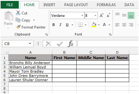
To understand how you can extract the first, middle and last name from the text follow the below mentioned steps:

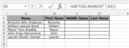
Example 1: We have a list of Names in Column “A” and we need to pick the First name from the list. We will write the «LEFT» function along with the «SEARCH» function.

• Select the Cell B2, write the formula =LEFT (A2, SEARCH (» «, A2)), function will return the first name from the cell A2.
• To Copy the formula in all cells press the key “CTRL + C” and select the cell B3 to B6 and press the key “CTRL + V” on your keyboard.

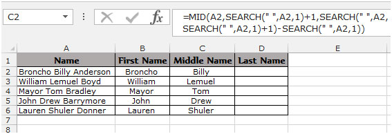
To pick the Middle name from the list. We write the “MID” function along with the “SEARCH” function.

• Select the Cell C2, write the formula =MID(A2,SEARCH(» «,A2,1)+1,SEARCH(» «,A2,SEARCH(» «,A2,1)+1)-SEARCH(» «,A2,1)) it will return the middle name from the cell A2.
• To Copy the formula in all cells press key “CTRL + C” and select the cell C3 to C6 and press key “CTRL + V”on your keyboard.

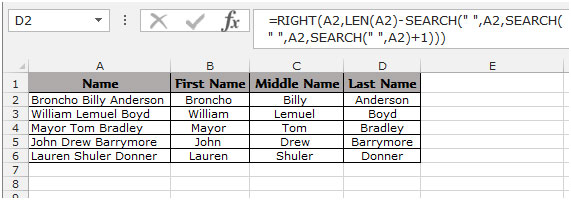
To pick the Last name from the list. We we will use the “RIGHT” function along with the “SEARCH” and “LEN” function.

• Select the Cell D2, write the formula =RIGHT(A2,LEN(A2)-SEARCH(» «,A2,SEARCH(» «,A2,SEARCH(» «,A2)+1))) It will return the last name from the cell A2.
• To Copy the formula in all cells press key “CTRL + C” and select the cell D3 to D6 and press key “CTRL + V” on your keyboard.

This is the way we can split names through formula in Microsoft Excel.

To know more find the below examples:-

Extract file name from a path

How to split a full address into 3 or more separate columns