
In this tutorial we will learn about Excel VBA function
1) What is Visual Basic in Excel?
2) How to use VBA in Excel?
3) How to create User defined function?
4) How to write Macro?
How to write VBA code
Excel provides the user with a large collection of ready-made functions, more than enough to satisfy the average user. Many more can be added by installing the various add-ins that are available. Most calculations can be achieved with what is provided, but it isn’t long before you find yourself wishing that there was a function that did a particular job, and you can’t find anything suitable in the list. You need a UDF. A UDF (User Defined Function) is simply a function that you create yourself with VBA. UDFs are often called «Custom Functions». A UDF can remain in a code module attached to a workbook, in which case it will always be available when that workbook is open. Alternatively you can create your own add-in containing one or more functions that you can install into Excel just like a commercial add-in. UDFs can be accessed by code modules too. Often UDFs are created by developers to work solely within the code of a VBA procedure and the user is never aware of their existence. Like any function, the UDF can be as simple or as complex as you want. Let’s start with an easy one…
A Function to Calculate the Area of a Rectangle
Yes, I know you could do this in your head! The concept is very simple so you can concentrate on the technique. Suppose you need a function to calculate the area of a rectangle. You look through Excel’s collection of functions, but there isn’t one suitable. This is the calculation to be done:
AREA = LENGTH x WIDTH
Open a new workbook and then open the Visual Basic Editor (Tools > Macro > Visual Basic Editor or ALT+F11).
You will need a module in which to write your function so choose Insert > Module. Into the empty module type: Function Area and press ENTER.The Visual Basic Editor completes the line for you and adds an End Function line as if you were creating a subroutine.So far it looks like this…
Function Area()

End Function
Place your cursor between the brackets after «Area». If you ever wondered what the brackets are for, you are about to find out! We are going to specify the «arguments» that our function will take (an argument is a piece of information needed to do the calculation). Type Length as double, Width as double and click in the empty line underneath. Note that as you type, a scroll box pops-up listing all the things appropriate to what you are typing.

This feature is called Auto List Members. If it doesn’t appear either it is switched off (turn it on at Tools > Options > Editor) or you might have made a typing error earlier. It is a very useful check on your syntax. Find the item you need and double-click it to insert it into your code. You can ignore it and just type if you want. Your code now looks like this…
Function Area(Length As Double, Width As Double)

End Function
Declaring the data type of the arguments is not obligatory but makes sense. You could have typed Length, Width and left it as that, but warning Excel what data type to expect helps your code run more quickly and picks up errors in input. The double data type refers to number (which can be very large) and allows fractions. Now for the calculation itself. In the empty line first press the TAB key to indent your code (making it easier to read) and type Area = Length * Width. Here’s the completed code…
Function Area(Length As Double, Width As Double)
    Area = Length * Width
End Function
You will notice another of the Visual Basic Editor’s help features pop up as you were typing, Auto Quick Info…

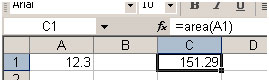
It isn’t relevant here. Its purpose is to help you write functions in VBA, by telling you what arguments are required. You can test your function right away. Switch to the Excel window and enter figures for Length and Width in separate cells. In a third cell enter your function as if it were one of the built-in ones. In this example cell A1 contains the length (17) and cell B1 the width (6.5). In C1 I typed =area(A1,B1) and the new function calculated the area (110.5)…

Sometimes, a function’s arguments can be optional. In this example we could make the Width argument optional. Supposing the rectangle happens to be a square with Length and Width equal. To save the user having to enter two arguments we could let them enter just the Length and have the function use that value twice (i.e. multiply Length x Length). So the function knows when it can do this we must include an IF Statement to help it decide. Change the code so that it looks like this…
Function Area(Length As Double, Optional Width As Variant)
    If IsMissing(Width) Then
        Area = Length * Length
    Else
        Area = Length * Width
    End If
End Function
Note that the data type for Width has been changed to Variant to allow for null values. The function now allows the user to enter just one argument e.g. =area(A1).The IF Statement in the function checks to see if the Width argument has been supplied and calculates accordingly…
A Function to Calculate Fuel Consumption
I like to keep a check on my car’s fuel consumption so when I buy fuel I make a note of the mileage and how much fuel it takes to fill the tank. Here in the UK fuel is sold in litres. The car’s milometer (OK, so it’s an odometer) records distance in miles. And because I’m too old and stupid to change, I only understand MPG (miles per gallon). Now if you think that’s all a bit sad, how about this. When I get home I open up Excel and enter the data into a worksheet that calculates the MPG for me and charts the car’s performance. The calculation is the number of miles the car has travelled since the last fill-up divided by the number of gallons of fuel used…
MPG = (MILES THIS FILL — MILES LAST FILL) / GALLONS OF FUEL
but because the fuel comes in litres and there are 4.546 litres in a gallon..
MPG = (MILES THIS FILL — MILES LAST FILL) / LITRES OF FUEL x 4.546
Here’s how I wrote the function…
Function MPG(StartMiles As Integer, FinishMiles As Integer, Litres As Single)
    MPG = (FinishMiles - StartMiles) / Litres * 4.546
End Function
and here’s how it looks on the worksheet…

Not all functions perform mathematical calculations. Here’s one that provides information…
A Function That Gives the Name of the Day
I am often asked if there is a date function that gives the day of the week as text (e.g. Monday). The answer is no*, but it’s quite easy to create one. (*Addendum: Did I say no? Check the note below to see the function I forgot!). Excel has the WEEKDAY function, which returns the day of the week as a number from 1 to 7. You get to choose which day is 1 if you don’t like the default (Sunday). In the example below the function returns «5» which I happen to know means «Thursday».

But I don’t want to see a number, I want to see «Thursday». I could modify the calculation by adding a VLOOKUP function that referred to a table somewhere containing a list of numbers and a corresponding list of day names. Or I could have the whole thing self-contained with multiple nested IF statements. Too complicated! The answer is a custom function…
Function DayName(InputDate As Date)
    Dim DayNumber As Integer
    DayNumber = Weekday(InputDate, vbSunday)
    Select Case DayNumber
        Case 1
            DayName = "Sunday"
        Case 2
            DayName = "Monday"
        Case 3
            DayName = "Tuesday"
        Case 4
            DayName = "Wednesday"
        Case 5
            DayName = "Thursday"
        Case 6
            DayName = "Friday"
        Case 7
            DayName = "Saturday"
    End Select
End Function
I’ve called my function «DayName» and it takes a single argument, which I call «InputDate» which (of course) has to be a date. Here’s how it works…
- The first line of the function declares a variable that I have called «DayNumber» which will be an Integer (i.e. a whole number).
- The next line of the function assigns a value to that variable using Excel’s WEEKDAY function. The value will be a number between 1 and 7. Although the default is 1=Sunday, I’ve included it anyway for clarity.
- Finally a Case Statement examines the value of the variable and returns the appropriate piece of text.
Here’s how it looks on the worksheet…

Accessing Your Custom Functions
If a workbook has a VBA code module attached to it that contains custom functions, those functions can be easily addressed within the same workbook as demonstrated in the examples above. You use the function name as if it were one of Excel’s built-in functions.
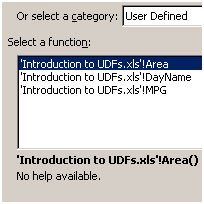
You can also find the functions listed in the Function Wizard (sometimes called the Paste Function tool). Use the wizard to insert a function in the normal way (Insert > Function).
Scroll down the list of function categories to find User Defined and select it to see a list of available UDFs…


You can see that the user defined functions lack any description other than the unhelpful «No help available» message, but you can add a short description…
Make sure you are in the workbook that contains the functions. Go to Tools > Macro > Macros. You won’t see your functions listed here but Excel knows about them! In the Macro Name box at the top of the dialog, type the name of the function, then click the dialog’s Options button. If the button is greyed out either you’ve spelled the function name wrong, or you are in the wrong workbook, or it doesn’t exist! This opens another dialog into which you can enter a short description of the function. Click OK to save the description and (here’s the confusing bit) click Cancel to close the Macro dialog box. Remember to Save the workbook containing the function. Next time you go to the Function Wizard your UDF will have a description…

Like macros, user defined functions can be used in any other workbook as long as the workbook containing them is open. However it is not good practice to do this. Entering the function in a different workbook is not simple. You have to add its host workbook’s name to the function name. This isn’t difficult if you rely on the Function Wizard, but clumsy to write out manually. The Function Wizard shows the full names of any UDFs in other workbooks…
If you open the workbook in which you used the function at a time when the workbook containing the function is closed, you will see an error message in the cell in which you used the function. Excel has forgotten about it! Open the function’s host workbook, recalculate, and all is fine again. Fortunately there is a better way.
If you want to write User Defined Functions for use in more than one workbook the best method is to create an Excel Add-In. Find out how to do this in the tutorial Build an Excel Add-In.
Addendum
I really ought to know better! Never, ever, say never! Having told you that there isn’t a function that provides the day’s name, I have now remembered the one that can. Look at this example…
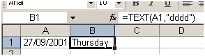
The TEXT function returns the value of a cell as text in a specific number format. So in the example I could have chosen =TEXT(A1,»ddd») to return «Thu», =TEXT(A1,»mmmm») to return «September» etc. The Excel’s help has some more examples of ways to use this function.
If you liked our blogs, share it with your friends on Facebook. And also you can follow us on Twitter and Facebook.
We would love to hear from you, do let us know how we can improve, complement or innovate our work and make it better for you. Write us at info@exceltip.com
ABS function
Math and trigonometry: Returns the absolute value of a number
ACCRINT function
Financial: Returns the accrued interest for a security that pays periodic interest
ACCRINTM function
Financial: Returns the accrued interest for a security that pays interest at maturity
ACOS function
Math and trigonometry: Returns the arccosine of a number
ACOSH function
Math and trigonometry: Returns the inverse hyperbolic cosine of a number
ACOT function

Math and trigonometry: Returns the arccotangent of a number
ACOTH function
Math and trigonometry: Returns the hyperbolic arccotangent of a number
AGGREGATE function
Math and trigonometry: Returns an aggregate in a list or database
ADDRESS function
Lookup and reference: Returns a reference as text to a single cell in a worksheet
AMORDEGRC function
Financial: Returns the depreciation for each accounting period by using a depreciation coefficient
AMORLINC function
Financial: Returns the depreciation for each accounting period
AND function
Logical: Returns TRUE if all of its arguments are TRUE
ARABIC function
Math and trigonometry: Converts a Roman number to Arabic, as a number
AREAS function
Lookup and reference: Returns the number of areas in a reference
ARRAYTOTEXT function

Text: Returns an array of text values from any specified range
ASC function
Text: Changes full-width (double-byte) English letters or katakana within a character string to half-width (single-byte) characters
ASIN function
Math and trigonometry: Returns the arcsine of a number
ASINH function
Math and trigonometry: Returns the inverse hyperbolic sine of a number
ATAN function
Math and trigonometry: Returns the arctangent of a number
ATAN2 function
Math and trigonometry: Returns the arctangent from x- and y-coordinates
ATANH function
Math and trigonometry: Returns the inverse hyperbolic tangent of a number
AVEDEV function
Statistical: Returns the average of the absolute deviations of data points from their mean
AVERAGE function
Statistical: Returns the average of its arguments
AVERAGEA function
Statistical: Returns the average of its arguments, including numbers, text, and logical values
AVERAGEIF function
Statistical: Returns the average (arithmetic mean) of all the cells in a range that meet a given criteria
AVERAGEIFS function
Statistical: Returns the average (arithmetic mean) of all cells that meet multiple criteria.
BAHTTEXT function
Text: Converts a number to text, using the ß (baht) currency format
BASE function
Math and trigonometry: Converts a number into a text representation with the given radix (base)
BESSELI function
Engineering: Returns the modified Bessel function In(x)
BESSELJ function
Engineering: Returns the Bessel function Jn(x)
BESSELK function
Engineering: Returns the modified Bessel function Kn(x)
BESSELY function
Engineering: Returns the Bessel function Yn(x)
BETADIST function
Compatibility: Returns the beta cumulative distribution function
In Excel 2007, this is a Statistical function.
BETA.DIST function

Statistical: Returns the beta cumulative distribution function
BETAINV function
Compatibility: Returns the inverse of the cumulative distribution function for a specified beta distribution
In Excel 2007, this is a Statistical function.
BETA.INV function
Statistical: Returns the inverse of the cumulative distribution function for a specified beta distribution
BIN2DEC function
Engineering: Converts a binary number to decimal
BIN2HEX function
Engineering: Converts a binary number to hexadecimal
BIN2OCT function
Engineering: Converts a binary number to octal
BINOMDIST function
Compatibility: Returns the individual term binomial distribution probability
In Excel 2007, this is a Statistical function.
BINOM.DIST function
Statistical: Returns the individual term binomial distribution probability
BINOM.DIST.RANGE function
Statistical: Returns the probability of a trial result using a binomial distribution
BINOM.INV function
Statistical: Returns the smallest value for which the cumulative binomial distribution is less than or equal to a criterion value
BITAND function
Engineering: Returns a ‘Bitwise And’ of two numbers
BITLSHIFT function
Engineering: Returns a value number shifted left by shift_amount bits
BITOR function
Engineering: Returns a bitwise OR of 2 numbers
BITRSHIFT function
Engineering: Returns a value number shifted right by shift_amount bits
BITXOR function
Engineering: Returns a bitwise ‘Exclusive Or’ of two numbers
BYCOL
Logical: Applies a LAMBDA to each column and returns an array of the results
BYROW
Logical: Applies a LAMBDA to each row and returns an array of the results
CALL function
Add-in and Automation: Calls a procedure in a dynamic link library or code resource
CEILING function
Compatibility: Rounds a number to the nearest integer or to the nearest multiple of significance
CEILING.MATH function
Math and trigonometry: Rounds a number up, to the nearest integer or to the nearest multiple of significance
CEILING.PRECISE function
Math and trigonometry: Rounds a number the nearest integer or to the nearest multiple of significance. Regardless of the sign of the number, the number is rounded up.
CELL function
Information: Returns information about the formatting, location, or contents of a cell
This function is not available in Excel for the web.
CHAR function
Text: Returns the character specified by the code number
CHIDIST function
Compatibility: Returns the one-tailed probability of the chi-squared distribution
Note: In Excel 2007, this is a Statistical function.
CHIINV function
Compatibility: Returns the inverse of the one-tailed probability of the chi-squared distribution
Note: In Excel 2007, this is a Statistical function.
CHITEST function
Compatibility: Returns the test for independence
Note: In Excel 2007, this is a Statistical function.
CHISQ.DIST function
Statistical: Returns the cumulative beta probability density function
CHISQ.DIST.RT function
Statistical: Returns the one-tailed probability of the chi-squared distribution
CHISQ.INV function
Statistical: Returns the cumulative beta probability density function
CHISQ.INV.RT function
Statistical: Returns the inverse of the one-tailed probability of the chi-squared distribution
CHISQ.TEST function
Statistical: Returns the test for independence
CHOOSE function
Lookup and reference: Chooses a value from a list of values
CHOOSECOLS
Lookup and reference: Returns the specified columns from an array
CHOOSEROWS
Lookup and reference: Returns the specified rows from an array
CLEAN function
Text: Removes all nonprintable characters from text
CODE function
Text: Returns a numeric code for the first character in a text string
COLUMN function
Lookup and reference: Returns the column number of a reference
COLUMNS function
Lookup and reference: Returns the number of columns in a reference
COMBIN function
Math and trigonometry: Returns the number of combinations for a given number of objects
COMBINA function
Math and trigonometry:
Returns the number of combinations with repetitions for a given number of items
COMPLEX function
Engineering: Converts real and imaginary coefficients into a complex number
CONCAT function

Text: Combines the text from multiple ranges and/or strings, but it doesn’t provide the delimiter or IgnoreEmpty arguments.
CONCATENATE function
Text: Joins several text items into one text item
CONFIDENCE function
Compatibility: Returns the confidence interval for a population mean
In Excel 2007, this is a Statistical function.
CONFIDENCE.NORM function
Statistical: Returns the confidence interval for a population mean
CONFIDENCE.T function
Statistical: Returns the confidence interval for a population mean, using a Student’s t distribution
CONVERT function
Engineering: Converts a number from one measurement system to another
CORREL function
Statistical: Returns the correlation coefficient between two data sets
COS function
Math and trigonometry: Returns the cosine of a number
COSH function
Math and trigonometry: Returns the hyperbolic cosine of a number
COT function
Math and trigonometry: Returns the hyperbolic cosine of a number
COTH function
Math and trigonometry: Returns the cotangent of an angle
COUNT function
Statistical: Counts how many numbers are in the list of arguments
COUNTA function
Statistical: Counts how many values are in the list of arguments
COUNTBLANK function
Statistical: Counts the number of blank cells within a range
COUNTIF function
Statistical: Counts the number of cells within a range that meet the given criteria
COUNTIFS function
Statistical: Counts the number of cells within a range that meet multiple criteria
COUPDAYBS function
Financial: Returns the number of days from the beginning of the coupon period to the settlement date
COUPDAYS function
Financial: Returns the number of days in the coupon period that contains the settlement date
COUPDAYSNC function
Financial: Returns the number of days from the settlement date to the next coupon date
COUPNCD function
Financial: Returns the next coupon date after the settlement date
COUPNUM function
Financial: Returns the number of coupons payable between the settlement date and maturity date
COUPPCD function
Financial: Returns the previous coupon date before the settlement date
COVAR function
Compatibility: Returns covariance, the average of the products of paired deviations
In Excel 2007, this is a Statistical function.
COVARIANCE.P function
Statistical: Returns covariance, the average of the products of paired deviations
COVARIANCE.S function
Statistical: Returns the sample covariance, the average of the products deviations for each data point pair in two data sets
CRITBINOM function
Compatibility: Returns the smallest value for which the cumulative binomial distribution is less than or equal to a criterion value
In Excel 2007, this is a Statistical function.
CSC function
Math and trigonometry: Returns the cosecant of an angle
CSCH function
Math and trigonometry: Returns the hyperbolic cosecant of an angle
CUBEKPIMEMBER function
Cube: Returns a key performance indicator (KPI) name, property, and measure, and displays the name and property in the cell. A KPI is a quantifiable measurement, such as monthly gross profit or quarterly employee turnover, used to monitor an organization’s performance.
CUBEMEMBER function
Cube: Returns a member or tuple in a cube hierarchy. Use to validate that the member or tuple exists in the cube.
CUBEMEMBERPROPERTY function
Cube: Returns the value of a member property in the cube. Use to validate that a member name exists within the cube and to return the specified property for this member.
CUBERANKEDMEMBER function
Cube: Returns the nth, or ranked, member in a set. Use to return one or more elements in a set, such as the top sales performer or top 10 students.
CUBESET function
Cube: Defines a calculated set of members or tuples by sending a set expression to the cube on the server, which creates the set, and then returns that set to Microsoft Office Excel.
CUBESETCOUNT function
Cube: Returns the number of items in a set.
CUBEVALUE function
Cube: Returns an aggregated value from a cube.
CUMIPMT function
Financial: Returns the cumulative interest paid between two periods
CUMPRINC function
Financial: Returns the cumulative principal paid on a loan between two periods
DATE function
Date and time: Returns the serial number of a particular date
DATEDIF function
Date and time: Calculates the number of days, months, or years between two dates. This function is useful in formulas where you need to calculate an age.
DATEVALUE function
Date and time: Converts a date in the form of text to a serial number
DAVERAGE function
Database: Returns the average of selected database entries
DAY function
Date and time: Converts a serial number to a day of the month
DAYS function
Date and time: Returns the number of days between two dates
DAYS360 function
Date and time: Calculates the number of days between two dates based on a 360-day year
DB function
Financial: Returns the depreciation of an asset for a specified period by using the fixed-declining balance method
DBCS function
Text: Changes half-width (single-byte) English letters or katakana within a character string to full-width (double-byte) characters
DCOUNT function
Database: Counts the cells that contain numbers in a database
DCOUNTA function
Database: Counts nonblank cells in a database
DDB function
Financial: Returns the depreciation of an asset for a specified period by using the double-declining balance method or some other method that you specify
DEC2BIN function
Engineering: Converts a decimal number to binary
DEC2HEX function
Engineering: Converts a decimal number to hexadecimal
DEC2OCT function
Engineering: Converts a decimal number to octal
DECIMAL function
Math and trigonometry: Converts a text representation of a number in a given base into a decimal number
DEGREES function
Math and trigonometry: Converts radians to degrees
DELTA function
Engineering: Tests whether two values are equal
DEVSQ function
Statistical: Returns the sum of squares of deviations
DGET function
Database: Extracts from a database a single record that matches the specified criteria
DISC function
Financial: Returns the discount rate for a security
DMAX function
Database: Returns the maximum value from selected database entries
DMIN function
Database: Returns the minimum value from selected database entries
DOLLAR function
Text: Converts a number to text, using the $ (dollar) currency format
DOLLARDE function
Financial: Converts a dollar price, expressed as a fraction, into a dollar price, expressed as a decimal number
DOLLARFR function
Financial: Converts a dollar price, expressed as a decimal number, into a dollar price, expressed as a fraction
DPRODUCT function
Database: Multiplies the values in a particular field of records that match the criteria in a database
DROP
Lookup and reference: Excludes a specified number of rows or columns from the start or end of an array
DSTDEV function
Database: Estimates the standard deviation based on a sample of selected database entries
DSTDEVP function
Database: Calculates the standard deviation based on the entire population of selected database entries
DSUM function
Database: Adds the numbers in the field column of records in the database that match the criteria
DURATION function
Financial: Returns the annual duration of a security with periodic interest payments
DVAR function
Database: Estimates variance based on a sample from selected database entries
DVARP function
Database: Calculates variance based on the entire population of selected database entries
EDATE function
Date and time: Returns the serial number of the date that is the indicated number of months before or after the start date
EFFECT function
Financial: Returns the effective annual interest rate
ENCODEURL function
Web: Returns a URL-encoded string
This function is not available in Excel for the web.
EOMONTH function
Date and time: Returns the serial number of the last day of the month before or after a specified number of months
ERF function
Engineering: Returns the error function
ERF.PRECISE function
Engineering: Returns the error function
ERFC function
Engineering: Returns the complementary error function
ERFC.PRECISE function
Engineering: Returns the complementary ERF function integrated between x and infinity
ERROR.TYPE function
Information: Returns a number corresponding to an error type
EUROCONVERT function
Add-in and Automation: Converts a number to euros, converts a number from euros to a euro member currency, or converts a number from one euro member currency to another by using the euro as an intermediary (triangulation).
EVEN function
Math and trigonometry: Rounds a number up to the nearest even integer
EXACT function
Text: Checks to see if two text values are identical
EXP function
Math and trigonometry: Returns e raised to the power of a given number
EXPAND
Lookup and reference: Expands or pads an array to specified row and column dimensions
EXPON.DIST function
Statistical: Returns the exponential distribution
EXPONDIST function
Compatibility: Returns the exponential distribution
In Excel 2007, this is a Statistical function.
FACT function
Math and trigonometry: Returns the factorial of a number
FACTDOUBLE function
Math and trigonometry: Returns the double factorial of a number
FALSE function
Logical: Returns the logical value FALSE
F.DIST function
Statistical: Returns the F probability distribution
FDIST function
Compatibility: Returns the F probability distribution
In Excel 2007, this is a Statistical function.
F.DIST.RT function
Statistical: Returns the F probability distribution
FILTER function
Lookup and reference: Filters a range of data based on criteria you define
FILTERXML function
Web: Returns specific data from the XML content by using the specified XPath
This function is not available in Excel for the web.
FIND, FINDB functions
Text: Finds one text value within another (case-sensitive)
F.INV function
Statistical: Returns the inverse of the F probability distribution
F.INV.RT function
Statistical: Returns the inverse of the F probability distribution
FINV function
Compatibility: Returns the inverse of the F probability distribution
In Excel 2007this is a Statistical function.
FISHER function
Statistical: Returns the Fisher transformation
FISHERINV function
Statistical: Returns the inverse of the Fisher transformation
FIXED function
Text: Formats a number as text with a fixed number of decimals
FLOOR function
Compatibility: Rounds a number down, toward zero
In Excel 2007 and Excel 2010, this is a Math and trigonometry function.
FLOOR.MATH function
Math and trigonometry: Rounds a number down, to the nearest integer or to the nearest multiple of significance
FLOOR.PRECISE function
Math and trigonometry: Rounds a number the nearest integer or to the nearest multiple of significance. Regardless of the sign of the number, the number is rounded up.
FORECAST function
Statistical: Returns a value along a linear trend
In Excel 2016, this function is replaced with FORECAST.LINEAR as part of the new Forecasting functions, but it’s still available for compatibility with earlier versions.
FORECAST.ETS function

Statistical: Returns a future value based on existing (historical) values by using the AAA version of the Exponential Smoothing (ETS) algorithm
FORECAST.ETS.CONFINT function
Statistical: Returns a confidence interval for the forecast value at the specified target date
FORECAST.ETS.SEASONALITY function
Statistical: Returns the length of the repetitive pattern Excel detects for the specified time series
FORECAST.ETS.STAT function
Statistical: Returns a statistical value as a result of time series forecasting
FORECAST.LINEAR function
Statistical: Returns a future value based on existing values
FORMULATEXT function
Lookup and reference: Returns the formula at the given reference as text
FREQUENCY function
Statistical: Returns a frequency distribution as a vertical array
F.TEST function
Statistical: Returns the result of an F-test
FTEST function
Compatibility: Returns the result of an F-test
In Excel 2007, this is a Statistical function.
FV function
Financial: Returns the future value of an investment
FVSCHEDULE function
Financial: Returns the future value of an initial principal after applying a series of compound interest rates
GAMMA function
Statistical: Returns the Gamma function value
GAMMA.DIST function
Statistical: Returns the gamma distribution
GAMMADIST function
Compatibility: Returns the gamma distribution
In Excel 2007, this is a Statistical function.
GAMMA.INV function
Statistical: Returns the inverse of the gamma cumulative distribution
GAMMAINV function
Compatibility: Returns the inverse of the gamma cumulative distribution
In Excel 2007, this is a Statistical function.
GAMMALN function
Statistical: Returns the natural logarithm of the gamma function, Γ(x)
GAMMALN.PRECISE function
Statistical: Returns the natural logarithm of the gamma function, Γ(x)
GAUSS function
Statistical: Returns 0.5 less than the standard normal cumulative distribution
GCD function
Math and trigonometry: Returns the greatest common divisor
GEOMEAN function
Statistical: Returns the geometric mean
GESTEP function
Engineering: Tests whether a number is greater than a threshold value
GETPIVOTDATA function
Lookup and reference: Returns data stored in a PivotTable report
GROWTH function
Statistical: Returns values along an exponential trend
HARMEAN function
Statistical: Returns the harmonic mean
HEX2BIN function
Engineering: Converts a hexadecimal number to binary
HEX2DEC function
Engineering: Converts a hexadecimal number to decimal
HEX2OCT function
Engineering: Converts a hexadecimal number to octal
HLOOKUP function
Lookup and reference: Looks in the top row of an array and returns the value of the indicated cell
HOUR function
Date and time: Converts a serial number to an hour
HSTACK
Lookup and reference: Appends arrays horizontally and in sequence to return a larger array
HYPERLINK function
Lookup and reference: Creates a shortcut or jump that opens a document stored on a network server, an intranet, or the Internet
HYPGEOM.DIST function
Statistical: Returns the hypergeometric distribution
HYPGEOMDIST function
Compatibility: Returns the hypergeometric distribution
In Excel 2007, this is a Statistical function.
IF function
Logical: Specifies a logical test to perform
IFERROR function
Logical: Returns a value you specify if a formula evaluates to an error; otherwise, returns the result of the formula
IFNA function
Logical: Returns the value you specify if the expression resolves to #N/A, otherwise returns the result of the expression
IFS function
Logical: Checks whether one or more conditions are met and returns a value that corresponds to the first TRUE condition.
IMABS function
Engineering: Returns the absolute value (modulus) of a complex number
IMAGINARY function
Engineering: Returns the imaginary coefficient of a complex number
IMARGUMENT function
Engineering: Returns the argument theta, an angle expressed in radians
IMCONJUGATE function
Engineering: Returns the complex conjugate of a complex number
IMCOS function
Engineering: Returns the cosine of a complex number
IMCOSH function
Engineering: Returns the hyperbolic cosine of a complex number
IMCOT function
Engineering: Returns the cotangent of a complex number
IMCSC function
Engineering: Returns the cosecant of a complex number
IMCSCH function
Engineering: Returns the hyperbolic cosecant of a complex number
IMDIV function
Engineering: Returns the quotient of two complex numbers
IMEXP function
Engineering: Returns the exponential of a complex number
IMLN function
Engineering: Returns the natural logarithm of a complex number
IMLOG10 function
Engineering: Returns the base-10 logarithm of a complex number
IMLOG2 function
Engineering: Returns the base-2 logarithm of a complex number
IMPOWER function
Engineering: Returns a complex number raised to an integer power
IMPRODUCT function
Engineering: Returns the product of complex numbers
IMREAL function
Engineering: Returns the real coefficient of a complex number
IMSEC function
Engineering: Returns the secant of a complex number
IMSECH function
Engineering: Returns the hyperbolic secant of a complex number
IMSIN function
Engineering: Returns the sine of a complex number
IMSINH function
Engineering: Returns the hyperbolic sine of a complex number
IMSQRT function
Engineering: Returns the square root of a complex number
IMSUB function
Engineering: Returns the difference between two complex numbers
IMSUM function
Engineering: Returns the sum of complex numbers
IMTAN function
Engineering: Returns the tangent of a complex number
INDEX function
Lookup and reference: Uses an index to choose a value from a reference or array
INDIRECT function
Lookup and reference: Returns a reference indicated by a text value
INFO function
Information: Returns information about the current operating environment
This function is not available in Excel for the web.
INT function
Math and trigonometry: Rounds a number down to the nearest integer
INTERCEPT function
Statistical: Returns the intercept of the linear regression line
INTRATE function
Financial: Returns the interest rate for a fully invested security
IPMT function
Financial: Returns the interest payment for an investment for a given period
IRR function
Financial: Returns the internal rate of return for a series of cash flows
ISBLANK function
Information: Returns TRUE if the value is blank
ISERR function
Information: Returns TRUE if the value is any error value except #N/A
ISERROR function
Information: Returns TRUE if the value is any error value
ISEVEN function
Information: Returns TRUE if the number is even
ISFORMULA function
Information: Returns TRUE if there is a reference to a cell that contains a formula
ISLOGICAL function
Information: Returns TRUE if the value is a logical value
ISNA function
Information: Returns TRUE if the value is the #N/A error value
ISNONTEXT function
Information: Returns TRUE if the value is not text
ISNUMBER function
Information: Returns TRUE if the value is a number
ISODD function
Information: Returns TRUE if the number is odd
ISOMITTED
Information: Checks whether the value in a LAMBDA is missing and returns TRUE or FALSE
ISREF function
Information: Returns TRUE if the value is a reference
ISTEXT function
Information: Returns TRUE if the value is text
ISO.CEILING function
Math and trigonometry: Returns a number that is rounded up to the nearest integer or to the nearest multiple of significance
ISOWEEKNUM function
Date and time: Returns the number of the ISO week number of the year for a given date
ISPMT function
Financial: Calculates the interest paid during a specific period of an investment
JIS function
Text: Changes half-width (single-byte) characters within a string to full-width (double-byte) characters
KURT function
Statistical: Returns the kurtosis of a data set
LAMBDA
Logical: Create custom, reusable functions and call them by a friendly name
LARGE function
Statistical: Returns the k-th largest value in a data set
LCM function
Math and trigonometry: Returns the least common multiple
LEFT, LEFTB functions
Text: Returns the leftmost characters from a text value
LEN, LENB functions
Text: Returns the number of characters in a text string
LET
Logical: Assigns names to calculation results
LINEST function
Statistical: Returns the parameters of a linear trend
LN function
Math and trigonometry: Returns the natural logarithm of a number
LOG function
Math and trigonometry: Returns the logarithm of a number to a specified base
LOG10 function
Math and trigonometry: Returns the base-10 logarithm of a number
LOGEST function
Statistical: Returns the parameters of an exponential trend
LOGINV function
Compatibility: Returns the inverse of the lognormal cumulative distribution
LOGNORM.DIST function
Statistical: Returns the cumulative lognormal distribution
LOGNORMDIST function
Compatibility: Returns the cumulative lognormal distribution
LOGNORM.INV function
Statistical: Returns the inverse of the lognormal cumulative distribution
LOOKUP function
Lookup and reference: Looks up values in a vector or array
LOWER function
Text: Converts text to lowercase
MAKEARRAY
Logical: Returns a calculated array of a specified row and column size, by applying a LAMBDA
MAP
Logical: Returns an array formed by mapping each value in the array(s) to a new value by applying a LAMBDA to create a new value
MATCH function
Lookup and reference: Looks up values in a reference or array
MAX function
Statistical: Returns the maximum value in a list of arguments
MAXA function
Statistical: Returns the maximum value in a list of arguments, including numbers, text, and logical values
MAXIFS function
Statistical: Returns the maximum value among cells specified by a given set of conditions or criteria
MDETERM function
Math and trigonometry: Returns the matrix determinant of an array
MDURATION function
Financial: Returns the Macauley modified duration for a security with an assumed par value of $100
MEDIAN function
Statistical: Returns the median of the given numbers
MID, MIDB functions
Text: Returns a specific number of characters from a text string starting at the position you specify
MIN function
Statistical: Returns the minimum value in a list of arguments
MINIFS function
Statistical: Returns the minimum value among cells specified by a given set of conditions or criteria.
MINA function
Statistical: Returns the smallest value in a list of arguments, including numbers, text, and logical values
MINUTE function
Date and time: Converts a serial number to a minute
MINVERSE function
Math and trigonometry: Returns the matrix inverse of an array
MIRR function
Financial: Returns the internal rate of return where positive and negative cash flows are financed at different rates
MMULT function
Math and trigonometry: Returns the matrix product of two arrays
MOD function
Math and trigonometry: Returns the remainder from division
MODE function
Compatibility: Returns the most common value in a data set
In Excel 2007, this is a Statistical function.
MODE.MULT function
Statistical: Returns a vertical array of the most frequently occurring, or repetitive values in an array or range of data
MODE.SNGL function
Statistical: Returns the most common value in a data set
MONTH function
Date and time: Converts a serial number to a month
MROUND function
Math and trigonometry: Returns a number rounded to the desired multiple
MULTINOMIAL function
Math and trigonometry: Returns the multinomial of a set of numbers
MUNIT function
Math and trigonometry: Returns the unit matrix or the specified dimension
N function
Information: Returns a value converted to a number
NA function
Information: Returns the error value #N/A
NEGBINOM.DIST function
Statistical: Returns the negative binomial distribution
NEGBINOMDIST function
Compatibility: Returns the negative binomial distribution
In Excel 2007, this is a Statistical function.
NETWORKDAYS function
Date and time: Returns the number of whole workdays between two dates
NETWORKDAYS.INTL function
Date and time: Returns the number of whole workdays between two dates using parameters to indicate which and how many days are weekend days
NOMINAL function
Financial: Returns the annual nominal interest rate
NORM.DIST function
Statistical: Returns the normal cumulative distribution
NORMDIST function
Compatibility: Returns the normal cumulative distribution
In Excel 2007, this is a Statistical function.
NORMINV function
Statistical: Returns the inverse of the normal cumulative distribution
NORM.INV function
Compatibility: Returns the inverse of the normal cumulative distribution
Note: In Excel 2007, this is a Statistical function.
NORM.S.DIST function
Statistical: Returns the standard normal cumulative distribution
NORMSDIST function
Compatibility: Returns the standard normal cumulative distribution
In Excel 2007, this is a Statistical function.
NORM.S.INV function
Statistical: Returns the inverse of the standard normal cumulative distribution
NORMSINV function
Compatibility: Returns the inverse of the standard normal cumulative distribution
In Excel 2007, this is a Statistical function.
NOT function
Logical: Reverses the logic of its argument
NOW function
Date and time: Returns the serial number of the current date and time
NPER function
Financial: Returns the number of periods for an investment
NPV function
Financial: Returns the net present value of an investment based on a series of periodic cash flows and a discount rate
NUMBERVALUE function
Text: Converts text to number in a locale-independent manner
OCT2BIN function
Engineering: Converts an octal number to binary
OCT2DEC function
Engineering: Converts an octal number to decimal
OCT2HEX function
Engineering: Converts an octal number to hexadecimal
ODD function
Math and trigonometry: Rounds a number up to the nearest odd integer
ODDFPRICE function
Financial: Returns the price per $100 face value of a security with an odd first period
ODDFYIELD function
Financial: Returns the yield of a security with an odd first period
ODDLPRICE function
Financial: Returns the price per $100 face value of a security with an odd last period
ODDLYIELD function
Financial: Returns the yield of a security with an odd last period
OFFSET function
Lookup and reference: Returns a reference offset from a given reference
OR function
Logical: Returns TRUE if any argument is TRUE
PDURATION function
Financial: Returns the number of periods required by an investment to reach a specified value
PEARSON function
Statistical: Returns the Pearson product moment correlation coefficient
PERCENTILE.EXC function
Statistical: Returns the k-th percentile of values in a range, where k is in the range 0..1, exclusive
PERCENTILE.INC function
Statistical: Returns the k-th percentile of values in a range
PERCENTILE function
Compatibility: Returns the k-th percentile of values in a range
In Excel 2007, this is a Statistical function.
PERCENTRANK.EXC function
Statistical: Returns the rank of a value in a data set as a percentage (0..1, exclusive) of the data set
PERCENTRANK.INC function
Statistical: Returns the percentage rank of a value in a data set
PERCENTRANK function
Compatibility: Returns the percentage rank of a value in a data set
In Excel 2007, this is a Statistical function.
PERMUT function
Statistical: Returns the number of permutations for a given number of objects
PERMUTATIONA function
Statistical: Returns the number of permutations for a given number of objects (with repetitions) that can be selected from the total objects
PHI function
Statistical: Returns the value of the density function for a standard normal distribution
PHONETIC function
Text: Extracts the phonetic (furigana) characters from a text string
PI function
Math and trigonometry: Returns the value of pi
PMT function
Financial: Returns the periodic payment for an annuity
POISSON.DIST function
Statistical: Returns the Poisson distribution
POISSON function
Compatibility: Returns the Poisson distribution
In Excel 2007, this is a Statistical function.
POWER function
Math and trigonometry: Returns the result of a number raised to a power
PPMT function
Financial: Returns the payment on the principal for an investment for a given period
PRICE function
Financial: Returns the price per $100 face value of a security that pays periodic interest
PRICEDISC function
Financial: Returns the price per $100 face value of a discounted security
PRICEMAT function
Financial: Returns the price per $100 face value of a security that pays interest at maturity
PROB function
Statistical: Returns the probability that values in a range are between two limits
PRODUCT function
Math and trigonometry: Multiplies its arguments
PROPER function
Text: Capitalizes the first letter in each word of a text value
PV function
Financial: Returns the present value of an investment
QUARTILE function
Compatibility: Returns the quartile of a data set
In Excel 2007, this is a Statistical function.
QUARTILE.EXC function
Statistical: Returns the quartile of the data set, based on percentile values from 0..1, exclusive
QUARTILE.INC function
Statistical: Returns the quartile of a data set
QUOTIENT function
Math and trigonometry: Returns the integer portion of a division
RADIANS function
Math and trigonometry: Converts degrees to radians
RAND function
Math and trigonometry: Returns a random number between 0 and 1
RANDARRAY function
Math and trigonometry: Returns an array of random numbers between 0 and 1. However, you can specify the number of rows and columns to fill, minimum and maximum values, and whether to return whole numbers or decimal values.
RANDBETWEEN function
Math and trigonometry: Returns a random number between the numbers you specify
RANK.AVG function
Statistical: Returns the rank of a number in a list of numbers
RANK.EQ function
Statistical: Returns the rank of a number in a list of numbers
RANK function
Compatibility: Returns the rank of a number in a list of numbers
In Excel 2007, this is a Statistical function.
RATE function
Financial: Returns the interest rate per period of an annuity
RECEIVED function
Financial: Returns the amount received at maturity for a fully invested security
REDUCE
Logical: Reduces an array to an accumulated value by applying a LAMBDA to each value and returning the total value in the accumulator
REGISTER.ID function
Add-in and Automation: Returns the register ID of the specified dynamic link library (DLL) or code resource that has been previously registered
REPLACE, REPLACEB functions
Text: Replaces characters within text
REPT function
Text: Repeats text a given number of times
RIGHT, RIGHTB functions
Text: Returns the rightmost characters from a text value
ROMAN function
Math and trigonometry: Converts an arabic numeral to roman, as text
ROUND function
Math and trigonometry: Rounds a number to a specified number of digits
ROUNDDOWN function
Math and trigonometry: Rounds a number down, toward zero
ROUNDUP function
Math and trigonometry: Rounds a number up, away from zero
ROW function
Lookup and reference: Returns the row number of a reference
ROWS function
Lookup and reference: Returns the number of rows in a reference
RRI function
Financial: Returns an equivalent interest rate for the growth of an investment
RSQ function
Statistical: Returns the square of the Pearson product moment correlation coefficient
RTD function
Lookup and reference: Retrieves real-time data from a program that supports COM automation
SCAN
Logical: Scans an array by applying a LAMBDA to each value and returns an array that has each intermediate value
SEARCH, SEARCHB functions
Text: Finds one text value within another (not case-sensitive)
SEC function
Math and trigonometry: Returns the secant of an angle
SECH function
Math and trigonometry: Returns the hyperbolic secant of an angle
SECOND function
Date and time: Converts a serial number to a second
SEQUENCE function
Math and trigonometry: Generates a list of sequential numbers in an array, such as 1, 2, 3, 4
SERIESSUM function
Math and trigonometry: Returns the sum of a power series based on the formula
SHEET function
Information: Returns the sheet number of the referenced sheet
SHEETS function
Information: Returns the number of sheets in a reference
SIGN function
Math and trigonometry: Returns the sign of a number
SIN function
Math and trigonometry: Returns the sine of the given angle
SINH function
Math and trigonometry: Returns the hyperbolic sine of a number
SKEW function
Statistical: Returns the skewness of a distribution
SKEW.P function
Statistical: Returns the skewness of a distribution based on a population: a characterization of the degree of asymmetry of a distribution around its mean
SLN function
Financial: Returns the straight-line depreciation of an asset for one period
SLOPE function
Statistical: Returns the slope of the linear regression line
SMALL function
Statistical: Returns the k-th smallest value in a data set
SORT function
Lookup and reference: Sorts the contents of a range or array
SORTBY function
Lookup and reference: Sorts the contents of a range or array based on the values in a corresponding range or array
SQRT function
Math and trigonometry: Returns a positive square root
SQRTPI function
Math and trigonometry: Returns the square root of (number * pi)
STANDARDIZE function
Statistical: Returns a normalized value
STOCKHISTORY function
Financial: Retrieves historical data about a financial instrument
STDEV function
Compatibility: Estimates standard deviation based on a sample
STDEV.P function
Statistical: Calculates standard deviation based on the entire population
STDEV.S function
Statistical: Estimates standard deviation based on a sample
STDEVA function
Statistical: Estimates standard deviation based on a sample, including numbers, text, and logical values
STDEVP function
Compatibility: Calculates standard deviation based on the entire population
In Excel 2007, this is a Statistical function.
STDEVPA function
Statistical: Calculates standard deviation based on the entire population, including numbers, text, and logical values
STEYX function
Statistical: Returns the standard error of the predicted y-value for each x in the regression
SUBSTITUTE function
Text: Substitutes new text for old text in a text string
SUBTOTAL function
Math and trigonometry: Returns a subtotal in a list or database
SUM function
Math and trigonometry: Adds its arguments
SUMIF function
Math and trigonometry: Adds the cells specified by a given criteria
SUMIFS function
Math and trigonometry: Adds the cells in a range that meet multiple criteria
SUMPRODUCT function
Math and trigonometry: Returns the sum of the products of corresponding array components
SUMSQ function
Math and trigonometry: Returns the sum of the squares of the arguments
SUMX2MY2 function
Math and trigonometry: Returns the sum of the difference of squares of corresponding values in two arrays
SUMX2PY2 function
Math and trigonometry: Returns the sum of the sum of squares of corresponding values in two arrays
SUMXMY2 function
Math and trigonometry: Returns the sum of squares of differences of corresponding values in two arrays
SWITCH function
Logical: Evaluates an expression against a list of values and returns the result corresponding to the first matching value. If there is no match, an optional default value may be returned.
SYD function
Financial: Returns the sum-of-years’ digits depreciation of an asset for a specified period
T function
Text: Converts its arguments to text
TAN function
Math and trigonometry: Returns the tangent of a number
TANH function
Math and trigonometry: Returns the hyperbolic tangent of a number
TAKE
Lookup and reference: Returns a specified number of contiguous rows or columns from the start or end of an array
TBILLEQ function
Financial: Returns the bond-equivalent yield for a Treasury bill
TBILLPRICE function
Financial: Returns the price per $100 face value for a Treasury bill
TBILLYIELD function
Financial: Returns the yield for a Treasury bill
T.DIST function
Statistical: Returns the Percentage Points (probability) for the Student t-distribution
T.DIST.2T function
Statistical: Returns the Percentage Points (probability) for the Student t-distribution
T.DIST.RT function
Statistical: Returns the Student’s t-distribution
TDIST function
Compatibility: Returns the Student’s t-distribution
TEXT function
Text: Formats a number and converts it to text
TEXTAFTER
Text: Returns text that occurs after given character or string
TEXTBEFORE
Text: Returns text that occurs before a given character or string
TEXTJOIN
Text: Combines the text from multiple ranges and/or strings
TEXTSPLIT
Text: Splits text strings by using column and row delimiters
TIME function
Date and time: Returns the serial number of a particular time
TIMEVALUE function
Date and time: Converts a time in the form of text to a serial number
T.INV function
Statistical: Returns the t-value of the Student’s t-distribution as a function of the probability and the degrees of freedom
T.INV.2T function
Statistical: Returns the inverse of the Student’s t-distribution
TINV function
Compatibility: Returns the inverse of the Student’s t-distribution
TOCOL
Lookup and reference: Returns the array in a single column
TOROW
Lookup and reference: Returns the array in a single row
TODAY function
Date and time: Returns the serial number of today’s date
TRANSPOSE function
Lookup and reference: Returns the transpose of an array
TREND function
Statistical: Returns values along a linear trend
TRIM function
Text: Removes spaces from text
TRIMMEAN function
Statistical: Returns the mean of the interior of a data set
TRUE function
Logical: Returns the logical value TRUE
TRUNC function
Math and trigonometry: Truncates a number to an integer
T.TEST function
Statistical: Returns the probability associated with a Student’s t-test
TTEST function
Compatibility: Returns the probability associated with a Student’s t-test
In Excel 2007, this is a Statistical function.
TYPE function
Information: Returns a number indicating the data type of a value
UNICHAR function
Text: Returns the Unicode character that is references by the given numeric value
UNICODE function
Text: Returns the number (code point) that corresponds to the first character of the text
UNIQUE function
Lookup and reference: Returns a list of unique values in a list or range
UPPER function
Text: Converts text to uppercase
VALUE function
Text: Converts a text argument to a number
VALUETOTEXT
Text: Returns text from any specified value
VAR function
Compatibility: Estimates variance based on a sample
In Excel 2007, this is a Statistical function.
VAR.P function
Statistical: Calculates variance based on the entire population
VAR.S function
Statistical: Estimates variance based on a sample
VARA function
Statistical: Estimates variance based on a sample, including numbers, text, and logical values
VARP function
Compatibility: Calculates variance based on the entire population
In Excel 2007, this is a Statistical function.
VARPA function
Statistical: Calculates variance based on the entire population, including numbers, text, and logical values
VDB function
Financial: Returns the depreciation of an asset for a specified or partial period by using a declining balance method
VLOOKUP function
Lookup and reference: Looks in the first column of an array and moves across the row to return the value of a cell
VSTACK
Look and reference: Appends arrays vertically and in sequence to return a larger array
WEBSERVICE function
Web: Returns data from a web service.
This function is not available in Excel for the web.
WEEKDAY function
Date and time: Converts a serial number to a day of the week
WEEKNUM function
Date and time: Converts a serial number to a number representing where the week falls numerically with a year
WEIBULL function
Compatibility: Calculates variance based on the entire population, including numbers, text, and logical values
In Excel 2007, this is a Statistical function.
WEIBULL.DIST function
Statistical: Returns the Weibull distribution
WORKDAY function
Date and time: Returns the serial number of the date before or after a specified number of workdays
WORKDAY.INTL function
Date and time: Returns the serial number of the date before or after a specified number of workdays using parameters to indicate which and how many days are weekend days
WRAPCOLS
Look and reference: Wraps the provided row or column of values by columns after a specified number of elements
WRAPROWS
Look and reference: Wraps the provided row or column of values by rows after a specified number of elements
XIRR function
Financial: Returns the internal rate of return for a schedule of cash flows that is not necessarily periodic
XLOOKUP function
Lookup and reference: Searches a range or an array, and returns an item corresponding to the first match it finds. If a match doesn’t exist, then XLOOKUP can return the closest (approximate) match.
XMATCH function
Lookup and reference: Returns the relative position of an item in an array or range of cells.
XNPV function
Financial: Returns the net present value for a schedule of cash flows that is not necessarily periodic
XOR function
Logical: Returns a logical exclusive OR of all arguments
YEAR function
Date and time: Converts a serial number to a year
YEARFRAC function
Date and time: Returns the year fraction representing the number of whole days between start_date and end_date
YIELD function
Financial: Returns the yield on a security that pays periodic interest
YIELDDISC function
Financial: Returns the annual yield for a discounted security; for example, a Treasury bill
YIELDMAT function
Financial: Returns the annual yield of a security that pays interest at maturity
Z.TEST function
Statistical: Returns the one-tailed probability-value of a z-test
ZTEST function
Compatibility: Returns the one-tailed probability-value of a z-test
In Excel 2007, this is a Statistical function.
15 Most Common Excel Functions You Must Know + How to Use Them
Microsoft Excel is one of the most well-known computer applications. It has changed the way people and companies work with data.
Thus, learning Excel can help with both your career and your personal needs.
Excel runs using functions and there are roughly 500 of them! These range from basic arithmetic to complex statistics.

If you’re a new Excel user, this sheer quantity can be quite daunting.
So we are here to help you! 🤝
We have rounded up 15 of the most common and useful Excel functions that you need to learn. We also prepared a practice workbook for you to follow along with the examples. Download it here.
Let’s get started!
What are Excel functions?
Excel is used to calculate and manipulate numbers and text. To do this, you use formulas!
Formulas are expressions that tell Excel what you want to do with the data. They begin with the equal symbol (=) followed by a combination of operators and functions.
What are operators?
These are symbols that specify the type of calculation you want to perform on the elements of a formula.
For example, to add two numbers, you can type “=1+1” into a cell. Once you hit Enter, Excel will run the formula and return the result which is 2.
Here are some examples of common operators:

Excel automatically treats cell contents that start with (=) as formulas. This also applies when you begin a cell with the plus (+) or minus (-) symbols.
You can bypass this by adding a leading apostrophe (‘). This is how you can show formulas as text like in the table above.
Order of operation and using parentheses in Excel formulas
Generally, Excel follows PEMDAS when calculating formulas. PEMDAS means parentheses first, then exponents, then multiplication and division, then addition and subtraction.

What are functions?
These are predefined processes in Excel. Each function in Excel has a unique name and specific input(s). The function takes these inputs and performs the corresponding calculation.
The inputs or arguments of an Excel function are always enclosed in parentheses.
For example, this is the syntax for the MAX function:
=MAX(number1, [number2], …)
The list of numbers where you want to find the maximum value is placed inside the parentheses.

Using a cell or a range as input
As you learn more about Excel, you’ll find that Excel formulas rarely consist of individual numbers only like in the formula “=1+1”.

Thus, referencing cells is important in Excel and you can learn more by clicking here.
Alright! You’ve just learned how a function in Excel works.
Let’s dive right into the list! 🤿
We will start with basic Excel functions and then move on to more advanced functions.
Basic Math Functions (Beginner Level ★☆☆)
1. SUM
This is the first function in Excel that most new users need. As the name implies, the SUM function adds up all the values in a specified group of cells or range.
Syntax: =SUM(number1, [number2], …)
Try it out in the practice workbook.

If you want to get the total quiz score for each student, you can use the SUM function. In this case, the input range will be all four quiz scores for each student.
1. Type this formula into cell F2:
=SUM(B2:E2)
You can also type “=SUM(B2,C2,D2,E2)” but “=SUM(B2:E2)” is much simpler.

2. Press Enter. Excel then evaluates the formula and the cell returns the number for the total which is 360.
3. Copy this for the rest of the students or drag down the fill handle.

Notice that the SUM function ignores the cells containing text. (“X” meaning the student was unable to take the quiz)
Most of the basic math functions in Excel ignore non-numeric values such as text, date, and time.
2. COUNT
Next up is the COUNT function. It returns the number of cells containing numeric values within the input range.
Syntax: =COUNT(value1, [value2], …)
1. To get the number of quizzes taken by each student, use this formula in cell G2:
=COUNT(B2:E2)
2. Hit Enter and fill in the rows below.

If you would like to include non-numeric values in the count, you can use the COUNTA function. To count the number of blank cells, you can use the COUNTBLANK function.
Learn more about the COUNT function and its variants here.
3. AVERAGE
The average of a list of numbers is just the total divided by how many numbers there are in that list.
This is easy enough to calculate the quiz scores. You already have the SUM and the COUNT of quizzes for each student.
But, it gets even easier using the AVERAGE function in Excel.
Syntax: =AVERAGE (value1, [value2], …)
1. Type this into cell H2:
=AVERAGE(B2:E2)
2. Hit Enter and fill in the rows below.


Logical Functions (Intermediate Level – ★★☆)
Let’s raise the difficulty level a little bit.
A logical function in Excel allows you to make comparisons and use the results to change how a formula calculates.
4. IF
The IF function is a very popular function in Excel and it is actually quite easy to learn.
Syntax: =IF(logical_test, value_if_true, [value_if_false])
This function checks if a logical test is either TRUE or FALSE. It then returns the specified value based on the result.

Using the average score of each student, try to assign PASS or FAIL grades. Assume that the passing score for this class is 60.
1. Begin the formula in cell C2 with “=IF(“
The logical_test is to check if the average score in Column B is greater than or equal to (>=) the passing score of 60.
2. So, the formula becomes:
=IF(B2>=60,
If the comparison returns TRUE, then the formula should return the text “PASS”. Thus, the value_if_true argument should be “PASS”.
And if it returns FALSE, then the value_if_false argument should be “FAIL”.
3. Thus, the formula becomes:
=IF(B2>=60,”PASS”,”FAIL”)
4. Hit Enter and fill in the rows below.

What if you needed to assign grades according to a scale instead of just “PASS” and “FAIL”?
For that, you have to use multiple criteria or logical tests. While this is possible using nested IF functions, it can get messy very quickly. Instead, you can use the IFS function.
5. IFS function
The IFS function was introduced in Excel 2016 to replace nested IF functions.
This function works by evaluating the first logical test or criteria. It returns the corresponding value if it is TRUE. But if it is FALSE, the function proceeds to evaluate the second criteria, and so on.
📖 In other words, the IFS function outputs the value that corresponds to the first specified criteria that is true.
Syntax: =IFS(logical_test1, value_if_true1, [logical_test2], [value_if_true2],..)

1. First, the formula should check if the average score (column B) is above or equal to 90. If yes, it should return “A”.
=IFS(B2>=90,”A”,
2. If not, it should then check if the average score is greater than or equal to 80. If yes, it should return “B”. If you do this up to grade D, the formula becomes:
=IFS(B2>=90,”A”,B2>=80,”B”,B2>=70,”C”,B2>=60,”D”,
3. For the last grade “F”, put “TRUE” for the logical test.
The IFS function will only evaluate the last specified criteria if all of the previous logical values were FALSE. Thus, you can set the last criteria to always be TRUE thus making it a “catch all” statement.
The final formula is then:
=IFS(B2>=90,”A”,B2>=80,”B”,B2>=70,”C”,B2>=60,”D”,TRUE,”F”)

PRO-TIP:
You can use absolute cell references and a reference table when working with long formulas.
That way, you don’t have to revisit all of the arguments in the formula if you need to change some values.
For example, using the table and formula shown below, you can easily change the grading scale in use.
=IFS(B2>=$H$2,$F$2,B2>=$H$3,$F$3,B2>
=$H$4,$F$4,B2>=$H$5,$F$5,TRUE,$F$6)

Text Functions (Intermediate Level – ★★☆)
In this next section, you will see how Excel can also be used to manipulate text.
In the “Class List” worksheet of the practice workbook, the full name of each student is listed in Column A. Your goal is to rearrange these from “first name last name” to “last name_first name” in Column F.

To do this, you first have to extract the first name and the last name from Column A.
6. FIND
The names are separated by a space character ” “. So, you have to identify the position of the space within each text string in Column A.
The FIND function in Excel returns the number or position of a specified character or substring within another text string.
Syntax: =FIND(find_text, within_text, [start_num])
To get the position of the space ” “, type this formula:
=FIND(” “,A2)

Next, take a look at the LEN function.
7. LEN
This function returns the number of characters in a text string.
Syntax: =LEN(text)
To get the number of characters in each student’s name:
=LEN(A2)

Now you can move on to extracting the first and last name using the MID function in Excel.
8. MID
This function extracts a given number of characters from the middle of a text string.
Syntax: = MID(text, start_num, num_chars)
It is one of three text functions that are used to extract text. The other two are LEFT and RIGHT which extract text from the start and end of a text string respectively.
The first name starts at the very first character of the text string. So, you extract starting from position 1. Then the length of the first name is given by the position of the space character minus 1.
So, the formula to extract the first name or first word from a text string is:
=MID(A2,1,B2-1)
Or, you can express it directly using the FIND formula earlier.
=MID(A2,1,FIND(” “,A2)-1)

For the last name, you can extract it starting from the position of the space character plus 1. Its length is just the length of the entire text string minus the position of the space character.
=MID(A2,B2+1,C2-B2)
Or, using the FIND and LEN formulas earlier:
=MID(A2,FIND(” “,A2)+1,LEN(A2)-FIND(” “,A2))

Now you can combine the last name and the first name in the desired order using the CONCAT function.
9. CONCAT
Like IFS, CONCAT is another newly introduced function in Excel 2016. It replaced the old CONCATENATE function.
Syntax: =CONCAT(text1, [text2],…)
Combine the last name and the first name with a comma and space character “, ” in between.
=CONCAT(E2,”, “,D2)

PRO-TIP:
In the above example, you used helper columns for FIND, LEN, and MID to help build the final formula and visualize how it works.
In real-world applications, you can use a single long formula to get the results like this:
=CONCAT(MID(A2,FIND(” “,A2)+1,LEN(A2)
-FIND(” “,A2)),”, “,MID(A2,1,FIND(” “,A2)-1))

Lookup and Reference Functions (Advanced Level – ★★★)
In this final section, we will focus on functions that allow you to look for specific data points and refer to them.
Take a look at the “Schedule” worksheet.

10. COLUMN
The COLUMN function in Excel returns the column number of a given cell.
Syntax: =COLUMN([reference])
Let’s try to assign specific dates for each quiz. For example, you may want the quizzes to be held every Monday. This means that the first quiz date should be offset by 1 week or 7 days for each succeeding quiz date.
You can use the column number to multiply the 7 days offset for each week like this:
=$B$2+(COLUMN()-2)*7

Two (2) is subtracted from the column number so that the sequence starts at 1.
You can also get this result using the much simpler “=B2+7” since you are only adding a fixed number of days to each date. 🤔
But, using the COLUMN function, you can create complex patterns.
Take this pattern for example:
The quizzes are still held every Monday. But every third week, they are held on Wednesday instead.
Here is the formula for this pattern:
=$B$2+(COLUMN()-2)*7+IF(MOD(COLUMN()-1,3)=0,2,0)


The MOD function in Excel returns the remainder after a number is divided by a given divisor. It’s part of the Math & Trig group of functions.
This group includes other fun functions such as ABS which returns the absolute value of a number and ROUND which rounds a number to a specified number of digits.
Learn more about the function groups towards the end of this article!
11. ROW
Next, take a look at the ROW function. It works exactly like COLUMN but it returns the row number instead.
Syntax: =ROW([reference])
In this next example, you will assign the seating plans. You can try different seating arrangements using the ROW function.
Assume R1C1 is the seat closest to the teacher’s desk.
1. You can have the students seated one seat after another and in two columns:
=CONCAT(“R”,MOD(ROW()-6,3)*2+1,”C”,INT((ROW()-6)/3)*2+1)

2. Or they can sit in rows of 3 and columns of 2
=CONCAT(“R”,MOD(ROW()-6,2)*2+1,”C”,INT((ROW()-6)/2)*2+1)

3. You can also sit them in the farthest rows:
=CONCAT(“R”,MOD(ROW()-6,2)*4+1,”C”,INT((ROW()-6)/2)*2+1)

4. Or in the farthest columns:
=CONCAT(“R”,MOD(ROW()-6,3)*2+1,”C”,INT((ROW()-6)/3)*4+1)

Manually creating seating patterns for small sets like this one is easy. But a formula like those shown above definitely helps especially for larger sets like 50, 100, or even more.
The COLUMN and ROW functions are rarely used on their own. Like IF and IFS, you use them with other functions to change how the formula is calculated.
12. MATCH
Now, open up the “Lookup” worksheet.
In the next few examples, you will create a search feature that allows students to look up their names. They can then see their scores from past quizzes and their assigned seats for the next quizzes.
To start, you will use the MATCH function. It searches for a specified item within a given range of cells. It then returns the relative position of the first match.
Syntax: =MATCH(lookup_value, lookup_array, [match_type])
- The lookup_value is the item you want to search for. So, set this to cell B2.
- The lookup_array is the range or table array where you want to search. Use F2:F7 from the “Class List” worksheet.
- For the match_type, set this to zero so that the function searches for an exact match. (Learn more about MATCH and the different match types in this article)
The formula then becomes:
=MATCH(B2,’Class List’!F2:F7,0)

However, it only works correctly if the name is entered exactly as it is written in Column F of the Class List.
To fix this, you can use the asterisk “*” wildcard character so that searching for either first or last name works.
You can also enclose the formula in an IFNA function. This way, if the formula cannot find the given name in the table, it will return a phrase like “No result found”.


13. INDEX
The INDEX function retrieves a value from a given table array based on the provided row and column numbers.
Syntax: =INDEX (array, row_num, [col_num])
Similar to the MATCH example, you need to specify where the range or array lookup is.

For row_num, you can use the earlier MATCH result at Cell B5. Then for col_num, use 1 for the First Name:
=INDEX(‘Class List’!D2:E7,B5,1)

And set col_num to 2 for the Last Name.
=INDEX(‘Class List’!D2:E7,B5,2)

Just like that, you have a working search 🔍 formula!
This is just a small example of the countless possibilities using the INDEX and MATCH combination. Click here for more examples!
14. VLOOKUP
The VLOOKUP function in Excel works similarly to the INDEX and MATCH combination. It is faster to set up but it is less versatile. VLOOKUP also only works if your lookup array is at the leftmost of the reference table.
Syntax: =VLOOKUP (lookup_value, table_array, col_index_num, [range_lookup])
This time, you will use the First Name result (cell B6) as the lookup_value. Use this and VLOOKUP to retrieve the given student’s scores from the “Quiz Scores” worksheet.
=VLOOKUP($B$6,’Quiz Scores’!$A$2:$E$7,COLUMN(),FALSE)

For the seat assignment, use the Last Name result followed by the asterisk wild character.
=VLOOKUP($B$7&”*”,Schedule!$A$6:$E$11,COLUMN(),FALSE)

15. INDIRECT
The last function that you will be learning about today is also one of the most powerful in Excel.
INDIRECT allows you to specify cell references using text strings.
SYNTAX: =INDIRECT(ref_text, [a1])
For example, instead of typing “=A1”, you can type “=INDIRECT(“A”&1). This means you can dynamically change references.
Let’s take the INDEX & MATCH formula you used to retrieve the Last Name. You can get the same result using this formula:
=INDIRECT(“‘Class List’!”&”E”&(B5+1))

The INDIRECT function opens up so many possibilities with dynamic references in Excel. I highly this article for an in-depth tutorial on INDIRECT.
That’s it – Now what?
As you have just learned, Excel offers so many different functions to choose from. Luckily, Excel has brought them all together in the Formulas tab.

You can look for an Excel function using search keywords or you can also select from the categorical dropdowns.
For example, click on the Financial group to find functions that can help you calculate items like net present value, future value, cumulative interest paid, cumulative principal paid, etc.

You can also click on More Functions which opens up even more possibilities for advanced Excel formulas.
For example, the Statistical group is useful if you need to calculate a statistical value. This includes functions for maximum value, minimum value, forecast value, gamma function value, etc. You can insert a cumulative distribution function and other useful tools for data analysis.

Learn how to use these formulas and more by signing up for my free online Excel course.
We will help you make the most out of your Excel experience! 📈
Other relevant resources
If you enjoyed this article, you can visit my YouTube channel for more in-depth tutorials and other fun stuff!
Did you know that the Flash Fill feature can help speed up your work by automatically filling a repetitive pattern Excel detects from your data? Learn more here.
Thanks for reading! 😄
Kasper Langmann2023-02-23T11:47:15+00:00
Page load link
Probably one of the coolest benefits of learning VBA is the ability to create your own functions.
In Excel, there are more than 450 functions, and some of them are highly useful in your daily work. But Excel gives you the ability to create a custom function using VBA. Yes, you get it right. USER DEFINED Function, in short UDF, or you can also call it a Custom VBA function.
And there’s one thing that I can say with confidence every aspiring VBA user wants to learn to create a User Defined Function. Don’t you? Say “Yes” in the comment section, if you are one of those people who want to create a custom function.
I’m excited to tell you that this is a COMPLETE GUIDE to help you to create your first custom function using VBA and apart from this I have shared some examples of USER-DEFINED Functions to help you to get inspired.
- Here I’ll be using the words User Defined Function, custom function, and UDF interchangeably. So stay with me you are going to be a VBA rock star in the next couple of minutes.
- To create a code for the VBA custom function you need to write it, you can’t record it using the macro recorder.
Why You Should Create a Custom Excel Function
As I said, there are a lot of in-built functions in Excel which can help you to solve almost all the problems and do all kinds of calculations. But, sometimes, in specific situations, you need to create a UDF.
And, below I have listed some of the reasons or situations in which you need to go with a custom function.
1. When there is no Function for this
This is one of the common reasons for creating a UDF with VBA, because sometimes that you need to calculate something and there is no specific function for this. I can give you an example of counting words from a cell and for this, I found a UDF can be a perfect solution.

2. Replace a Complex Formula
If you work with formulas, I’m sure you know this thing that complex formulas are hard to read and sometimes harder to understand by others. So a custom function can a solution to this problem because once you create a UDF you don’t need to write that complex formula again and again.

3. When you don’t want to use SUB Routine
While you can use a VBA code to perform a calculation but VBA codes are not dynamic*. You need to run that code again if you want to update your calculation. But if you convert that code into a function then you don’t need to run that code again and again as you can simply insert it as a function.
How to Create Your First User Defined Function in Excel
OK so look. I have split the entire process into three steps:
- Declaring your Procedure as a Function
- Defining its Arguments and their Data Type
- Add code to Calculate the Desired Value
But let me give you can:
You need to create a function that can return the name of the day from a date value. Well, we have a function that returns the day number for the week but not the name. You got it what I’m saying? Yes?
So, let’s follow the below steps to create your first user-defined function:
- First of all, open your visual basic editor by using the shortcut key ALT + F11 or go to Developer Tab and simply click on the “Visual Basic” button.

- The next thing is to insert a module, so right-click on the VBA project window and then go to insert, and after that click “Module”. (ALERT: You need to enter a USER DEFINED FUNCTION only into standard modules. Sheet and ThisWorkbook modules both are a special type of module and if you enter a UDF in these two modules, Excel does not recognize that you are creating a UDF).
- The third thing is to define a name for the function and here I’m using “myDayName”. So you must write “Function mydayName”. Why Function before the Name? As you are creating a VBA function so the using the word “Function” tells Excel to treat this code as a function (make sure to read the scope of a UDF ahead in the post).
- After that, you need to define arguments for your function. So insert starting parentheses and write “InputDate As Date”. Here InputDate is the Argument’s name and date is its data type. It’s always better to define a data type for the argument.
- Now, close the parentheses and write “As String”. Here you are defining the data type of the result returns by the function and as you want day name which is a text so its data type should be as “String”. If you want to have the result which is other than a string make sure to define its data type according to that. (Function myDayName(InputDate As Date) As String).
- In the end, hit ENTER. At this point, your function’s name, its argument, argument’s data type, and function’s data type is defined and you have something like below in your module:
- Now within the “Function” and “End Function”, you need to define the calculation or you can say working of this UDF. In Excel, there is a worksheet function called “Text” and we are using the same here. And for this, you need to write the below code and with this code, you are defining the value which should be returned by the function. myDayName = WorksheetFunction.Text(InputDate, “dddddd”)
- Now, close your VB editor and go back to the worksheet and in the cell B2, enter “=myDayName(A2)” hit enter and you’ll have the day name.


Congratulations! You have just created your first User Defined Function. This is the moment of real Joy. Isn’t it? Type “Joy” in the comment section.
How this Function Works and Return Value in a Cell
Your first custom function is here, but the thing is, you need to understand how it works. If I say in simple words, it’s a VBA code but you have used it as a function procedure. Let’s divide it into three parts:
- You enter it in a Cell as Function and Specify the Input Value.
- Excel runs the code behind the function and uses the value which you have referred to.
- You got the result in the cell.
But you need to understand how this function works from inside. So I have split the entire process into three different parts where you can see how the code which you have written for the function actually works.

As you have specified “InputDate” as the argument for the function and when you enter the function in the cell and specify a date, VBA takes that date value and supply it to the text function which you have used in the code.
And in the example which I have mentioned above, the date you have in the cell A1 is 01-Jan-2019.
After that, the TEXT function converts that date into a day using the format code “dddddd” which you have already mentioned in the function code. And that day which is returns by the TEXT function is assigned to the “myDayName”.
So if the result of the TEXT function is Tuesday that value will be assigned to the “myDayName”.
And here the working of the function comes to an end. “myDayName” is the name of the function so any value is which is assigned to “myDayName” will be the result value and the function which you have inserted in the worksheet will return it in the cell.
When you write a code for a custom function there one thing you need to take care that the value which that code return must be assigned to the function’s name.
How to Improve a UDF for Good
Well, you know how to create a custom VBA function.
Now…
There’s one thing you need to take care that the code you have used to function should be good enough to handle all the possibilities. If you talk about the function which you just wrote above can return the day name from a date.
But…
What if the value you have specified will not a date? And if the cell you have referred is blank? There can be other possibilities but I’m sure you got my point.
Right? So, let’s try to improve this custom function which could be able to deal with the above problems. Alright. First of all, you need to change the data type of the argument and use:
InputDate As VariantWith this, your custom function can take any kind of data type as input. Next, we need to use VBA IF statement to check InputDate for some conditions. The first condition is if the cell is blank or not. And for this, you need to use below code:
If InputDate = "" Then
myDayName = ""
This will make the function return blank if the cell you have referred is blank.
One problem is solved, let’s get into the next one. Other than a date there are possibilities that you can have a number or a text. So, for this, you also need to create a condition which should check whether the value referred is an actual date or not.
The code would be:
If IsDate(InputDate) = False Then
myDateName = ""
Here I’m using a blank for both of the conditions, so that if you have large data, you could easily filter values where the input value is not valid. So, after adding the above conditions, the code would look like:
Function myDayName(InputDate As Variant) As String
If InputDate = "" Then
myDayName = ""
Else
If IsDate(InputDate) = False Then
myDateName = ""
Else
myDayName = WorksheetFunction.Text(InputDate, "dddddd")
End If
End If
End Function
And here’s how it works now: I’m sure you can still make some changes in this function but I’m sure you got my point clearly.
How to use a Custom VBA Function
At this point, you’re pretty much clear about how you can create a VBA function in Excel. But once you have it, you need to know how you can use it. And in this part of the post, I’m going to share with you how and where you can use it. So, let’s jump into it.
1. Simply within a Worksheet
Why we create a custom function? Simple. To use it in the worksheet. You can simply enter a UDF in a worksheet by using equal sign and type name of the function and then specify it’s arguments.

You can also enter a user defined function from the function library. Go to Formula Tab ➜ Insert Function ➜ User Defined.

From this list, you can choose the UDF you want to insert.
2. Using in other Sub Procedures and Functions
You can also use a function within other functions or in a “Sub” procedure. Below is a VBA code where you have used the function to get day name for the current date.
Sub todayDay()
MsgBox "Today is " & myDayName(Date)
End Sub
Make sure to read “Scope of a UDF” ahead in this post to learn more on using a function in other procedures.
3. Accessing Functions from Other Workbook
If you have a UDF in one workbook and you want to use it in another workbook or in all the workbooks, you do it by making an add-in for it. Follow these simple steps:
- First of all, to you need to save the file (in which you have the custom function code) as an add-in.
- For this, go to the File Tab ➜ Save As ➜ “Excel Add-Ins (.xalm).

- After that, double-click on the add-in you and install it.

That’s it. Now you can use all of your VBA functions in any of the workbook.
Different Ways to Create a Custom VBA Function [Advanced Level]
At this point, you know about to create a custom function in VBA. But the thing is when we use In-Built functions, they come with different type of arguments.
So in this section of this guide, you gonna learn how to create a UDF with the different type of arguments.
- Without Any Arguments
- With Just One Argument
- With Multiple Arguments
- Using Array as the Argument
…let’s move ahead.
1. Without Any Arguments
Do you remember about functions like NOW and TODAY where you don’t need to enter any argument?
Yes. You can create a User Defined Function where you don’t need to enter an argument. Let’s do it with an example:
Let’s create a custom function which can return the location of the current file. And here’s the code:
Function myPath() As String
Dim myLocation As String
Dim myName As String
myLocation = ActiveWorkbook.FullName
myName = ActiveWorkbook.Name
If myLocation = myName Then
myPath = "File is not saved yet."
Else
myPath = myLocation
End If
End Function
This function returns the path of the location where the current file is stored and if the workbook is not stored anywhere, it will show a message says “File is not saved yet”.

Now, if you pay close attention to the code of this function, you don’t have defined any argument (within the bracket). You have just defined the data type for the function’s result.
The basic rule of creating a function without argument is a code where you don’t need to input anything.
In simple words, the value you want to have in return from the function should be calculated automatically.
And in this function, you have the same thing.
This code ActiveWorkbook.FullName returns the location of the file and this one ActiveWorkbook.Name returns the name. You don’t need to input anything.
2. With Just One Argument
We have already covered this thing while learning how to create a user-defined function. But let’s dig a bit deeper and create a different function. This is the function which I had created a few months back to extract URL from a hyperlink.
Function giveMeURL(rng As Range) As String
On Error Resume Next
giveMeURL = rng.Hyperlinks(1).Address
End Function
Now in this function, you have just one argument.

When you enter this in a cell and then specify the cell where you have a hyperlink, and it will return the URL from the hyperlink. Now in this function, the main work is done by:
rng.Hyperlinks(1).AddressBut the rng is what you need to specify. Say “Easy” in the comment section if you find creating a UDF easy.
3. With Multiple Arguments
Normally, most of the Excel’s In-Built Functions have multiple arguments. So it’s a must for you to learn how you create a custom function with multiple arguments.
Let’s take an example: You want to remove particular letters from a text string and want to have the rest of the part.
Well, you have functions like RIGHT and LEN which you are going to use in this custom function. But here we don’t need this. All we need is a custom function using VBA.
So, here’s the function:
Function removeFirstC(rng As String, cnt As Long) As String
removeFirstC = Right(rng, Len(rng) - cnt)
End Functio
OK so look:

In this function, you two arguments:
- rng: In this argument, you need to specify the cell from where you want to remove the first character of a text.
- cnt: And in the argument, you need to specify the count of the characters to remove (If you want to remove more than one character from the text).
When you enter it in a cell it works something like below:
3.1 Creating a User Defined Function with Optional as well as Required Argument
If you think about the function we have just created in the above example where you have two different arguments, well, both of them are required. And, if you miss any of these you’ll get an error like this.
Now if you think logically, the function we have created is to remove the first character. But here you need to specify the count of the characters to remove. So my point is this argument should be optional and must take one as a default value.
What do you think?
Say “Yes” in the comment section if you agree with me on this.
OK so look. To make an argument optional you just need to add “Optional” before it. Just like this:
But the important thing is to make your code to work with or without the value for that argument. So, our new code for the same function would be like this: Now in the code, if you skip specifying the second argument.
4. Using Array as the Argument
There are few In-built functions which can take arguments as an array and you can also make your custom VBA function to do this.
Let’s do with a simple example where you need to create a function where you sum values from a range where you have numbers and text. Here we go.
Function addNumbers(CellRef As Range)
Dim Cell As Range
For Each Cell In CellRef
If IsNumeric(Cell.Value) = True Then
Result = Result + Cell.Value
End If
Next Cell
addNumbers = Result
End Function
In the above code of the function, we have used an entire range A1:A10 instead of a single value or a cell reference.

By using FOR EACH loop, it will check every cell of the range and sum the value if the cell has a number in it.
The scope of a User Defined Function
In simple words, the scope of a function means if it can be called from other procedures or not. A UDF can have two different types of scopes.
1. Public
You can make your custom function public so that you can call it in all the worksheets of the workbook. To make a Function public you just need to use the word “Public”, just like below.

But a function is a public function by default if you don’t make it private. In all examples we have covered, all are public.
2. Private
When you make a function private you can use it in the procedures of the same module.

Let’s say if you have your UDF in “Module1” you can only use it in procedures you have in “Module1”. And it won’t appear in the function list of the worksheet (when you use = sign and try to type the name) but you can still use it by typing its name and specifying arguments.
Limitations of User Defined Function [UDF]
UDFs are super useful. But they are limited in some of the situations. Here are the few things which I want you to note down and remember while creating a custom function in VBA.
- You can’t change, delete, or format cells and a range by using a custom function.
- Also, can’t move, rename, delete, or add worksheets to a workbook.
- Make a change to another cell’s value.
- It also can’t make changes to any of the environment options,
…click here read more details from Microsoft’s website.
Is there any difference between an In-Built Function and a User Defined Function?
I’m glad you asked. Well, to answer this question I want to share some of the points which I believe are important for you to know.
- Slower Than In-Built: If you compare the speed of inbuilt functions and VBA function, you’ll find earlier is fast. The reason behind this is that the in-built functions are written using C++ or FORTRAN.
- Hard to Share Files: We often share files over email and cloud so if you are using any of the custom function you require to share that file in “xlam” format so that other person can also use your custom function.
But as I said above in “Why You Should Create a Custom Excel Function” there are some specific situations when you can go for a VBAcustom function.
Conclusion
Creating a User Defined Function is simple. All you need to do it use “Function” before the name to define it as a function, add arguments, define arguments data type and then define the data type for the return value.

In the end, add code to calculate the value which you want to get in return from the function. This guide which I have shared with your today is the simplest one to learn how to create a custom function in VBA and I’m sure you have found it useful.
But now, tell me one thing.
UDFs are useful, what do you think?
Please share your views with me in the comment section. I’d love to hear from you, and please, don’t forget to share this post with your friends, I am sure they will appreciate it.
- VBA Functions List – Explained with Examples
- How to Run a Macro in Excel
- How to use IF Statement in VBA
- How to Work with Ranges and Cells in VBA
- VBA Comment
- Add New Sheet using a VBA Code
VBA is one of the Advanced Excel Skills, and if you are getting started with VBA, make sure to check out there (What is VBA and Useful Macro Examples and VBA Codes).
![]()
Download Article
![]()
Download Article
Microsoft Excel has many built-in functions, such as SUM, VLOOKUP, and LEFT. As you start using Excel for more complicated tasks, you may find that you need a function that doesn’t exist. That’s where custom functions come in! This wikiHow teaches you how to create your own functions in Microsoft Excel.
-
1
Open an Excel workbook. Double-click the workbook in which you want to use the custom-defined function to open it in Excel.
-
2
Press Alt+F11 (Windows) or Fn+⌥ Opt+F11 (Mac). This opens the Visual Basic Editor.
Advertisement
-
3
Click the Insert menu and select New Module. This opens a module window in the right panel of the editor.[1]
- You can create the user defined function in the worksheet itself without adding a new module, but that will make you unable to use the function in other worksheets of the same workbook.
-
4
Create your function’s header. The first line is where you will name the function and define our range.[2]
Replace «FunctionName» with the name you want to assign your custom function. The function can have as many parameters as you want, and their types can be any of Excel’s basic data or object types as Range:Function FunctionName (param1 As type1, param2 As type2 ) As return Type
- You may think of parameters as the «operands» your function will act upon. For example, when you use SIN(45) to calculate the Sine of 45 degree, 45 will be taken as a parameter. Then the code of your function will use that value to calculate something else and present the result.
-
5
Add the code of the function. Make sure you use the values provided by the parameters, assign the result to the name of the function, and close the function with «End Function.» Learning to program in VBA or in any other language can take some time and a detailed tutorial. However, functions usually have small code blocks and use very few features of the language. Some useful elements are:
- The If block, which allows you to execute a part of the code only if a condition is met. Notice the elements in an If code block: IF condition THEN code ELSE code END IF. The Else keyword along with the second part of the code are optional:
Function Course Result(grade As Integer) As String
  If grade >= 5 Then
    CourseResult = "Approved"
  Else
    CourseResult = "Rejected"
  End If
End Function
- The Do block, which executes a part of the code While or Until a condition is met. In the example code below, notice the elements DO code LOOP WHILE/UNTIL condition. Also notice the second line in which a variable is declared. You can add variables to your code so you can use them later. Variables act as temporary values inside the code. Finally, notice the declaration of the function as BOOLEAN, which is a datatype that allows only the TRUE and FALSE values. This method of determining if a number is prime is by far not the optimal, but I’ve left it that way to make the code easier to read.
Function IsPrime(value As Integer) As Boolean
  Dim i As Integer
  i = 2
  IsPrime = True
  Do
    If value / i = Int(value / i) Then
      IsPrime = False
    End If
    i = i + 1
  Loop While i < value And IsPrime = True
End Function
- The For block executes a part of the code a specified number of times. In this next example, you’ll see the elements FOR variable = lower limit TO upper limit code NEXT. You’ll also see the added ElseIf element in the If statement, which allows you to add more options to the code that is to be executed. Additionally, the declaration of the function and the variable result as Long. The Long datatype allows values much larger than Integer:
Public Function Factorial(value As Integer) As Long
  Dim result As Long
  Dim i As Integer
  If value = 0 Then
    result = 1
  ElseIf value = 1 Then
    result = 1
  Else
    result = 1
    For i = 1 To value
      result = result * i
    Next
  End If
  Factorial = result
End Function
- The If block, which allows you to execute a part of the code only if a condition is met. Notice the elements in an If code block: IF condition THEN code ELSE code END IF. The Else keyword along with the second part of the code are optional:
-
6
Close the Visual Basic Editor. Once you’ve created your function, close the window to return to your workbook. Now you can start using your user-defined function.
-
7
Enter your function. First, click the cell in which you want to enter the function. Then, click the function bar at the top of Excel (the one with the fx to its left) and type =FUNCTIONNAME(), replacing FUNCTIONNAME with the name you assigned your custom function.
- You can also find your user-defined formula in the «User Defined» category in the Insert Formula wizard—just click the fx to pull up the wizard.
-
8
Enter the parameters into the parentheses. For example, =NumberToLetters(A4). The parameters can be of three types:
- Constant values typed directly in the cell formula. Strings have to be quoted in this case.
- Cell references like B6 or range references like A1:C3. The parameter has to be of the Range datatype.
- Other functions nested inside your function. Your function can also be nested inside other functions. Example: =Factorial(MAX(D6:D8)).
-
9
Press ↵ Enter or ⏎ Return to run the function. The results will display in the selected cell.


Advertisement
Add New Question
-
Question
How can I use these functions in all Excel files?

Igal Livne
Community Answer
Save the workbook with the custom class as «Excel Add-In (*.xlam»),» by default Excel will take you to «Addins» folder. Go to Excel Options > Add-ins > Manage: «Excel Addins» — press «Go…» button. Browse for your newly create xlam file.
-
Question
How can I do well in exams?
Read the directions several times, leaving time for you to absorb between readings. Also practice writing VBA to do various things.
-
Question
How do I know what to write as the function code?
In order to create functions, you need a skill called «programming». Excel macros are written in a language called «Visual Basic for Applications», which you will need to learn to be able to write macros. It’s quite easy once you’ve got the hang of it though!
Ask a Question
200 characters left
Include your email address to get a message when this question is answered.
Submit
Advertisement
Video
-
Use a name that’s not already defined as a function name in Excel or you’ll end up being able to use only one of the functions.
-
Whenever you write a block of code inside a control structure like If, For, Do, etc. make sure you indent the block of code using a few blank spaces or the Tab key. That will make your code easier to understand and you’ll find a lot easier to spot errors and make improvements.
Show More Tips
Thanks for submitting a tip for review!
Advertisement
-
The functions used in this article are, by no means, the best way to solve the related problems. They were used here only to explain the usage of the control structures of the language.
-
VBA, as any other language, has several other control structures besides Do, If and For. Those have been explained here only to clarify what kind of things can be done inside the function source code. There are many online tutorials available where you can learn VBA.
-
Due to security measures, some people may disable macros. Make sure you let your colleagues know the book you’re sending them has macros and that they can trust they’re not going to damage their computers.
Advertisement
About This Article
Article SummaryX
1. Open Excel.
2. Press Alt + F11 to open the Visual Basic editor.
3. Create the function’s name and set the parameter types.
4. Use VB code to write your function.
5. Close the editor.
6. Run your function as you would other functions.
Did this summary help you?
Thanks to all authors for creating a page that has been read 640,189 times.