
Normally, when I use the word range in my tutorials about Excel, it’s a reference to a cell or a collection of cells in the worksheet.
But this tutorial is not about that range.
A ‘Range’ is also a mathematical term that refers to the range in a data set (i.e., the range between the minimum and the maximum value in a given dataset)
In this tutorial, I will show you really simple ways to calculate the range in Excel.
What is a Range?
In a given data set, the range of that data set would be the spread of values in that data set.
To give you a simple example, if you have a data set of student scores where the minimum score is 15 and the maximum score is 98, then the spread of this data set (also called the range of this data set) would be 73
Range = 98 – 15
‘Range’ is nothing but the difference between the maximum and the minimum value of that data set.
How to Calculate Range in Excel?
If you have a list of sorted values, you just have to subtract the first value from the last value (assuming that the sorting is in the ascending order).
But in most cases, you would have a random data set where it’s not already sorted.
Finding the range in such a data set is quite straightforward as well.
Excel has the functions to find out the maximum and the minimum value from a range (the MAX and the MIN function).
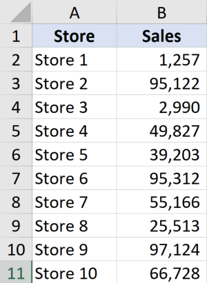
Suppose you have a data set as shown below, and you want to calculate the range for the data in column B.
Below is the formula to calculate the range for this data set:
=MAX(B2:B11)-MIN(B2:B11)
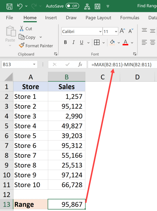
The above formula finds the maximum and the minimum value and gives us the difference.
Quite straightforward… isn’t it?
Calculate Conditional Range in Excel
In most practical cases, finding the range would not be as simple as just subtracting the minimum value from the maximum value
In real-life scenarios, you might also need to account for some conditions or outliers.
For example, you may have a data set where all the values are below 100, but there is one value that is above 500.
If you calculate arrange for this data set, it would lead to you making misleading interpretations of the data.
Thankfully, Excel has many conditional formulas that can help you sort out some of the anomalies.
Below I have a data set where I need to find the range for the sales values in column B.
If you look closely at this data, you would notice that there are two stores where the values are quite low (Store 1 and Store 3).
This could be because these are new stores or there were some external factors that impacted the sales for these specific stores.
While calculating the range for this data set, it might make sense to exclude these newer stores and only consider stores where there are substantial sales.
In this example, let’s say I want to ignore all those stores where the sales value is less than 20,000.
Below is the formula that would find the range with the condition:
=MAX(B2:B11)-MINIFS(B2:B11,B2:B11,">20000")
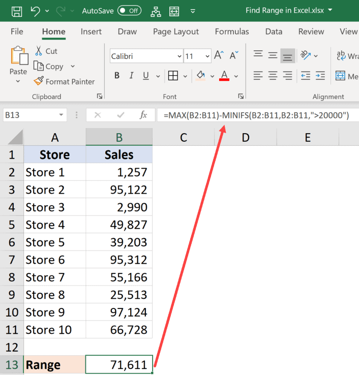
In the above formula, instead of using the MIN function, I have used the MINIFS function (it’s a new function in Excel 2019 and Microsoft 365).
This function finds the minimum value if the criteria mentioned in it are met. In the above formula, I specified the criteria to be any value that is more than 20,000.
So, the MINIFS function goes through the entire data set, but only considers those values that are more than 20,000 while calculating the minimum value.
This makes sure that values lower than 20,000 are ignored and the minimum value is always more than 20,000 (hence ignoring the outliers).
Note that the MINIFS is a new function in Excel is available only in Excel 2019 and Microsoft 365 subscription. If you’re using prior versions, you would not have this function (and can use the formula covered later in this tutorial)
If you don’t have the MINIF function in your Excel, use the below formula that uses a combination of IF function and MIN function to do the same:
=MAX(B2:B11)-MIN(IF(B2:B11>20000,B2:B11))
Just like I have used the conditional MINIFS function, you can also use the MAXIFS function if you want to avoid data points that are outliers in the other direction (i.e., a couple of large data points that can skew the data)
So, this is how you can quickly find the range in Excel using a couple of simple formulas.
I hope you found this tutorial useful.
Other Excel tutorials you may like:
- How to Calculate Standard Deviation in Excel
- How to Calculate Square Root in Excel
- How to Calculate and Format Percentages in Excel
Find Range in Excel (Table of Contents)
- Range in Excel
- How to Find Range in Excel?
Range in Excel
Whenever we talk about the range in excel, it can be one cell or can be a collection of cells. It can be the adjacent cells or non-adjacent cells in the dataset.
What is Range in Excel & its Formula?
A range is the collection of values spread between the Maximum value and the Minimum value. A range is a difference between the Largest (maximum) value and the Shortest (minimum) value in a given dataset in mathematical terms.
Range defines the spread of values in any dataset. It calculates by a simple formula like below:
Range = Maximum Value – Minimum Value
How to Find Range in Excel?
Finding a range is a very simple process, and it is calculated using the Excel in-built functions MAX and MIN. Let’s understand the working of finding a range in excel with some examples.
You can download this Find Range Excel Template here – Find Range Excel Template
Range in Excel – Example #1
We have given below a list of values:
23, 11, 45, 21, 2, 60, 10, 35
The largest number in the above-given range is 60, and the smallest number is 2.
Thus, the Range = 60-2 = 58
Explanation:
- In this above example, the Range is 58 in the given dataset, which defines the span of the dataset. It gave you a visual indication of the range as we are looking for the highest and smallest point.
- If the dataset is large, it gives you the widespread of the result.
- If the dataset is small, it gives you a closely centered result.
A process of defining the range in Excel
For defining the range, we need to find out the maximum and minimum values of the dataset. In this process, two function plays a very important role. They are:
- MAX
- MIN
Use of MAX function:
Let’s take an example to understand the usage of this function.
Range in Excel – Example #2
We have given some set of values:
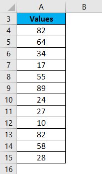
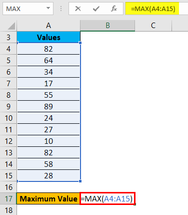
For finding the maximum value from the dataset, we will apply here the MAX function as below screenshot:
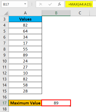
Hit enter, and it will give you the maximum value. The result is shown below:
Range in Excel – Example #3
Use of MIN function:
Let’s take the same above dataset to understand the usage of this function.
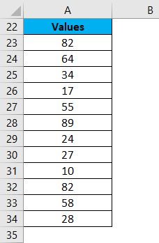
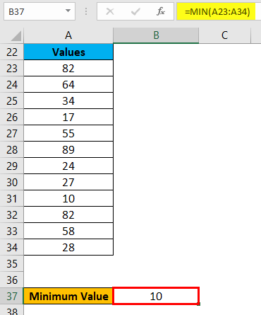
For calculating the minimum value from the given dataset, we will apply the MIN function here as per the below screenshot.
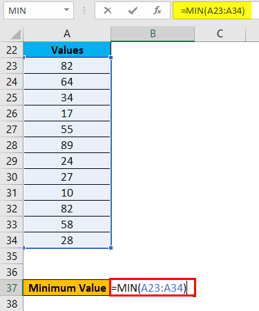
Press ENTER key, and it will give you the minimum value. The result is given below:
Now you can find out the range of the dataset after taking the difference between Maximum and Minimum value.
We can reduce the steps for calculating the range of a dataset by using the MAX and MIN functions together in one line.
For this, we again take an example to understand the process.
Range in Excel – Example #4
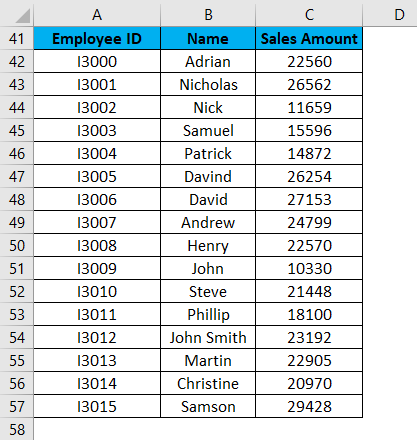
Let’s assume the below dataset of a company employee with their achieved sales target.
Now for identifying the span of sales amount in the above dataset, we will calculate the range. For this, we will follow the same procedure as we did in the above examples.
We will apply the MAX and MIN functions for calculating the Maximum and Minimum sales amount in the data.
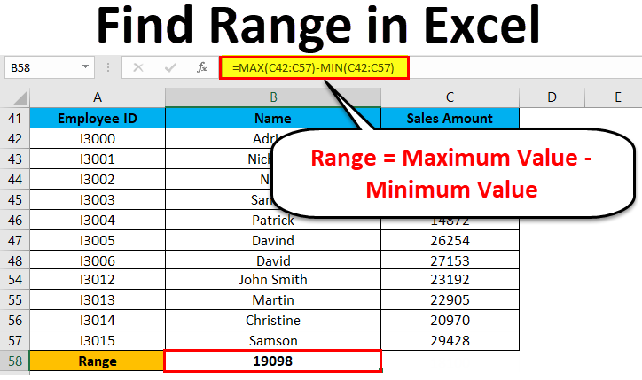
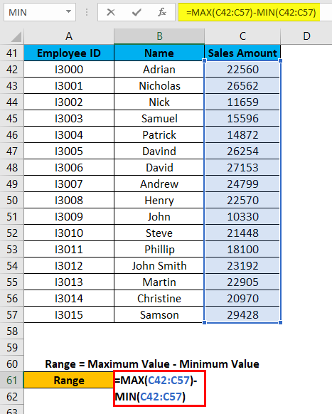
For finding the range of sales amount, we will apply the below formula:
Range = Maximum Value – Minimum Value
Refer to the below screenshot:
Press Enter key, and it will give you the range of the dataset. The result is shown below:
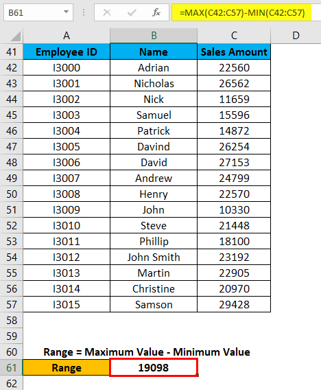
As we can see in the above screenshot, we applied the MAX and MIN formulas in one line, and by calculating their results difference, we found the range of the dataset.
Things to Remember
- If the values are available in the non-adjacent cells, you want to find out the range; you can pass the cell address individually, separated with a comma as an argument of the MAX and MIN functions.
- We can reduce the steps for calculating the range by applying MAX and MIN functions in one line. (Refer to Example 4 for your reference)
Recommended Articles
This has been a guide to Range in Excel. Here we discuss how to find Range in Excel along with excel examples and downloadable excel template. You may learn more about Excel from the following articles –
- Excel Function for Range
- Excel Named Range
- VBA Range
- VBA Selecting Range
We usually require certain metrics to understand the data that we are working with. There are a number of such representative metrics, like the average, the median, etc. Among these metrics, an often-used value is the ‘Range’.
In this tutorial, we will show you two easy ways in which you can find the range of a series of numbers in Excel:
- Using a formula with the MIN and MAX built-in functions
- Using a formula with the SMALL and LARGE built-in functions
What is Range and How is it Calculated?
The range is a measure of the spread of values in a series. In other words, it is the variation between the upper and lower limits of the series on a particular scale.
To find the range of a set of numbers, you need to find the difference between the largest and smallest numbers.
For example, if you have a series of numbers {4,2,6,5,3} then the range can be calculated as follows:
Range = largest value - smallest value
= 6 – 2
Calculation of the range is a very simple process, requiring three basic arithmetic operations:
- Finding the largest value
- Finding the smallest value
- Finding the difference between the two
Given below are two methods to quickly calculate the range of a set of numbers in Excel. To demonstrate both methods, we will use the following dataset:

Finding the Range in Excel with MIN and MAX Functions
The first way to find the range is to use a combination of the MIN and MAX functions.
The MIN Function
The Excel MIN function returns the smallest numeric value in a range of values. The syntax for the MIN function is as follows:
=MIN (number1, [number2], ...)
Here,
- number1 can be a numeric value, a reference to a numeric value, or a range of numeric values.
- number2,… is optional. It can be a numeric value, a reference to a numeric value, or a range of numeric values.
For example, to find the minimum value of numbers in the range B2:B7, you will write the MIN function as follows:
=MIN(B2:B7)
The MAX Function
The Excel MAX function returns the largest numeric value in a range of values. The syntax for the MAX function is as follows:
=MAX (number1, [number2], ...)
Here,
- number1 can be a numeric value, a reference to a numeric value, or a range of numeric values.
- number2, … is optional. It can be a numeric value, a reference to a numeric value, or a range of numeric values.
For example, to find the maximum value of numbers in the range B2:B7, you will write the MAX function as follows:
=MAX(B2:B7)
Note: Both MIN and MAX functions ignore empty cells, logical values like TRUE and FALSE, as well as text values.
Using the MIN and MAX functions to Find the Range of A Series
To find the range of values in the given dataset, we can use the MIN and MAX functions as follows:
- Select the cell where you want to display the range (B8 in our example).
- Type in the formula: =MAX(B2:B7)-MIN(B2:B7)
- Press the Return key.

Note: You can replace the reference B2:B7 with reference to the cells containing the values you want to calculate the range for.
Explanation of the Formula
The formula simply performed the basic steps required to calculate the range:
- Finding the largest value: =MAX(B2:B7)
- Finding the smallest value: =MIN(B2:B7)
- Finding the difference between the two: =MAX(B2:B7) – MIN(B2:B7)
Finding the Range in Excel with SMALL and LARGE Functions
The second way to find the range is to use a combination of the SMALL and LARGE function.
The SMALL Function
The Excel SMALL function returns the ‘n-th smallest value’ in a range of values. So you can use it to find the 1st smallest value, 2nd smallest value, 3rd smallest value, and so on.
The syntax for the SMALL function is as follows:
=SMALL (array, n)
Here,
- array is the range of cells that you want to find the n-th smallest value from.
- n is an integer that specifies the position from the smallest value, i.e. the nth position.
For example, to find the 3rd smallest value in the range B2:B7, you will write the SMALL function as follows:
=SMALL(B2:B7,3)
Similarly, to find the smallest value in the range B2:B7, you will write the function as follows:
=SMALL(B2:B7, 1)
Notice the above function gives a result equivalent to the function:
=MIN(A2:A7)
The LARGE Function
The Excel LARGE function returns the ‘n-th largest value’ in a range of values. So you can use it to find the 1st largest value, 2nd largest value, 3rd largest value and so on.
The syntax for the LARGE function is as follows:
= LARGE (array, n)
Here,
- array is the range of cells that you want to find the n-th largest value from.
- n is an integer that specifies the position from the largest value, i.e. the nth position.
For example, to find the 3rd largest value in the range B2:B7, you will write the LARGE function as follows:
= LARGE (B2:B7,3)
Similarly, to find the largest value in the range B2:B7, you will write the function as follows:
= LARGE (B2:B7, 1)
Notice the above function gives a result equivalent to the function:
=MAX(B2:B7)
Note: In cases where you’re working with large volumes of data, using the MIN and MAX functions are more efficient to use than the SMALL and LARGE. This is because the SMALL and LARGE functions require more computing and resources.
Using the SMALL and LARGE functions to Find the Range of A Series
To find the range of values in the given dataset, we can use the SMALL and LARGE functions as follows:
- Select the cell where you want to display the range (B8 in our example).
- Type in the formula: =LARGE(B2:B7,1) – SMALL(B2:B7,1)
- Press the Return key.

Note: You can replace the reference B2:B7 with reference to the cells containing the values you want to calculate the range for.
Explanation of the Formula
The formula simply performed the basic steps required to calculate the range:
- Finding the largest value: = LARGE(B2:B7,1)
- Finding the smallest value: = SMALL(B2:B7,1)
- Finding the difference between the two: =LARGE(B2:B7,1)-SMALL(B2:B7,1)
Applications and Limitations of the Range
The range provides a great way for us to get a basic understanding of how spread out the numbers in the dataset are.
So, a higher range value means the data is quite spread out, while a smaller range value means the data is less spread out, or more concentrated.
It must be noted, though, that the range is a very crude measurement since it is quite sensitive to outliers.
A single value that is too high or too low can completely alter the range, giving an erroneous representation of the data. As such, it doesn’t always provide a true indication of the spread in the dataset.
Having said that, the range is easy to calculate. It only requires basic operations. So, it is a good way to help you get a very basic understanding of the nature of your data.
Other Excel tutorials you may also like:
- How to Calculate Standard Error In Excel
- How to Square a Number in Excel
- How to Use Pi (π) in Excel
- How to Calculate Antilog in Excel
- How to Use e in Excel | Euler’s Number in Excel
- How to Find Outliers in Excel
- How to Find Slope in Excel (Easy Formula)
- How to Find Percentile in Excel (PERCENTILE Function)
When an excel user talks about the range in excel, it is obvious that he/she must be referenced to the individual cell or to the collection of the cell within the excel worksheet.
People might get confused with the term ‘Range’ as it is used in mathematics also. (In mathematics- Range is the value that lies between the given data’s minimum and maximum value).
In the blog, we will help you to understand how to find range in excel, range in excel formula, and what the difference is between excel table vs range. But before proceeding to more details about range in excel, let us know what the range is.
What is the Range?
As we have already mentioned that when a user talks about the range in excel, then there is a possibility that he/she talks about the single cell or the group of cells.
Moreover, the range can be non-adjacent or adjacent cells within the dataset.
Now, the question is, what is the range? Well, a range is the combination of various value spreads that lies between the minimum and maximum value. Or we can say that range is used to define the spread of values within the datasets.
The basic formula of the range is as:
Range = Maximum Value – Minimum Value
For example, suppose you select 10 different numbers randomly within the list of excel. Now, to find out the range of the numbers, you require to find out the maximum or upper and minimum or lower value using MAX & MIN functions.
When you get the minimum and maximum value of the number, then subtract the MIN value from the MAX value. The result is known as the range.
What are the two types of ranges used in Excel?
| Symmetrical Range | Irregular Range |
| It is the range of the cells that are located at the adjacent position to one another. This kind of range usually looks like a rectangle or square within the spreadsheet whenever they are highlighted. The below image shows the range as (A1:C4). | A range consists of cells that are not contiguous or might have irregular geometrical shapes whenever they are highlighted. In the below image, the highlighted cells are: (A1:C4, E1, E4, B6). |
To know the exact procedure of the range in excel, let’s take an example. Suppose you have a list of different values as:
19, 12, 48, 20, 5, 60, 15, 39
Now, you can see that the largest number in the given dataset is 60, whereas the smallest number of the dataset is 5.
Therefore, the range will be 60 – 5 = 55.
This is how you calculate the range of the dataset in mathematics with a simple formula. The same procedure you need to follow in excel. The only difference is that you can check the range using the MIN and MAX function in the excel worksheet.
How to use range in excel formula?
Several businesses do not have enough time to waste sorting the data through columns and rows. The rows and columns have the lowest and highest values of sales, revenues, or other useful information.
The lowest and highest figures within the data group are useful for accurate decision-making, forecasting, and budgeting.
It is known to all that excel provides various ways for writing the range formulas that can work as per the user needs and required times. So, let’s check the range in excel formula or how to find range in excel.
MIN and MAX Formula
Suppose a manager keeps the product sale data that include model, unit price, state, number of units, and the total revenue of every product/state.
The product sale data of the previous sale will be as follows:
Now, you can find which product has the greatest and smallest demand. Using the below formula mentioned, you can easily check the MAX() and MIN() values.
- In cell B16, type “=MAX(C2:C13)”.
- In cell B15, type “=MIN(C2:C13)”.
Now, you will notice that the smallest number of units sold in the respective state is 102 tablets in Iowa, whereas the largest sold is 450 laptops in Illinois.
Bottom k and Top k formula
Suppose you have multiple data that has details as three different lowest-selling items. You can use the SMALL () functions, but before that, you require two factors:
- A similar list or range of the values that you will use for MIN().
- The specific value of k, which is the required position from the bottom. [If you want to check the smallest value, then the value of k will be k = 1. For the second smallest value, k = 2, and so on.]
NOTES:
- The LARGE() with k = 1 provides a similar result as that of MAX().
- Whereas the SMALL() with k = 1 will give the same output as MIN().
3. Conditional Maximum and Minimum Formula
Sometimes, you need to check the minimum value, which can easily meet the particular criteria.
Let’s take an example; suppose you require to check the lowest units sold in the spring quarter.
Here, you can use COUNTIF(), SUMIF(), and other conditional formulas. [But there is no MAXIF() & MINIF(); therefore, you need to create a different array to find Max and Mini statement functions]. This array formula will help the user evaluate the specific cells’ range rather than the individual cell.
Usually, the IF() formula is used to test the real value of the individual cell. But users can use it to evaluate every cell within the range.
When you use the array formula and press enter, it will show #VALUE!. Therefore, always keep in mind that you have to select CTRL+SHIFT+ENTER once you finish the array formula.
In this example, you can find the minimum value of the desktops. For this, write the match value in the cell to compare it with the functions.
Type “desktop” in B18. Now, the formula compares the testing cell reference. Now, type IF() statement as: “=MIN(IF(B2:B13=B18,C2:C13))” and select the <CTRL>+<SHIFT>+<ENTER>.
The calculated value of the three formulas will display in rows 18, 19, and 20. This shows that the minimum sell number is of laptops, desktops, and tablets.
Moreover, users can use the identical formula with MAX() to get the largest product sold.
This is how to find range in excel !!!
A Comparison Table: Excel Table vs Range
We know that the range of cells is used to check the list’s minimum and maximum values. And the list is created in the form of a table.
But there is a major difference between the table and the range.
Moreover, there is a necessity that users must know the difference between a table and the range.
Do not worry; we have provided a comparison table of excel table vs range that helps you to know the difference.
| Table | Range |
| The format of the table can be changed easily by the user. | The format of the range can change manually by the user. |
| The table feature has the slicer command. | The slicer command is not available in the range. |
| The header of the table has the filter button. | If a user wants to filter a range, then he/she can do it using the Filter command available in the Data Ribbon. |
| When a user scrolls the table down, the header easily replaces the common column headings. | In the case of range, the headers can not be replaced by the column headings whenever the user scrolls down. |
| Users can expand the table very easily. | Users can not expand the range of the data. |
| Structured References easily supported by the table. | Structured References are not supported by the range. |
| The tables in excel are treated as the Object. | In excel, the range does not treat as an Object. |
| If a user wants to use a formula in a column, then the formula can be copied to other cells as well within the same cell. | Suppose a user wants to use a formula in a column. He/she needs to double click on the AutoFill Handle tool, then copy the same formula to each column. You have to keep in mind that the formula does not get copied by itself. |
Conclusion
Basically, the range is the difference between the minimum limit and the maximum limit of the available numbers in excel. We have provided the details about how to find range in excel using three different methods.
Users can use it to check the maximum and minimum values from the list. Moreover, users might be confused with the excel table and range, so we have provided a comparison table of excel table vs range. Check the table to know the difference.
If you still have any issue or query regarding how to find range in excel, comment in the below section. We will help you to get the details about the range of cells in excel.
We always help our readers with their queries in the best possible way. So, do not waste your time here and there; use the above-mentioned excel formulas to enhance your skills!!!
if you have a question about who can do my excel assignment, then contact our excel assignments experts.
![]()
Download Article
![]()
Download Article
Microsoft Excel makes it possible to get all kinds of useful information out of a set of data. With a few quick clicks, you can calculate your range.
Steps
-

1
Find the maximum value of the data.
- To do this, pick a cell where you want the maximum to display (for example, maybe two cells above where you’ll put the range).
- Type {{{1}}} and specify the cells you’re trying to find the range for. For example, you might write {{{1}}} or {{{1}}}.
- Press ↵ Enter
-
2
Find the minimum value of the data.
- To do this, pick a cell where you want the minimum to display (for example, maybe one cell above where you’ll put the range, below the maximum).
- Type Min and specify the cells again. For example, you might write MIN(J7:T1) or MIN(A1:A500).
- Press ↵ Enter
Advertisement
-
3
Find the Range.
- Type = in the call for the range (possibly below the other two).
- Type in the cell number that you used for typing the maximum number first — for example, B1.
- Then type a -.
- Type in the minimum cell number. For example, B2. Your formula should read something like: =B1-B2
- Press ↵ Enter


Advertisement
Ask a Question
200 characters left
Include your email address to get a message when this question is answered.
Submit
Advertisement
-
Every command must start with an equal sign ( = ).
-
Commands must be in upper case.
-
Command suggestions will come up when you click on the Fx in front of the command bar.
Thanks for submitting a tip for review!
Advertisement
About This Article
Thanks to all authors for creating a page that has been read 45,096 times.
Is this article up to date?
Содержание
- How to Find Range in Excel (Easy Formulas)
- What is a Range?
- How to Calculate Range in Excel?
- Calculate Conditional Range in Excel
- Метод Range.Find (Excel)
- Синтаксис
- Параметры
- Возвращаемое значение
- Примечания
- Примеры
- Поддержка и обратная связь
- Range in Excel
- Range in Excel
- How to Find Range in Excel?
- Range in Excel – Example #1
- Range in Excel – Example #2
- Range in Excel – Example #3
- Range in Excel – Example #4
- Things to Remember
- Recommended Articles
How to Find Range in Excel (Easy Formulas)
Normally, when I use the word range in my tutorials about Excel, it’s a reference to a cell or a collection of cells in the worksheet.
But this tutorial is not about that range.
A ‘Range’ is also a mathematical term that refers to the range in a data set (i.e., the range between the minimum and the maximum value in a given dataset)
In this tutorial, I will show you really simple ways to calculate the range in Excel.
What is a Range?
In a given data set, the range of that data set would be the spread of values in that data set.
To give you a simple example, if you have a data set of student scores where the minimum score is 15 and the maximum score is 98, then the spread of this data set (also called the range of this data set) would be 73
‘Range’ is nothing but the difference between the maximum and the minimum value of that data set.
How to Calculate Range in Excel?
If you have a list of sorted values, you just have to subtract the first value from the last value (assuming that the sorting is in the ascending order).
But in most cases, you would have a random data set where it’s not already sorted.
Finding the range in such a data set is quite straightforward as well.
Excel has the functions to find out the maximum and the minimum value from a range (the MAX and the MIN function).
Suppose you have a data set as shown below, and you want to calculate the range for the data in column B.
Below is the formula to calculate the range for this data set:
The above formula finds the maximum and the minimum value and gives us the difference.
Quite straightforward… isn’t it?
Calculate Conditional Range in Excel
In most practical cases, finding the range would not be as simple as just subtracting the minimum value from the maximum value
In real-life scenarios, you might also need to account for some conditions or outliers.
For example, you may have a data set where all the values are below 100, but there is one value that is above 500.
If you calculate arrange for this data set, it would lead to you making misleading interpretations of the data.
Thankfully, Excel has many conditional formulas that can help you sort out some of the anomalies.
Below I have a data set where I need to find the range for the sales values in column B.
If you look closely at this data, you would notice that there are two stores where the values are quite low (Store 1 and Store 3).
This could be because these are new stores or there were some external factors that impacted the sales for these specific stores.
While calculating the range for this data set, it might make sense to exclude these newer stores and only consider stores where there are substantial sales.
In this example, let’s say I want to ignore all those stores where the sales value is less than 20,000.
Below is the formula that would find the range with the condition:
In the above formula, instead of using the MIN function, I have used the MINIFS function (it’s a new function in Excel 2019 and Microsoft 365).
This function finds the minimum value if the criteria mentioned in it are met. In the above formula, I specified the criteria to be any value that is more than 20,000.
So, the MINIFS function goes through the entire data set, but only considers those values that are more than 20,000 while calculating the minimum value.
This makes sure that values lower than 20,000 are ignored and the minimum value is always more than 20,000 (hence ignoring the outliers).
Note that the MINIFS is a new function in Excel is available only in Excel 2019 and Microsoft 365 subscription. If you’re using prior versions, you would not have this function (and can use the formula covered later in this tutorial)
If you don’t have the MINIF function in your Excel, use the below formula that uses a combination of IF function and MIN function to do the same:
Just like I have used the conditional MINIFS function, you can also use the MAXIFS function if you want to avoid data points that are outliers in the other direction (i.e., a couple of large data points that can skew the data)
So, this is how you can quickly find the range in Excel using a couple of simple formulas.
I hope you found this tutorial useful.
Other Excel tutorials you may like:
Источник
Метод Range.Find (Excel)
Находит определенные сведения в диапазоне.
Хотите создавать решения, которые расширяют возможности Office на разнообразных платформах? Ознакомьтесь с новой моделью надстроек Office. Надстройки Office занимают меньше места по сравнению с надстройками и решениями VSTO, и вы можете создавать их, используя практически любую технологию веб-программирования, например HTML5, JavaScript, CSS3 и XML.
Синтаксис
выражение.Find (What, After, LookIn, LookAt, SearchOrder, SearchDirection, MatchCase, MatchByte, SearchFormat)
выражение: переменная, представляющая объект Range.
Параметры
| Имя | Обязательный или необязательный | Тип данных | Описание |
|---|---|---|---|
| What | Обязательный | Variant | Искомые данные. Может быть строкой или любым типом данных Microsoft Excel. |
| After | Необязательный | Variant | Ячейка, после которой нужно начать поиск. Соответствует положению активной ячейки, когда поиск выполняется из пользовательского интерфейса. |
Обратите внимание, что параметр After должен быть одной ячейкой в диапазоне. Помните, что поиск начинается после этой ячейки; указанная ячейка не входит в область поиска, пока метод не возвращается обратно в эту ячейку.
Если не указать этот аргумент, поиск начинается после ячейки в левом верхнем углу диапазона. LookIn Необязательный Variant Может быть одной из следующих констант XlFindLookIn: xlFormulas, xlValues, xlComments или xlCommentsThreaded. LookAt Необязательный Variant Может быть одной из следующих констант XlLookAt: xlWhole или xlPart. SearchOrder Необязательный Variant Может быть одной из следующих констант XlSearchOrder: xlByRows или xlByColumns. SearchDirection Необязательный Variant Может быть одной из следующих констант XlSearchDirection: xlNext или xlPrevious. MatchCase Необязательный Variant Значение True, чтобы выполнять поиск с учетом регистра. Значение по умолчанию — False. MatchByte Необязательный Variant Используется только в том случае, если выбрана или установлена поддержка двухбайтовых языков. Значение True, чтобы двухбайтовые символы сопоставлялись только с двухбайтовым символами. Значение False, чтобы двухбайтовые символы сопоставлялись с однобайтовыми эквивалентами. SearchFormat Необязательный Variant Формат поиска.
Возвращаемое значение
Объект Range, представляющий первую ячейку, в которой обнаружены требуемые сведения.
Примечания
Этот метод возвращает значение Nothing, если совпадения не найдены. Метод Find не влияет на выделенный фрагмент или активную ячейку.
Параметры для аргументов LookIn, LookAt, SearchOrder и MatchByte сохраняются при каждом использовании этого метода. Если не указать значения этих аргументов при следующем вызове метода, будут использоваться сохраненные значения. Установка этих аргументов изменяет параметры в диалоговом окне Найти, а изменение параметров в диалоговом окне Найти приводит к изменению сохраненных значений, которые используются, если опустить аргументы. Чтобы избежать проблем, устанавливайте эти аргументы явным образом при каждом использовании этого метода.
Для повторения поиска используйте методы FindNext и FindPrevious.
Когда поиск достигает конца указанного диапазона поиска, он возвращается в начало диапазона. Чтобы остановить поиск при этом возврате, сохраните адрес первой найденной ячейки, а затем проверьте адрес каждой последующей найденной ячейки, сравнив его с этим сохраненным адресом.
Чтобы найти ячейки, отвечающие более сложным шаблонам, используйте инструкцию For Each. Next с оператором Like. Например, следующий код выполняет поиск всех ячеек в диапазоне A1:C5, где используется шрифт, имя которого начинается с букв Cour. Когда Microsoft Excel находит соответствующее значение, шрифт изменяется на Times New Roman.
Примеры
В этом примере показано, как найти все ячейки в диапазоне A1:A500 на листе 1, содержащие значение 2, и изменить значение ячейки на 5. Таким образом, значения 1234 и 99299 содержали 2 и оба значения ячеек станут 5.
В этом примере показано, как найти все ячейки в диапазоне A1:A500 на листе 1, содержащие подстроку «abc», и изменить ее на «xyz».
Поддержка и обратная связь
Есть вопросы или отзывы, касающиеся Office VBA или этой статьи? Руководство по другим способам получения поддержки и отправки отзывов см. в статье Поддержка Office VBA и обратная связь.
Источник
Range in Excel
Find Range in Excel (Table of Contents)
Range in Excel
Whenever we talk about the range in excel, it can be one cell or can be a collection of cells. It can be the adjacent cells or non-adjacent cells in the dataset.
Excel functions, formula, charts, formatting creating excel dashboard & others
What is Range in Excel & its Formula?
A range is the collection of values spread between the Maximum value and the Minimum value. A range is a difference between the Largest (maximum) value and the Shortest (minimum) value in a given dataset in mathematical terms.
Range defines the spread of values in any dataset. It calculates by a simple formula like below:
How to Find Range in Excel?
Finding a range is a very simple process, and it is calculated using the Excel in-built functions MAX and MIN. Let’s understand the working of finding a range in excel with some examples.
Range in Excel – Example #1
We have given below a list of values:
23, 11, 45, 21, 2, 60, 10, 35
The largest number in the above-given range is 60, and the smallest number is 2.
Thus, the Range = 60-2 = 58
Explanation:
- In this above example, the Range is 58 in the given dataset, which defines the span of the dataset. It gave you a visual indication of the range as we are looking for the highest and smallest point.
- If the dataset is large, it gives you the widespread of the result.
- If the dataset is small, it gives you a closely centered result.
A process of defining the range in Excel
For defining the range, we need to find out the maximum and minimum values of the dataset. In this process, two function plays a very important role. They are:
Use of MAX function:
Let’s take an example to understand the usage of this function.
Range in Excel – Example #2
We have given some set of values:
For finding the maximum value from the dataset, we will apply here the MAX function as below screenshot:
Hit enter, and it will give you the maximum value. The result is shown below:
Range in Excel – Example #3
Use of MIN function:
Let’s take the same above dataset to understand the usage of this function.
For calculating the minimum value from the given dataset, we will apply the MIN function here as per the below screenshot.
Press ENTER key, and it will give you the minimum value. The result is given below:
Now you can find out the range of the dataset after taking the difference between Maximum and Minimum value.
We can reduce the steps for calculating the range of a dataset by using the MAX and MIN functions together in one line.
For this, we again take an example to understand the process.
Range in Excel – Example #4
Let’s assume the below dataset of a company employee with their achieved sales target.
Now for identifying the span of sales amount in the above dataset, we will calculate the range. For this, we will follow the same procedure as we did in the above examples.
We will apply the MAX and MIN functions for calculating the Maximum and Minimum sales amount in the data.
For finding the range of sales amount, we will apply the below formula:
Range = Maximum Value – Minimum Value
Refer to the below screenshot:
Press Enter key, and it will give you the range of the dataset. The result is shown below:
As we can see in the above screenshot, we applied the MAX and MIN formulas in one line, and by calculating their results difference, we found the range of the dataset.
Things to Remember
- If the values are available in the non-adjacent cells, you want to find out the range; you can pass the cell address individually, separated with a comma as an argument of the MAX and MIN functions.
- We can reduce the steps for calculating the range by applying MAX and MIN functions in one line. (Refer to Example 4 for your reference)
Recommended Articles
This has been a guide to Range in Excel. Here we discuss how to find Range in Excel along with excel examples and downloadable excel template. You may learn more about Excel from the following articles –
Источник
So, you’ve named a range of cells, and … perhaps you forgot the location. You can find a named range by using the Go To feature—which navigates to any named range throughout the entire workbook.
-
You can find a named range by going to the Home tab, clicking Find & Select, and then Go To.
Or, press Ctrl+G on your keyboard.
-
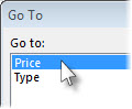
In the Go to box, double-click the named range you want to find.
Notes:
-
The Go to popup window shows named ranges on every worksheet in your workbook.
-
To go to a range of unnamed cells, press Ctrl+G, enter the range in the Reference box, and then press Enter (or click OK). The Go to box keeps track of ranges as you enter them, and you can return to any of them by double-clicking.
-
To go to a cell or range on another sheet, enter the following in the Reference box: the sheet name together with an exclamation point and absolute cell references. For example: sheet2!$D$12 to go to a cell, and sheet3!$C$12:$F$21 to go to range.
-
You can enter multiple named ranges or cell references in the Reference box. Separating each with a comma, like this: Price, Type, or B14:C22,F19:G30,H21:H29. When you press Enter or click OK, Excel will highlight all the ranges.
More about finding data in Excel
-
Find or replace text and numbers on a worksheet
-
Find merged cells
-
Remove or allow a circular reference
-
Find cells that contain formulas
-
Find cells that have conditional formats
-
Locate hidden cells on a worksheet
Need more help?
A data range in Excel is simply a collection of two or more cells; the cells are not required to be next to each other.
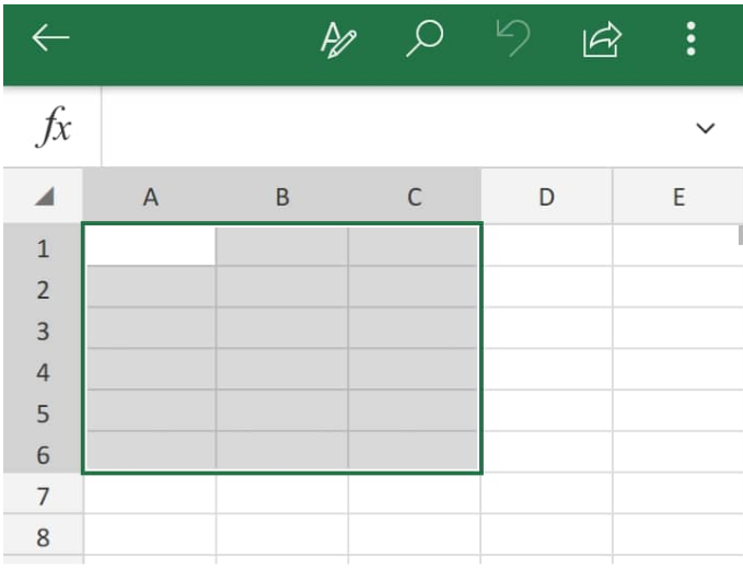 Figure 1. Cell Range in Excel
Generic Formula
=RANGE(max value-min value)
- Max value = Largest number value in the selected range
- Min value = Smallest number value in the selected range
We can select a cell range in Excel by holding down the CTRL keyboard key and then clicking on each individual cell that we want to be included in the range. The data range in Excel of a particular set of data gives us a simple idea of the distribution of values that it contains.
How to Calculate Range in Excel
Finding Range in Excel is a simple task which requires us to subtract the Minimum value of numbers contained in the selected cells from the Maximum value.
Here’s how to calculate range in Excel;
- We begin by finding the MAX value of a set of data in our worksheet;
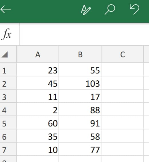 Figure 2. Data Values in Excel
To determine the MAX value for the data set above we will use the MAX Function in Excel.
- The MAX formula we will enter into cell B9 of our worksheet example is as follows;
=MAX(A1:B7)
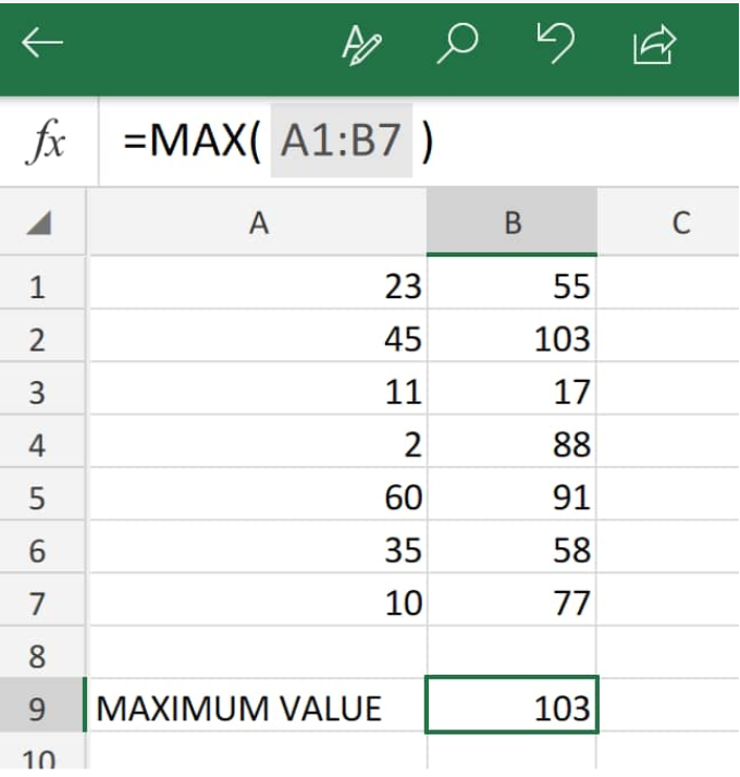 Figure 3. MAX Value in Excel
The range function in Excel returned the MAX value in the selected range of data above (A1:B7), as103.
- Next, we have to determine the MIN value in our data set.
The MIN formula we will enter into cell B9 of our worksheet example is as follows;
=MIN(A1:B7)
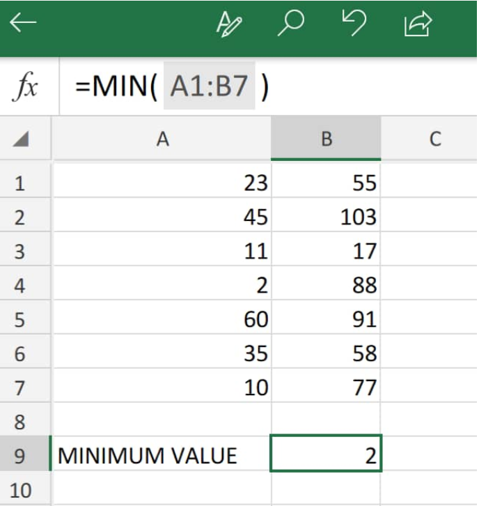 Figure 4. MIN Value in Excel
The range function in Excel returned the MIN value in the selected range of data above (A1:B7), as 2.
Since we now know how to use the range function in Excel to calculate MAX and MIN values, let us now demonstrate how to find the range in Excel by subtracting the MIN value from the MAX value in the following data set;
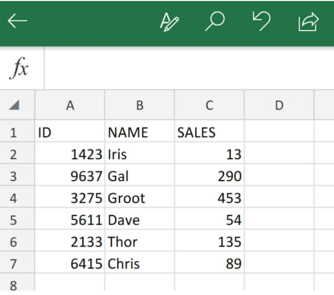 Figure 5. Data Set in Excel
- The Excel range formula we will enter into cell B9 of our worksheet example is as follows;
=MAX(C2:C7)-MIN(C2-C7)
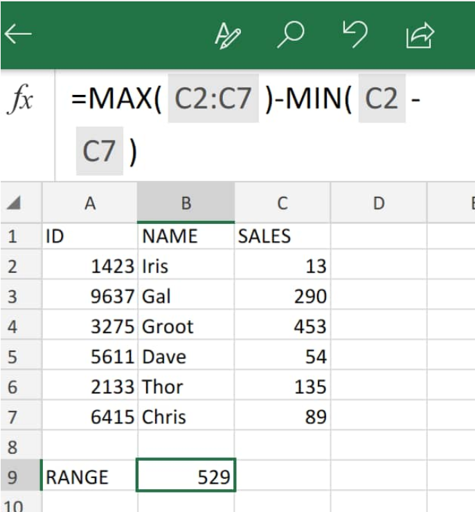 Figure 6. Finding Range in Excel
The Excel range function returned 529 as the total range value after subtracting the MIN value from the MAX value in the data set above.
Instant Connection to an Excel Expert
Most of the time, the problem you will need to solve will be more complex than a simple application of a formula or function. If you want to save hours of research and frustration, try our live Excelchat service! Our Excel Experts are available 24/7 to answer any Excel question you may have. We guarantee a connection within 30 seconds and a customized solution within 20 minutes.
VBA Excel. Метод Find объекта Range
Метод Find объекта Range для поиска ячейки по ее данным в VBA Excel. Синтаксис и компоненты. Знаки подстановки для поисковой фразы. Простые примеры.
Предназначение и синтаксис метода Range.Find
Метод Find объекта Range предназначен для поиска ячейки и сведений о ней в заданном диапазоне по ее значению, формуле и примечанию. Чаще всего этот метод используется для поиска в таблице ячейки по слову, части слова или фразе, входящей в ее значение.
Синтаксис метода Range.Find
Expression – это переменная или выражение, возвращающее объект Range, в котором будет осуществляться поиск.
В скобках перечислены параметры метода, среди них только What является обязательным.
Метод Range.Find возвращает объект Range, представляющий из себя первую ячейку, в которой найдена поисковая фраза (параметр What). Если совпадение не найдено, возвращается значение Nothing.
Параметры метода Range.Find
| Наименование | Описание |
| Обязательный параметр | |
| What | Данные для поиска, которые могут быть представлены строкой или другим типом данных Excel. Тип данных параметра – Variant. |
| Необязательные параметры | |
| After | Ячейка, после которой следует начать поиск. |
| LookIn | Уточняет область поиска. Список констант xlFindLookIn:
|
| LookAt | Поиск частичного или полного совпадения. Список констант xlLookAt:
|
| SearchOrder | Определяет способ поиска. Список констант xlSearchOrder:
|
| SearchDirection | Определяет направление поиска. Список констант xlSearchDirection:
|
| MatchCase | Определяет учет регистра:
|
| MatchByte | Условия поиска при использовании двухбайтовых кодировок:
|
| SearchFormat | Формат поиска – используется вместе со свойством Application.FindFormat. |
* Примечания имеют две константы с одним значением. Проверяется очень просто: MsgBox xlComments и MsgBox xlNotes .
** Тесты показали неработоспособность метода Range.Find с константой xlFormulas в моей версии VBA Excel.
В справке Microsoft тип данных всех параметров, кроме SearchDirection, указан как Variant.
Знаки подстановки для поисковой фразы
Условные знаки в шаблоне поисковой фразы:
- ? – знак вопроса обозначает любой отдельный символ;
- * – звездочка обозначает любое количество любых символов, в том числе ноль символов;
Простые примеры
При использовании метода Range.Find в VBA Excel необходимо учитывать следующие нюансы:
- Так как этот метод возвращает объект Range (в виде одной ячейки), присвоить его можно только объектной переменной, объявленной как Variant, Object или Range, при помощи оператора Set.
- Если поисковая фраза в заданном диапазоне найдена не будет, метод Range.Find возвратит значение Nothing. Обращение к свойствам несуществующей ячейки будет генерировать ошибки. Поэтому, перед использованием результатов поиска, необходимо проверить объектную переменную на содержание в ней значения Nothing.
В примерах используются переменные:
- myPhrase – переменная для записи поисковой фразы;
- myCell – переменная, которой присваивается первая найденная ячейка, содержащая поисковую фразу, или значение Nothing, если поисковая фраза не найдена.
VBA Find
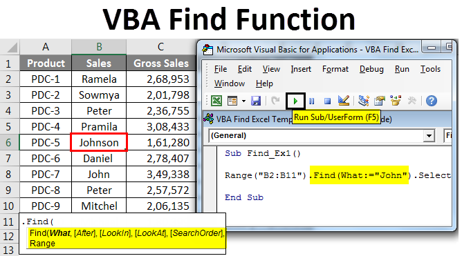
Excel VBA Find Function
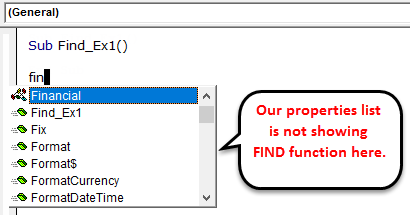
Who doesn’t know FIND method in excel? I am sure everybody knows who are dealing with excel worksheets. FIND or popular shortcut key Ctrl + F will find the word or content you are searching for in the entire worksheet as well as in the entire workbook. When you say find means you are finding in cells or ranges isn’t it? Yes, the correct find method is part of the cells or ranges in excel as well as in VBA.
Similarly, in VBA Find, we have an option called FIND function which can help us find the value we are searching for. In this article, I will take you through the methodology of FIND in VBA.
Valuation, Hadoop, Excel, Mobile Apps, Web Development & many more
Formula to Find Function in Excel VBA
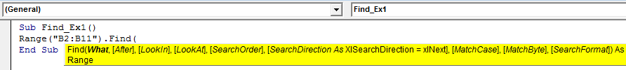
In regular excel worksheet, we simply type shortcut key Ctrl + F to find the contents. But in VBA we need to write a function to find the content we are looking for. Ok, let’s look at the FIND syntax then.

I know what is going on in your mind, you are lost by looking at this syntax and you are understanding nothing. But nothing to worry before I explain you the syntax let me introduce you to the regular search box.
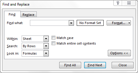
If you observe what is there in regular Ctrl + F, everything is there in VBA Find syntax as well. Now take a look at what each word in syntax says about.
What: Simply what you are searching for. Here we need to mention the content we are searching for.
After: After which cell you want to search for.
LookIn: Where to look for the thing you are searching For example Formulas, Values, or Comments. Parameters are xlFormulas, xlValues, xlComments.
LookAt: Whether you are searching for the whole content or only the part of the content. Parameters are xlWhole, xlPart.
SearchOrder: Are you looking in rows or Columns. xlByRows or xlByColumns.
SearchDirection: Are you looking at the next cell or previous cell. xlNext, xlPrevious.
MatchCase: The content you are searching for is case sensitive or not. True or False.
MatchByte: This is only for double-byte languages. True or False.
SearchFormat: Are you searching by formatting. If you are searching for format then you need to use Application.FindFormat method.
This is the explanation of the syntax of the VBA FIND method. Apart from the first parameter, everything is optional. In the examples section, we will see how to use this FIND method in VBA coding.
How to Use Excel VBA Find Function?
We will learn how to use a VBA Find Excel function with few examples.
VBA Find Function – Example #1
First up let me explain you a simple example of using FIND property and find the content we are looking for. Assume below is the data you have in your excel sheet.
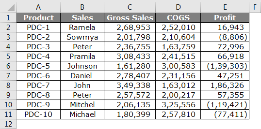
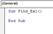
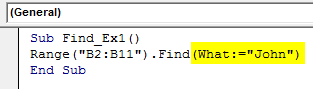
Step 1: From this, I want to find the name John, let’s open a Visual basic and start the coding.
Code:
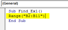
Step 2: Here you cannot start the word FIND, because FIND is part of RANGE property. So, firstly we need to mention where we are looking i.e. Range.
Step 3: So first mention the range where we are looking for. In our example, our range is from B2 to B11.
Code:
Step 4: After mentioning the range put a dot (.) and type FIND. You must see FIND property.
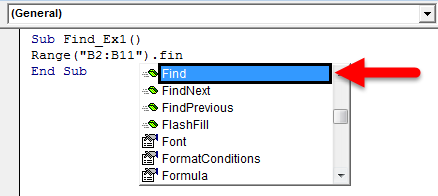
Step 5: Select the FIND property and open the bracket.
Step 6: Our first argument is what we are searching for. In order to highlight the argument we can pass the argument like this What:=, this would be helpful to identify which parameter we are referring to.
Code:
Step 7: The final part is after finding the word what we want to do. We need to select the word, so pass the argument as .Select.
Code:
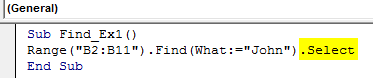
Step 8: Then run this code using F5 key or manually as shown in the figure, so it would select the first found word Johnson which contains a word, John.
VBA Find Function – Example #2
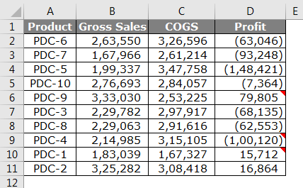
Now I will show you how to find the comment word using the find method. I have data and in three cells I have a comment.
Those cells having red flag has comments in it. From this comment, I want to search the word “No Commission”.
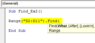
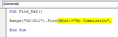
Step 1: Start code with mentioning the Range (“D2:D11”) and put a dot (.) and type Find
Code:
Step 2: In the WHAT argument type the word “No Commission”.
Code:
Step 3: Ignore the After part and select the LookIn part. In LookIn part we are searching this word in comments so select xlComments and then pass the argument as .Select
Code:
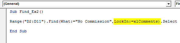
Step 4: Now run this code using F5 key or manually as shown in the figure so it will select the cell which has the comment “No Commission”. In D9 cell we have a mentioned comment.
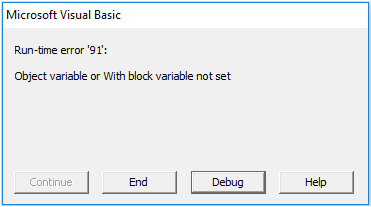
Deal with Error Values in Excel VBA Find
If the word we are searching for does not find in the range we have supplied VBA code which will return an error like this.
In order to show the user that the value you are searching for is not available, we need the below code.
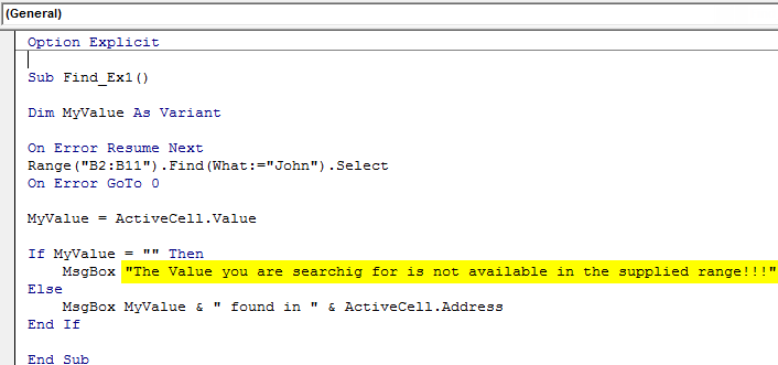
If the above code found value then it shows the value & cell address or else it will show the message as “The Value you are searching for is not available in the supplied range. ”.
Things to Remember
- VBA FIND is part of the RANGE property & you need to use the FIND after selecting the range only.
- In FIND first parameter is mandatory (What) apart from this everything else is optional.
- If you to find the value after specific cell then you can mention the cell in the After parameter of the Find syntax.
Recommended Articles
This has been a guide to VBA Find Function. Here we discussed VBA Find and how to use Excel VBA Find Function along with some practical examples and downloadable excel template. You can also go through our other suggested articles –
All in One Software Development Bundle (600+ Courses, 50+ projects)
Ron de Bruin
Excel Automation
Find value in Range, Sheet or Sheets with VBA
Copy the code in a Standard module of your workbook, if you just started with VBA see this page.
Where do I paste the code that I find on the internet
Find is a very powerful option in Excel and is very useful. Together with the Offset function you can also change cells around the found cell. Below are a few basic examples that you can use to in your own code.
Use Find to select a cell
The examples below will search in column A of a sheet named «Sheet1» for the inputbox value. Change the sheet name or range in the code to your sheet/range.
Tip: You can replace the inputbox with a string or a reference to a cell like this
FindString = «SearchWord»
Or
FindString = Sheets(«Sheet1»).Range(«D1»).Value
This example will select the first cell in the range with the InputBox value.
If you have more then one occurrence of the value this will select the last occurrence.
If you have date’s in column A then this example will select the cell with today’s date. Note : If your dates are formulas it is possible that you must change xlFormulas to xlValues in the example below. If your dates are values xlValues is not always working with some date formats.
Mark cells with the same value in column A in the B column
This example search in Sheets(«Sheet1») in column A for every cell with «ron» and use Offset to mark the cell in the column to the right. Note: you can add more values to the array MyArr.
Color cells with the same value in a Range, worksheet or all worksheets
This example color all cells in the range Sheets(«Sheet1»).Range(«B1:D100») with «ron». See the comments in the code if you want to use all cells on the worksheet. I use the color index in this example to give all cells with «ron» the color 3 (normal this is red)
Tip: For changing the Font color see the example lines below the macros.
Example for all worksheets in the workbook
Change the Font color instead of the Interior color
‘Change the fill color to «no fill» in all cells
.Interior.ColorIndex = xlColorIndexNone
‘Change the font in the column to Automatic
.Font.ColorIndex = 0
Rng.Interior.ColorIndex = myColor(I)
With
Rng.Font.ColorIndex = myColor(I)
Copy cells to another sheet with Find
The example below will copy all cells with a E-Mail Address in the range Sheets(«Sheet1»).Range(«A1:E100») to a new worksheet in your workbook. Note: I use xlPart in the code instead of xlWhole to find each cell with a @ character.
If you only want to replace values in your worksheet then you can use Replace manual (Ctrl+h) or use Replace in VBA. The code below replace ron for dave in the whole worksheet. Change xlPart to xlWhole if you only want to replace cells with only ron.
Excel VBA FIND Function (& how to handle if value NOT found)
Doing a CTRL + F on Excel to find a partial or exact match in the cell values, formulas or comments gives you a result almost instantly. In fact, it might even be faster to use this instead looping through multiple cells or rows in VBA. MS Excel’s FIND method automates this process without looping.

Arguments needed
MSDN.Microsoft.com gives you a summary of parameters and arguments for MS Excel functions.

This means that the FIND function can be used on a Range object on the worksheet. It is used in the format:
Expression.Find(What, After, LookIn, LookAt, SearchOrder, SearchDirection, MatchCase, MatchByte, SearchFormat)
The answer should be saved as a Range object, so the Set keyword should be used when using the FIND() method.

The only required parameter is what is being looked for and the rest is optional. The optional parameters have default values corresponding to whatever was selected last on a manual search. For example, if the user specified to search within the Excel comments in the last manual search, the FIND() function will then only look at Excel comments if a LookIn value is not specified—which may or may not be how the FIND() function is expected to run. Because of this, it’s recommended to specify the parameters listed below to make sure the function runs in a way that is expected:
- LookIn – decides where the variable is to be found (xlFormulas, xlValues, xlNotes)
- LookAt – full or partial match (xlWhole, or xlPart)
- MatchCase – TRUE to make the search case sensitive. Default value is FALSE
- After – useful when looking for multiple matches since it specifies the cell after which the search should begin
The FIND() method to find one match
In this example, the button One Match should display the corresponding article code from the given data table depending on what company code the user selects.

- Bring up the Visual Basic editor (ALT + F11).
- Create a new module by going to Insert > Module.
- Create a new Subprocedure

Find the company id match
1. Write the variable to keep the result of the FIND() function. In this example, the variable CompId is used and is written as:
Dim CompId As Range
- What:=Range(“B3”).Value – the value to be searched
- LookIn:=xlValues – looks at the cell values
- LookAt:=xlWhole – full match

Note: cells.Find can be used if you want to search the entire worksheet or don’t know where the company Id column is.
Activate the watch window
Activating the Watch Window (under View) helps you identify what steps are missing in the code. Highlight the variable to be watched and drag it to the watch window. Run the code (or press F8).

The watch window shows the value of CompId, which is the match of the Company Id selected by the user. To better understand exactly which cell it is pointing to, change the Expression from CompId to CompId.Address. This will then give you $A$8, which corresponds to the address of the match.

Display the equivalent Article Code
Since the corresponding Article Code should be displayed in cell C3, set up the formula to get the Article code which is 4 columns to the right of the company id on the data table using the Offset function:
This now becomes:

Note: A 0 can be used for the [RowOffset] parameter, or left blank and skipped by the symbol “,”
Address values that are not found on the table
When the selected Company Id is not found on the table, the watch window shows an error in CompId.Address because the CompId.Value is nothing and is invalid for the Range data type.


An IF statement should be added to address such cases. In VBA, the keyword NOT is used often since it is usually easier to specify what something isn’t, than what something is. In this case, the result can either be nothing or specific ranges. When it is nothing, you can alert the user with a message box indicating so. The IF statement then becomes:
If Not CompId is Nothing Then
Msgbox “Company not found!”

However, while it displays the message box when the company id is not found, the value in cell C3 retains the result of the previous search. Make sure that the macro deletes the contents of the cell before it runs the rest of the code:

Assign the macro to the button
Right click on the button > Assign macro. Select the macro name.