

Use the Find and Replace features in Excel to search for something in your workbook, such as a particular number or text string. You can either locate the search item for reference, or you can replace it with something else. You can include wildcard characters such as question marks, tildes, and asterisks, or numbers in your search terms. You can search by rows and columns, search within comments or values, and search within worksheets or entire workbooks.

Find
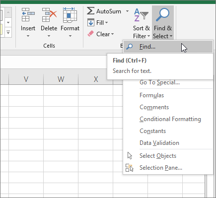
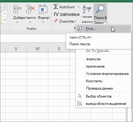
To find something, press Ctrl+F, or go to Home > Editing > Find & Select > Find.
Note: In the following example, we’ve clicked the Options >> button to show the entire Find dialog. By default, it will display with Options hidden.

-
In the Find what: box, type the text or numbers you want to find, or click the arrow in the Find what: box, and then select a recent search item from the list.
Tips: You can use wildcard characters — question mark (?), asterisk (*), tilde (~) — in your search criteria.
-
Use the question mark (?) to find any single character — for example, s?t finds «sat» and «set».
-
Use the asterisk (*) to find any number of characters — for example, s*d finds «sad» and «started».
-
Use the tilde (~) followed by ?, *, or ~ to find question marks, asterisks, or other tilde characters — for example, fy91~? finds «fy91?».
-
-
Click Find All or Find Next to run your search.
Tip: When you click Find All, every occurrence of the criteria that you are searching for will be listed, and clicking a specific occurrence in the list will select its cell. You can sort the results of a Find All search by clicking a column heading.
-
Click Options>> to further define your search if needed:
-
Within: To search for data in a worksheet or in an entire workbook, select Sheet or Workbook.
-
Search: You can choose to search either By Rows (default), or By Columns.
-
Look in: To search for data with specific details, in the box, click Formulas, Values, Notes, or Comments.
Note: Formulas, Values, Notes and Comments are only available on the Find tab; only Formulas are available on the Replace tab.
-
Match case — Check this if you want to search for case-sensitive data.
-
Match entire cell contents — Check this if you want to search for cells that contain just the characters that you typed in the Find what: box.
-
-
If you want to search for text or numbers with specific formatting, click Format, and then make your selections in the Find Format dialog box.
Tip: If you want to find cells that just match a specific format, you can delete any criteria in the Find what box, and then select a specific cell format as an example. Click the arrow next to Format, click Choose Format From Cell, and then click the cell that has the formatting that you want to search for.
Replace
To replace text or numbers, press Ctrl+H, or go to Home > Editing > Find & Select > Replace.
Note: In the following example, we’ve clicked the Options >> button to show the entire Find dialog. By default, it will display with Options hidden.

-
In the Find what: box, type the text or numbers you want to find, or click the arrow in the Find what: box, and then select a recent search item from the list.
Tips: You can use wildcard characters — question mark (?), asterisk (*), tilde (~) — in your search criteria.
-
Use the question mark (?) to find any single character — for example, s?t finds «sat» and «set».
-
Use the asterisk (*) to find any number of characters — for example, s*d finds «sad» and «started».
-
Use the tilde (~) followed by ?, *, or ~ to find question marks, asterisks, or other tilde characters — for example, fy91~? finds «fy91?».
-
-
In the Replace with: box, enter the text or numbers you want to use to replace the search text.
-
Click Replace All or Replace.
Tip: When you click Replace All, every occurrence of the criteria that you are searching for will be replaced, while Replace will update one occurrence at a time.
-
Click Options>> to further define your search if needed:
-
Within: To search for data in a worksheet or in an entire workbook, select Sheet or Workbook.
-
Search: You can choose to search either By Rows (default), or By Columns.
-
Look in: To search for data with specific details, in the box, click Formulas, Values, Notes, or Comments.
Note: Formulas, Values, Notes and Comments are only available on the Find tab; only Formulas are available on the Replace tab.
-
Match case — Check this if you want to search for case-sensitive data.
-
Match entire cell contents — Check this if you want to search for cells that contain just the characters that you typed in the Find what: box.
-
-
If you want to search for text or numbers with specific formatting, click Format, and then make your selections in the Find Format dialog box.
Tip: If you want to find cells that just match a specific format, you can delete any criteria in the Find what box, and then select a specific cell format as an example. Click the arrow next to Format, click Choose Format From Cell, and then click the cell that has the formatting that you want to search for.
There are two distinct methods for finding or replacing text or numbers on the Mac. The first is to use the Find & Replace dialog. The second is to use the Search bar in the ribbon.
Find & Replace dialog
Search bar and options

-
Press Ctrl+F or go to Home > Find & Select > Find.
-
In Find what: type the text or numbers you want to find.
-
Select Find Next to run your search.
-
You can further define your search:
-
Within: To search for data in a worksheet or in an entire workbook, select Sheet or Workbook.
-
Search: You can choose to search either By Rows (default), or By Columns.
-
Look in: To search for data with specific details, in the box, click Formulas, Values, Notes, or Comments.
-
Match case — Check this if you want to search for case-sensitive data.
-
Match entire cell contents — Check this if you want to search for cells that contain just the characters that you typed in the Find what: box.
-
Tips: You can use wildcard characters — question mark (?), asterisk (*), tilde (~) — in your search criteria.
-
Use the question mark (?) to find any single character — for example, s?t finds «sat» and «set».
-
Use the asterisk (*) to find any number of characters — for example, s*d finds «sad» and «started».
-
Use the tilde (~) followed by ?, *, or ~ to find question marks, asterisks, or other tilde characters — for example, fy91~? finds «fy91?».

-
Press Ctrl+F or go to Home > Find & Select > Find.
-
In Find what: type the text or numbers you want to find.
-
Select Find All to run your search for all occurrences.

Note: The dialog box expands to show a list of all the cells that contain the search term, and the total number of cells in which it appears.
-
Select any item in the list to highlight the corresponding cell in your worksheet.
Note: You can edit the contents of the highlighted cell.

-
Press Ctrl+H or go to Home > Find & Select > Replace.
-
In Find what, type the text or numbers you want to find.
-
You can further define your search:
-
Within: To search for data in a worksheet or in an entire workbook, select Sheet or Workbook.
-
Search: You can choose to search either By Rows (default), or By Columns.
-
Match case — Check this if you want to search for case-sensitive data.
-
Match entire cell contents — Check this if you want to search for cells that contain just the characters that you typed in the Find what: box.
Tips: You can use wildcard characters — question mark (?), asterisk (*), tilde (~) — in your search criteria.
-
Use the question mark (?) to find any single character — for example, s?t finds «sat» and «set».
-
Use the asterisk (*) to find any number of characters — for example, s*d finds «sad» and «started».
-
Use the tilde (~) followed by ?, *, or ~ to find question marks, asterisks, or other tilde characters — for example, fy91~? finds «fy91?».
-
-
-
In the Replace with box, enter the text or numbers you want to use to replace the search text.
-
Select Replace or Replace All.
Tips:
-
When you select Replace All, every occurrence of the criteria that you are searching for is replaced.
-
When you select Replace, you can replace one instance at a time by selecting Next to highlight the next instance.
-
-
Select any cell to search the entire sheet or select a specific range of cells to search.
-
Press Command + F or select the magnifying glass to expand the Search bar and type the text or number you want to find in the search field.
Tips: You can use wildcard characters — question mark (?), asterisk (*), tilde (~) — in your search criteria.
-
Use the question mark (?) to find any single character — for example, s?t finds «sat» and «set».
-
Use the asterisk (*) to find any number of characters — for example, s*d finds «sad» and «started».
-
Use the tilde (~) followed by ?, *, or ~ to find question marks, asterisks, or other tilde characters — for example, fy91~? finds «fy91?».
-
-
Press return.
Notes:
-
To find the next instance of the item you are searching for, press return again or use the Find dialog box and select Find Next.
-
To specify additional search options, select the magnifying glass and select Search in Sheet or Search in Workbook. You can also select the Advanced option, which launches the Find dialog.
Tip: You can cancel a search in progress by pressing ESC.
-
Find
To find something, press Ctrl+F, or go to Home > Editing > Find & Select > Find.
Note: In the following example, we’ve clicked > Search Options to show the entire Find dialog. By default, it will display with Search Options hidden.

-
In the Find what: box, type the text or numbers you want to find.
Tips: You can use wildcard characters — question mark (?), asterisk (*), tilde (~) — in your search criteria.
-
Use the question mark (?) to find any single character — for example, s?t finds «sat» and «set».
-
Use the asterisk (*) to find any number of characters — for example, s*d finds «sad» and «started».
-
Use the tilde (~) followed by ?, *, or ~ to find question marks, asterisks, or other tilde characters — for example, fy91~? finds «fy91?».
-
-
Click Find Next or Find All to run your search.
Tip: When you click Find All, every occurrence of the criteria that you are searching for will be listed, and clicking a specific occurrence in the list will select its cell. You can sort the results of a Find All search by clicking a column heading.
-
Click > Search Options to further define your search if needed:
-
Within: To search for data within a certain selection, choose Selection. To search for data in a worksheet or in an entire workbook, select Sheet or Workbook.
-
Direction: You can choose to search either Down (default), or Up.
-
Match case — Check this if you want to search for case-sensitive data.
-
Match entire cell contents — Check this if you want to search for cells that contain just the characters that you typed in the Find what box.
-
Replace
To replace text or numbers, press Ctrl+H, or go to Home > Editing > Find & Select > Replace.
Note: In the following example, we’ve clicked > Search Options to show the entire Find dialog. By default, it will display with Search Options hidden.

-
In the Find what: box, type the text or numbers you want to find.
Tips: You can use wildcard characters — question mark (?), asterisk (*), tilde (~) — in your search criteria.
-
Use the question mark (?) to find any single character — for example, s?t finds «sat» and «set».
-
Use the asterisk (*) to find any number of characters — for example, s*d finds «sad» and «started».
-
Use the tilde (~) followed by ?, *, or ~ to find question marks, asterisks, or other tilde characters — for example, fy91~? finds «fy91?».
-
-
In the Replace with: box, enter the text or numbers you want to use to replace the search text.
-
Click Replace or Replace All.
Tip: When you click Replace All, every occurrence of the criteria that you are searching for will be replaced, while Replace will update one occurrence at a time.
-
Click > Search Options to further define your search if needed:
-
Within: To search for data within a certain selection, choose Selection. To search for data in a worksheet or in an entire workbook, select Sheet or Workbook.
-
Direction: You can choose to search either Down (default), or Up.
-
Match case — Check this if you want to search for case-sensitive data.
-
Match entire cell contents — Check this if you want to search for cells that contain just the characters that you typed in the Find what box.
-
Need more help?
You can always ask an expert in the Excel Tech Community or get support in the Answers community.
Recommended articles
Merge and unmerge cells
REPLACE, REPLACEB functions
Apply data validation to cells
Функция НАЙТИ (FIND) в Excel используется для поиска текстового значения внутри строчки с текстом и указать порядковый номер буквы с которого начинается искомое слово в найденной строке.
Содержание
- Что возвращает функция
- Синтаксис
- Аргументы функции
- Дополнительная информация
- Примеры использования функции НАЙТИ в Excel
- Пример 1. Ищем слово в текстовой строке (с начала строки)
- Пример 2. Ищем слово в текстовой строке (с заданным порядковым номером старта поиска)
- Пример 3. Поиск текстового значения внутри текстовой строки с дублированным искомым значением
Что возвращает функция
Возвращает числовое значение, обозначающее стартовую позицию текстовой строчки внутри другой текстовой строчки.
Синтаксис
=FIND(find_text, within_text, [start_num]) — английская версия
=НАЙТИ(искомый_текст;просматриваемый_текст;[нач_позиция]) — русская версия
Аргументы функции
- find_text (искомый_текст) — текст или строка которую вы хотите найти в рамках другой строки;
- within_text (просматриваемый_текст) — текст, внутри которого вы хотите найти аргумент find_text (искомый_текст);
- [start_num] ([нач_позиция]) — число, отображающее позицию, с которой вы хотите начать поиск. Если аргумент не указать, то поиск начнется сначала.
Дополнительная информация
- Если стартовое число не указано, то функция начинает поиск искомого текста с начала строки;
- Функция НАЙТИ чувствительна к регистру. Если вы хотите сделать поиск без учета регистра, используйте функцию SEARCH в Excel;
- Функция не учитывает подстановочные знаки при поиске. Если вы хотите использовать подстановочные знаки для поиска, используйте функцию SEARCH в Excel;
- Функция каждый раз возвращает ошибку, когда не находит искомый текст в заданной строке.
Примеры использования функции НАЙТИ в Excel
Пример 1. Ищем слово в текстовой строке (с начала строки)

На примере выше мы ищем слово «Доброе» в словосочетании «Доброе Утро». По результатам поиска, функция выдает число «1», которое обозначает, что слово «Доброе» начинается с первой по очереди буквы в, заданной в качестве области поиска, текстовой строке.
Больше лайфхаков в нашем Telegram Подписаться
Обратите внимание, что так как функция НАЙТИ в Excel чувствительна к регистру, вы не сможете найти слово «доброе» в словосочетании «Доброе утро», так как оно написано с маленькой буквы. Для того, чтобы осуществить поиска без учета регистра следует пользоваться функцией SEARCH.
Пример 2. Ищем слово в текстовой строке (с заданным порядковым номером старта поиска)
Третий аргумент функции НАЙТИ указывает позицию, с которой функция начинает поиск искомого значения. На примере выше функция возвращает число «1» когда мы начинаем поиск слова «Доброе» в словосочетании «Доброе утро» с начала текстовой строки. Но если мы зададим аргумент функции start_num (нач_позиция) со значением «2», то функция выдаст ошибку, так как начиная поиск со второй буквы текстовой строки, она не может ничего найти.
Если вы не укажете номер позиции, с которой функции следует начинать поиск искомого аргумента, то Excel по умолчанию начнет поиск с самого начала текстовой строки.
Пример 3. Поиск текстового значения внутри текстовой строки с дублированным искомым значением
На примере выше мы ищем слово «Доброе» в словосочетании «Доброе Доброе утро». Когда мы начинаем поиск слова «Доброе» с начала текстовой строки, то функция выдает число «1», так как первое слово «Доброе» начинается с первой буквы в словосочетании «Доброе Доброе утро».
Но, если мы укажем в качестве аргумента start_num (нач_позиция) число «2» и попросим функцию начать поиск со второй буквы в заданной текстовой строке, то функция выдаст число «6», так как Excel находит искомое слово «Доброе» начиная со второй буквы словосочетания «Доброе Доброе утро» только на 6 позиции.
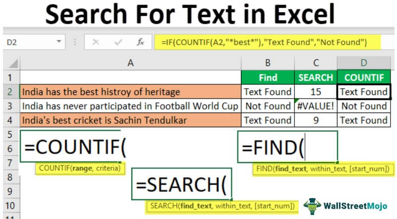
When working with Excel, we see so many peculiar situations. One of those situations is searching for the particular text in the cell. The first thing that comes to mind when we say we want to search for a specific text in the worksheet is the “Find and Replace” method in Excel, which is the most popular one. But Ctrl + F can find the text you are looking for but cannot go beyond that. So, for example, if the cell contains certain words, you may want the result in the next cell as “TRUE” or “FALSE.” So, Ctrl + F stops there.
Table of contents
- How to Search For Text in Excel?
- Which Formula Can Tell Us A Cell Contains Specific Text?
- Alternatives to FIND Function
- Alternative #1 – Excel Search Function
- Alternative #2 – Excel Countif Function
- Highlight the Cell which has Particular Text Value
- Recommended Articles
Here, we will take you through the formulas to search for the particular text in the cell value and arrive at the result.
You can download this Search For Text Excel Template here – Search For Text Excel Template
Which Formula Can Tell Us A Cell Contains Specific Text?
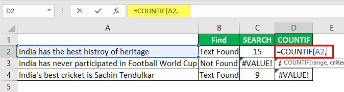
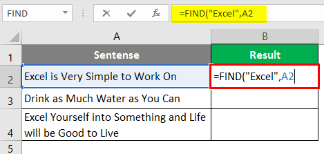
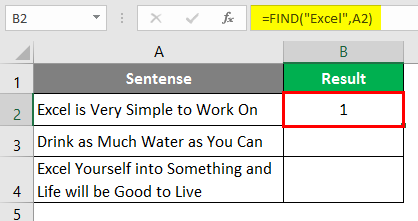
It is a question we have seen many times in Excel forums. The first formula that came to mind was the “FIND” function.
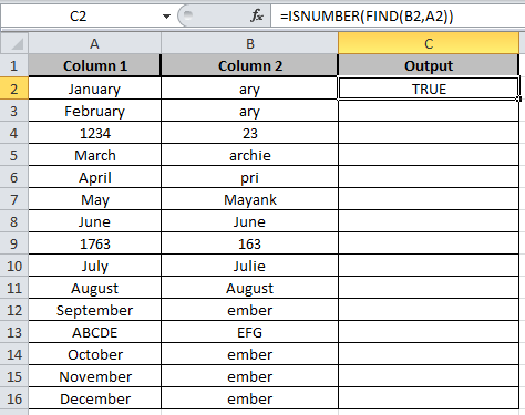
The FIND function can return the position of the supplied text values in the string. So, if the FIND method returns any number, then we can consider the cell as it has the text or else not.
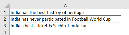
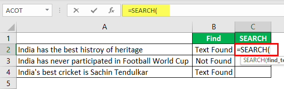
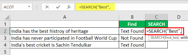
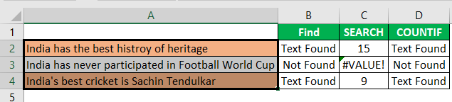
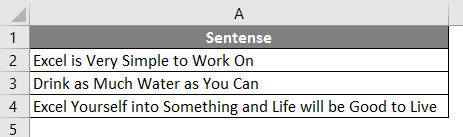
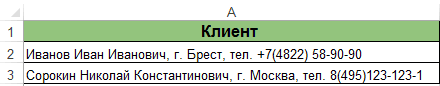
- For example, look at the below data.

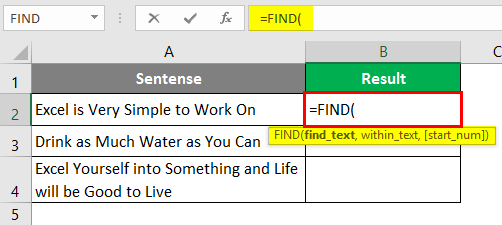
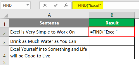
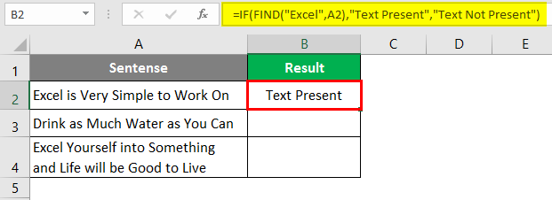
- In the above data, we have three sentences in three different rows. Now in each cell, we need to search for the text “Best.” So, apply the FIND function.

- The “find_text” argument mentions the text we need to find.

- For the “within_text,” select the full sentence, i.e., cell reference.

- The last parameter is not required to close the bracket and press the “Enter” key.

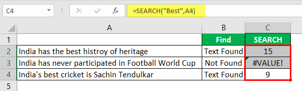
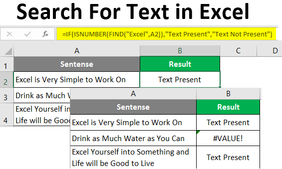
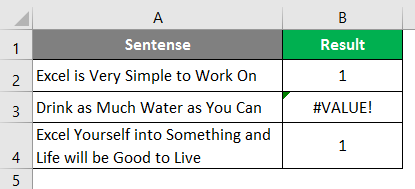
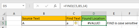
So, in two sentences, we have the word “best.” We can see the error value of #VALUE! in cell B2, which shows that cell A2 does not have the text value “best.”
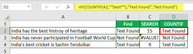
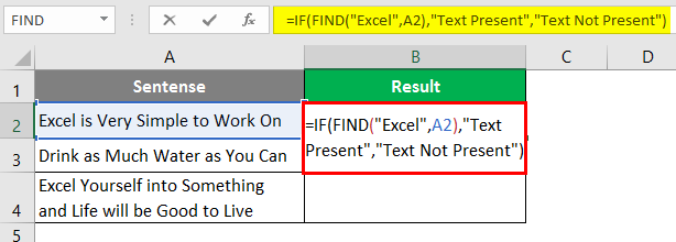
- Instead of numbers, we can also enter the result in our own words. For this, we need to use the IF condition.


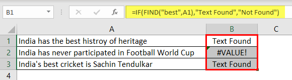
So, in the IF condition, we have supplied the result as “Text Found” if the value “best” is found. Otherwise, we have provided the result as “Not Found.”
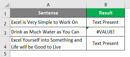
But, here we have a problem, even though we have supplied the result as “Not Found,” if the text is still not found, we are getting the error value as #VALUE!.
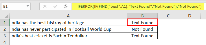
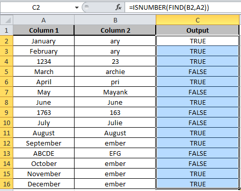
So, nobody wants to have an error value in their Excel sheet. Therefore, we must enclose the formula with the ISNUMERIC function to overcome this error value.

The ISNUMERIC function evaluates whether the FIND function returns the number or not. If the FIND function returns the number, it will supply TRUE to the IF condition or else FALSE condition. Based on the result provided by the ISNUMERIC function, the IF condition will return the result accordingly.
We can also use the IFERROR function in excelThe IFERROR function in Excel checks a formula (or a cell) for errors and returns a specified value in place of the error.read more to deal with error values instead of ISNUMERIC. For example, the below formula will also return “Not Found” if the FIND function returns the error value.
Alternatives to FIND Function
Alternative #1 – Excel Search Function
Instead of the FIND function, we can also use the SEARCH function in excelSearch function gives the position of a substring in a given string when we give a parameter of the position to search from. As a result, this formula requires three arguments. The first is the substring, the second is the string itself, and the last is the position to start the search.read more to search the particular text in the string. The syntax of the SEARCH function is the same as the FIND function.
Supply the “find_text” as “Best.”
The “within_text” is our cell reference.
Even the SEARCH function returns an error value as #VALUE! If the finding text “best” is not found. As we have seen above, we need to enclose the formula with ISNUMERIC or IFERROR functions.
Alternative #2 – Excel Countif Function
Another way to search for a particular text is using the COUNTIF functionThe COUNTIF function in Excel counts the number of cells within a range based on pre-defined criteria. It is used to count cells that include dates, numbers, or text. For example, COUNTIF(A1:A10,”Trump”) will count the number of cells within the range A1:A10 that contain the text “Trump”
read more. This function works without any error.
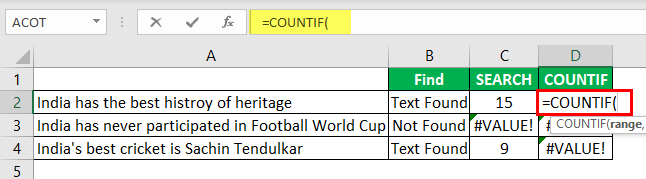
In the range, the argument selects the cell reference.
In the criteria column, we need to use a wildcard in excelIn Excel, wildcards are the three special characters asterisk, question mark, and tilde. Asterisk denotes multiple characters, a question mark denotes a single character, and a tilde denotes the identification of a wild card character.read more because we are just finding the part of the string value, so enclose the word “best” with an asterisk (*) wildcard.
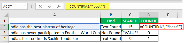
This formula will return the word “best” count in the selected cell value. Since we have only one “best” value, we will get only 1 as the count.
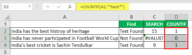
We can apply only the IF condition to get the result without error.
Highlight the Cell which has a Particular Text Value
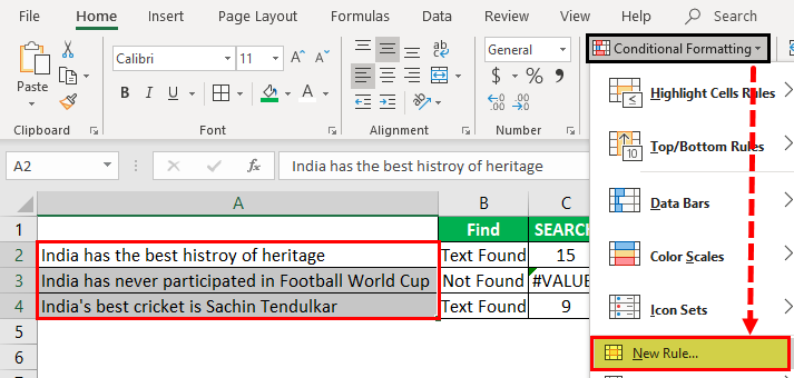
If you are not a fan of formulas, you can highlight the cell with a particular word. For example, to highlight the cell with the word “best,” we need to use conditional formatting in excelConditional formatting is a technique in Excel that allows us to format cells in a worksheet based on certain conditions. It can be found in the styles section of the Home tab.read more.
First, select the data cells and click “Conditional Formatting” > “New Rule.”
Under “New Rule,” select the “Format only cells that contain” option.
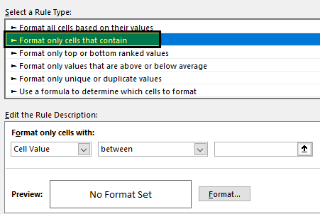
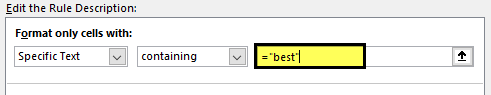
From the first dropdown, select “Specific Text.”

The formula section enters the text we search for in double quotes with the equal sign. =’best.’
Then, click on “FORMAT” and choose the formatting style.
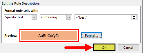
Click on “OK.” It will highlight all the cells which have the word “best.”
Using various techniques, we can search the particular text in Excel.
Recommended Articles
This article is a guide to Search For Text in Excel. Here, we discuss the top three methods to search the cell value for a specific text and arrive at the result with practical examples and a downloadable Excel template. You may learn more about Excel from the following articles: –
- Find Links in Excel
- Using Find and Select in Excel
- Search Box in Excel
Содержание
- FIND, FINDB functions
- Description
- Syntax
- Remarks
- Examples
- Check if a cell contains text (case-insensitive)
- Find cells that contain text
- Check if a cell has any text in it
- Check if a cell matches specific text
- Check if part of a cell matches specific text
- Find or replace text and numbers on a worksheet
- Replace
- Search For Text in Excel
- Searching For Text in Excel
- How to Search Text in Excel?
- Example #1 – Using Find Function
- Example #2 – Using SEARCH Function
- Things to Remember About Search For Text in Excel
- Recommended Articles
FIND, FINDB functions
This article describes the formula syntax and usage of the FIND and FINDB functions in Microsoft Excel.
Description
FIND and FINDB locate one text string within a second text string, and return the number of the starting position of the first text string from the first character of the second text string.
These functions may not be available in all languages.
FIND is intended for use with languages that use the single-byte character set (SBCS), whereas FINDB is intended for use with languages that use the double-byte character set (DBCS). The default language setting on your computer affects the return value in the following way:
FIND always counts each character, whether single-byte or double-byte, as 1, no matter what the default language setting is.
FINDB counts each double-byte character as 2 when you have enabled the editing of a language that supports DBCS and then set it as the default language. Otherwise, FINDB counts each character as 1.
The languages that support DBCS include Japanese, Chinese (Simplified), Chinese (Traditional), and Korean.
Syntax
FIND(find_text, within_text, [start_num])
FINDB(find_text, within_text, [start_num])
The FIND and FINDB function syntax has the following arguments:
Find_text Required. The text you want to find.
Within_text Required. The text containing the text you want to find.
Start_num Optional. Specifies the character at which to start the search. The first character in within_text is character number 1. If you omit start_num, it is assumed to be 1.
FIND and FINDB are case sensitive and don’t allow wildcard characters. If you don’t want to do a case sensitive search or use wildcard characters, you can use SEARCH and SEARCHB.
If find_text is «» (empty text), FIND matches the first character in the search string (that is, the character numbered start_num or 1).
Find_text cannot contain any wildcard characters.
If find_text does not appear in within_text, FIND and FINDB return the #VALUE! error value.
If start_num is not greater than zero, FIND and FINDB return the #VALUE! error value.
If start_num is greater than the length of within_text, FIND and FINDB return the #VALUE! error value.
Use start_num to skip a specified number of characters. Using FIND as an example, suppose you are working with the text string «AYF0093.YoungMensApparel». To find the number of the first «Y» in the descriptive part of the text string, set start_num equal to 8 so that the serial-number portion of the text is not searched. FIND begins with character 8, finds find_text at the next character, and returns the number 9. FIND always returns the number of characters from the start of within_text, counting the characters you skip if start_num is greater than 1.
Examples
Copy the example data in the following table, and paste it in cell A1 of a new Excel worksheet. For formulas to show results, select them, press F2, and then press Enter. If you need to, you can adjust the column widths to see all the data.
Источник
Check if a cell contains text (case-insensitive)
Let’s say you want to ensure that a column contains text, not numbers. Or, perhapsyou want to find all orders that correspond to a specific salesperson. If you have no concern for upper- or lowercase text, there are several ways to check if a cell contains text.
You can also use a filter to find text. For more information, see Filter data.
Find cells that contain text
Follow these steps to locate cells containing specific text:
Select the range of cells that you want to search.
To search the entire worksheet, click any cell.
On the Home tab, in the Editing group, click Find & Select, and then click Find.
In the Find what box, enter the text—or numbers—that you need to find. Or, choose a recent search from the Find what drop-down box.
Note: You can use wildcard characters in your search criteria.
To specify a format for your search, click Format and make your selections in the Find Format popup window.
Click Options to further define your search. For example, you can search for all of the cells that contain the same kind of data, such as formulas.
In the Within box, you can select Sheet or Workbook to search a worksheet or an entire workbook.
Click Find All or Find Next.
Find All lists every occurrence of the item that you need to find, and allows you to make a cell active by selecting a specific occurrence. You can sort the results of a Find All search by clicking a header.
Note: To cancel a search in progress, press ESC.
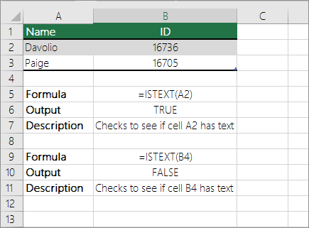
Check if a cell has any text in it
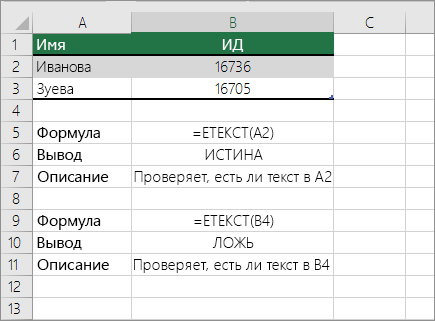
To do this task, use the ISTEXT function.
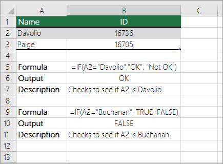
Check if a cell matches specific text
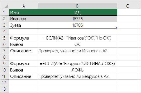
Use the IF function to return results for the condition that you specify.
Check if part of a cell matches specific text
To do this task, use the IF, SEARCH, and ISNUMBER functions.
Note: The SEARCH function is case-insensitive.
Источник
Find or replace text and numbers on a worksheet
Use the Find and Replace features in Excel to search for something in your workbook, such as a particular number or text string. You can either locate the search item for reference, or you can replace it with something else. You can include wildcard characters such as question marks, tildes, and asterisks, or numbers in your search terms. You can search by rows and columns, search within comments or values, and search within worksheets or entire workbooks.
Tip: You can also use formulas to replace text. Check out the SUBSTITUTE function or REPLACE, REPLACEB functions to learn more.
To find something, press Ctrl+F, or go to Home > Editing > Find & Select > Find.
Note: In the following example, we’ve clicked the Options >> button to show the entire Find dialog. By default, it will display with Options hidden.
In the Find what: box, type the text or numbers you want to find, or click the arrow in the Find what: box, and then select a recent search item from the list.
Tips: You can use wildcard characters — question mark ( ?), asterisk ( *), tilde (
) — in your search criteria.
Use the question mark (?) to find any single character — for example, s?t finds «sat» and «set».
Use the asterisk (*) to find any number of characters — for example, s*d finds «sad» and «started».
) followed by ?, *, or
to find question marks, asterisks, or other tilde characters — for example, fy91
Click Find All or Find Next to run your search.
Tip: When you click Find All, every occurrence of the criteria that you are searching for will be listed, and clicking a specific occurrence in the list will select its cell. You can sort the results of a Find All search by clicking a column heading.
Click Options>> to further define your search if needed:
Within: To search for data in a worksheet or in an entire workbook, select Sheet or Workbook.
Search: You can choose to search either By Rows (default), or By Columns.
Look in: To search for data with specific details, in the box, click Formulas, Values, Notes, or Comments.
Note: Formulas, Values, Notes and Comments are only available on the Find tab; only Formulas are available on the Replace tab.
Match case — Check this if you want to search for case-sensitive data.
Match entire cell contents — Check this if you want to search for cells that contain just the characters that you typed in the Find what: box.
If you want to search for text or numbers with specific formatting, click Format, and then make your selections in the Find Format dialog box.
Tip: If you want to find cells that just match a specific format, you can delete any criteria in the Find what box, and then select a specific cell format as an example. Click the arrow next to Format, click Choose Format From Cell, and then click the cell that has the formatting that you want to search for.
Replace
To replace text or numbers, press Ctrl+H, or go to Home > Editing > Find & Select > Replace.
Note: In the following example, we’ve clicked the Options >> button to show the entire Find dialog. By default, it will display with Options hidden.
In the Find what: box, type the text or numbers you want to find, or click the arrow in the Find what: box, and then select a recent search item from the list.
Tips: You can use wildcard characters — question mark ( ?), asterisk ( *), tilde (
) — in your search criteria.
Use the question mark (?) to find any single character — for example, s?t finds «sat» and «set».
Use the asterisk (*) to find any number of characters — for example, s*d finds «sad» and «started».
) followed by ?, *, or
to find question marks, asterisks, or other tilde characters — for example, fy91
In the Replace with: box, enter the text or numbers you want to use to replace the search text.
Click Replace All or Replace.
Tip: When you click Replace All, every occurrence of the criteria that you are searching for will be replaced, while Replace will update one occurrence at a time.
Click Options>> to further define your search if needed:
Within: To search for data in a worksheet or in an entire workbook, select Sheet or Workbook.
Search: You can choose to search either By Rows (default), or By Columns.
Look in: To search for data with specific details, in the box, click Formulas, Values, Notes, or Comments.
Note: Formulas, Values, Notes and Comments are only available on the Find tab; only Formulas are available on the Replace tab.
Match case — Check this if you want to search for case-sensitive data.
Match entire cell contents — Check this if you want to search for cells that contain just the characters that you typed in the Find what: box.
If you want to search for text or numbers with specific formatting, click Format, and then make your selections in the Find Format dialog box.
Tip: If you want to find cells that just match a specific format, you can delete any criteria in the Find what box, and then select a specific cell format as an example. Click the arrow next to Format, click Choose Format From Cell, and then click the cell that has the formatting that you want to search for.
There are two distinct methods for finding or replacing text or numbers on the Mac. The first is to use the Find & Replace dialog. The second is to use the Search bar in the ribbon.
Источник
Search For Text in Excel
Excel Search For Text (Table of Contents)
Searching For Text in Excel
In excel, you might have seen situations where you want to extract the text present at a specific position in an entire string using text formulae such as LEFT, RIGHT, MID, etc. You can also use SEARCH and FIND functions in combination to find the text substring from a given string. However, when you are not interested in finding out the substring, but you want to find out whether a particular string is present in a given cell or not, not all of these formulae will work. In this article, we will go through some of the formulae and/or functions in Excel, which will allow you to check whether or not a particular string is present in a given cell.
Excel functions, formula, charts, formatting creating excel dashboard & others
How to Search Text in Excel?
Search For Text in Excel is very simple and easy. Let’s understand how to Search Text in Excel with some examples.
Example #1 – Using Find Function
Let’s use the FIND function to find if a specific string is present in a cell or not. Suppose you have data as shown below.
As we are trying to find whether a specific text is present in a given string or not, we have a function called FIND to deal with it on an initial level. This function returns a position of a substring in a text cell. Therefore, we can say that if the FIND function returns any numeric value, then the substring is present in the text else not.
Step 1: In cell B1, start typing =FIND; you will be able to access the function itself.
Step 2: The FIND function needs at least two arguments: the string you want to search and the cell within which you want to search. Let’s use “Excel” as the first argument for the FIND function, which specifies find_text from the formula.
Step 3: We want to find whether “Excel” is present in cell A2 under a given worksheet. Therefore, choose A2 as the next argument to FIND function.
We are going to ignore the start_num argument as it is an optional argument.
Step 4: Close the parentheses to complete the formula and press Enter Key.
If you can see, this function just returned the position where the word “Excel” is present in the current cell (i.e. cell A2).
Step 5: Drag the formula to see the position where Excel belongs under cell A3 and A4.
You can see in the screenshot above that the mentioned string is present in two cells (A2 and A3). In cell B3 the word is not present; hence the formula is providing the #VALUE! error. This, however, doesn’t always provide a clearer picture. I mean, someone might not be good enough in excel to understand the fact that 1 appearing in cell B2 is nothing but the position of the word “Excel” in string occupied in cell A2.
Step 6: In order to get a customized result under column B, use the IF function and apply FIND under it. Once you use FIND under IF as a condition, you need to provide two possible outputs. One of the condition is TRUE, the other if the condition is FALSE. Press Enter after editing the formula with IF condition.
After using the above formula, the output is shown below.
Step 7: Drag the formula from cell B2 until cell B4.
Now, we have used IF and FIND in combinations; the cell with no string still gives #VALUE! error. Let’s try to remove this error with the help of the ISNUMBER function.
ISNUMBER function checks if the output is number or not. If the output is a number, it will give TRUE as a value; if not a number, then it will give FALSE as a value if we use this function in combination with IF and FIND, IF function will give the output based on the values (either TRUE or FALSE) provided by ISNUMBER function.
Step 8: Use ISNUMBER in the formula we used above in step 6 and step 7. Press Enter Key after editing the formula under cell B2.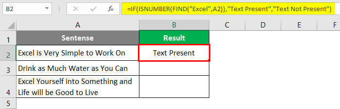
Step 9: Drag the formula across cell B2 to B4.
Clearly the #VALUE! error present in previous steps was nullified due to the ISNUMBER function.
Example #2 – Using SEARCH Function
On similar lines to that of the FIND function, the SEARCH function in excel also allows you to search whether the given substring is present within a text or not. You can use it on the same lines; we have used the FIND function and its combination with IF and ISNUMBER.
SEARCH function also searches the specific string inside the given text and returns the text’s position.
I will directly show you the final formula for finding if a string is present or not in Excel using the combination of SEARCH, IF and ISNUMBER function. You can follow steps 1 to 9, all in the same sequence from the previous example. The only change will be to replace FIND with the SEARCH function.
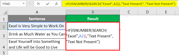
Use the following formula in cell B2 of the sheet “Example 2”, and press Enter Key to see the output (We have the same data as used in the previous example) =IF(ISNUMBER(SEARCH(“Excel”,A1)),”Text Present”, “Text Not Present”) Once you press Enter Key, you’ll see an output the same as in the previous example.
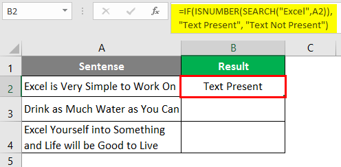
Drag the formula across the cells B2 to B4 to see the final output.
In cell A2 and A4, the word “Excel” is present; hence it has output as “Text Present”. However, in cell A3, the word “Excel” is not present; therefore, it has output as “Text Not Present”.
This is from this article. Let’s wrap the things with some things to be remembered.
Things to Remember About Search For Text in Excel
- These functions are used to check whether the given string is present in the text provided. In case you need to extract the substring from any string, you need to use the LEFT, RIGHT, MID functions altogether.
- ISNUMBER function is used in combination so that you are not getting any #VALUE! error if the string is not present in the text provided.
Recommended Articles
This is a guide to Search For Text in Excel. Here we discuss How to Search Text in Excel along with practical examples and a downloadable excel template. You can also go through our other suggested articles –
Источник
Excel FIND Function (Example + Video)
When to use Excel FIND Function
Excel FIND function can be used when you want to locate a text string within another text string and find its position.
What it Returns
It returns a number that represents the starting position of the string you are finding in another string.
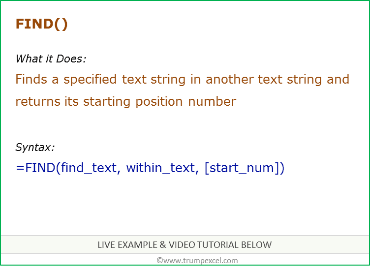
Syntax
=FIND(find_text, within_text, [start_num])
Input Arguments
- find_text – the text or string that you need to find.
- within_text – the text within which you want to find the find_text argument.
- [start_num] – a number that represents the position from which you want the search to begin. If you omit it, it starts from the beginning.
Additional Notes
- If the start number is not specified, then it starts looking from the beginning of the string.
- Excel FIND function is case-sensitive. If you want to do a case-insensitive search, use Excel SEARCH function.
- Excel FIND function cannot handle wildcard characters. If you want to use wildcard characters, use the Excel SEARCH function.
- It returns a #VALUE! error if the searched string is not found in the text.
Excel FIND Function – Examples
Here are four examples of using Excel FIND function:
Searching for a Word in a Text String (from the beginning)
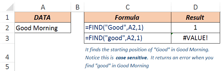
In the above example, when you look for the word Good in the text Good Morning, it returns 1, which is the position of the starting point of the searched word.
Note that Excel FIND function is case-sensitive. When you use good instead of Good, it returns a #VALUE! error.
If you are looking for a case-insensitive search, use Excel SEARCH function.
Finding a Word in a Text String (with a specified beginning)
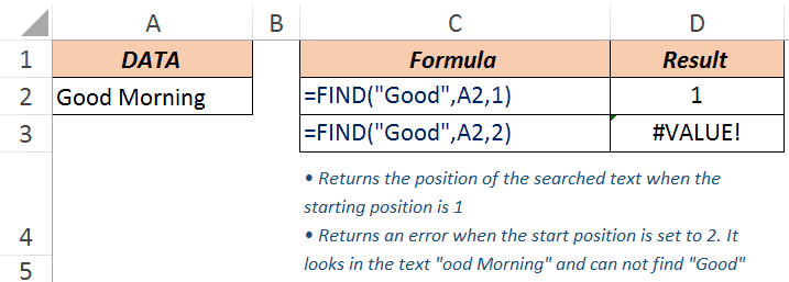
The third argument in the FIND function is the position within the text from where you want to start the search. In the example above, the function returns 1 when you search for the text Good in Good Morning and the starting position is 1.
However, it returns an error when you make it start at 2. Hence, it looks for the text Good in ood Morning. Since it can not find it, it returns an error.
Note: If you skip the last argument and don’t provide the starting position, by default it takes it as 1.
When there are Multiple Occurrence of the Searched Text
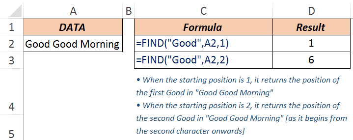
Excel FIND function starts looking in the specified text from the specified position. In the above example, when you look for the text Good in Good Good Morning with the starting position as 1, it returns 1, as it finds it at the beginning.
When you start the search from the second character onwards, it returns 6, as it finds the matching text at the sixth position.
Extracting Everything to the Left a Specified Character/String
Suppose you have the email ids do some superheroes as shown below and you want to extract only the username part (which would be the characters before the @).
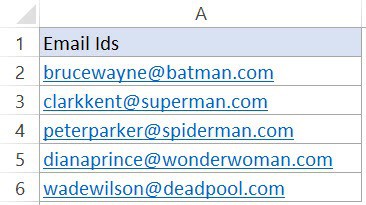
Below is the formula that will find the position of ‘@’ in each email id and extract all the characters to the left of it:
=LEFT(A2,FIND(“@”,A2,1)-1)

The FIND function in this formula gives the position of the ‘@’ character. The LEFT function that uses this position to extract the username.
For example, in the case of brucewayne@batman.com, the FIND function returns 11. LEFT function then uses FIND(“@”,A2,1)-1 as the second argument to get the username.
Note that 1 is subtracted from the value returned by the FIND function as we want to exclude the @ from the result of the LEFT function.
Excel FIND Function – VIDEO
Related Excel Functions:
- Excel LOWER Function.
- Excel UPPER Function.
- Excel PROPER Function.
- Excel REPLACE Function.
- Excel SEARCH Function.
- Excel SUBSTITUTE Function.
You May Also Like the Following Tutorials:
- How to Quickly Find and Remove Hyperlinks in Excel.
- How to Find Merged Cells in Excel.
- How to Find and Remove Duplicates in Excel.
- Using Find and Replace in Excel.
The SEARCH function returns the position (as a number) of one text string inside another. If there is more than one occurrence of the search string, SEARCH returns the position of the first occurrence. SEARCH is not case-sensitive but does support wildcards. Use the FIND function to perform a case-sensitive find. When SEARCH does not find anything, it returns a #VALUE! error. Note that when find_text is empty, SEARCH will return 1. This can cause a false positive when find_text is an empty cell.
Basic Example
The SEARCH function is designed to look inside a text string for a specific substring. If SEARCH finds the substring, it returns a position of the substring in the text as a number. If the substring is not found, SEARCH returns a #VALUE error. For example:
=SEARCH("p","apple") // returns 2
=SEARCH("z","apple") // returns #VALUE!
Note that text values entered directly into SEARCH must be enclosed in double-quotes («»).
TRUE or FALSE result
To force a TRUE or FALSE result, nest SEARCH inside the ISNUMBER function. ISNUMBER returns TRUE for numbers and FALSE for anything else. If SEARCH finds the substring, it returns the position as a number, and ISNUMBER returns TRUE:
=ISNUMBER(SEARCH("p","apple")) // returns TRUE
=ISNUMBER(SEARCH("z","apple")) // returns FALSE
If SEARCH doesn’t find the substring, it returns an error, and ISNUMBER returns FALSE.
Start number
The SEARCH function has an optional argument called start_num, that controls where SEARCH should begin looking for a substring. To find the first match of «the», you can omit start_num, which defaults to 1:
=SEARCH("the","The cat in the hat") // returns 1
To start searching at character 4, enter 4 for start_num:
=SEARCH("the","The cat in the hat",4) // returns 12
Wildcards
Although SEARCH is not case-sensitive, it does support wildcards (*?~). For example, the question mark (?) wildcard matches any one character. The formula below looks for a 3-character substring beginning with «x» and ending in «y»:
=ISNUMBER(SEARCH("x?z","xyz")) // TRUE
=ISNUMBER(SEARCH("x?z","xbz")) // TRUE
=ISNUMBER(SEARCH("x?z","xyy")) // FALSE
The asterisk (*) wildcard is not as useful in the SEARCH function because SEARCH already looks for a substring. For example, it might seem like the following formula will test for a value that ends with «z»:
=SEARCH("*z",text)However, because SEARCH automatically looks for a substring, the following formulas all return 1 as a result, even though the text in the first formula is the only text that ends with «z»:
=SEARCH("*z","XYZ") // returns 1
=SEARCH("*z","XYZXY") // returns 1
=SEARCH("*z","XYZXY123") // returns 1
=SEARCH("x*z","XYZXY123") // returns 1
However, it is possible to use the asterisk (*) wildcard like this:
=SEARCH("x*2*b","AAAXYZ123ABCZZZ") // returns 4
=SEARCH("x*2*b","NXYZ12563JKLB") // returns 2
Here we are looking for «x», «2», and «b» in that order, with any number of characters in between. Finally, use the tilde (~) as an escape character to indicate that the next character is a literal like this:
=SEARCH("~*","apple*") // returns 6
=SEARCH("~?","apple?") // returns 6
=SEARCH("~~","apple~") // returns 6
The above formulas use SEARCH to find a literal asterisk (*), question mark (?) , and tilde (~) in that order.
If cell contains
To return a custom result with the SEARCH function, use the IF function like this:
=IF(ISNUMBER(SEARCH(substring,A1)), "Yes", "No")
Instead of returning TRUE or FALSE, the formula above will return «Yes» if substring is found and «No» if not.
Notes
- SEARCH returns the position of the first find_text in within_text.
- Start_num is optional and defaults to 1.
- Use the FIND function for a case-sensitive search.
- SEARCH allows the wildcard characters question mark (?) and asterisk (*), in find_text.
- ? matches any single character and
- * matches any sequence of characters.
- To find a literal ? or *, use a tilde (~) before the character, i.e. ~* and ~?.

In this article, we will learn How to use the FIND function in Excel.
Find any text in Excel
In Excel, you need to find the position of a text. Either you can count manually watching closely each cell value. Excel doesn’t want you to do that and neither do we. For example finding the position of space character to divide values wherever space exists like separating first name and last name from the full name. So let’s see the FIND function syntax and an example to illustrate its use.
In the cell Jimmy Kimmel, Space character comes right after the y and before K. 6th is the occurrence of Space char in word starting from J.
FIND Function in Excel
FIND function just needs two arguments (third optional). Given a partial text or single character to find within a text value is done using the FIND function.
FIND function Syntax:
=FIND(find_text, within_text, [start_num])
Find_text : The character or set of characters you want to find in string.
Within_text : The text or cell reference in which you want to find the text
[start_num] : optional. The starting point of search.
Example :
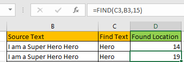
All of these might be confusing to understand. Let’s understand how to use the function using an example. Here Just to explain FIND function better, I have prepared this data.
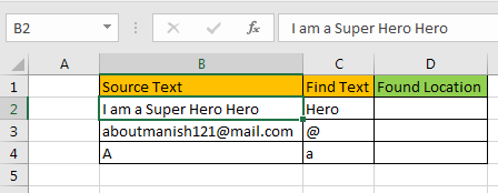
In Cell D2 to D4, I want to find the location of “Hero” in cell B2, “@” in cell B3 and “a” in B4, respectively.
I write this FIND formula in Cell D2 and drag it down to cell D4.
Use the Formula in D4 cell
And now i have the location of the given text:
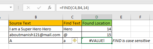
Find the Second, Third and Nth Occurrence of Given Characters in the Strings.
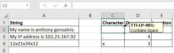
Here we have some strings in range A2:A4. In cell C2, C3, and C4 we have mentioned the characters that we want to search in the strings. In D2, D3, and D4 we have mentioned the occurrence of the character. In the adjacent cell I want to get the position of these occurrences of the characters.
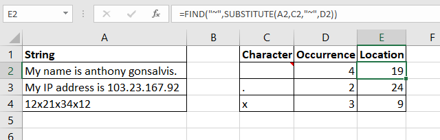
Write this formula in the cell E2 and drag down.
This returns the exact positions (19) of the mentioned occurrence (4) of the space character in the string.
How does it work?
The technique is quite simple. As we know the SUBSTITUTE function of Excel replaces the given occurrence of a text in string with the given text. We use this property.
So the formula works from inside.
SUBSTITUTE(A2,C2,»~»,D2): This part resolves to SUBSTITUTE(«My name is anthony gonsalvis.«
,» «,»~»,4). Which ultimately gives us the string «My name is anthony~gonsalvis.«
P.S. : the fourth occurrence of space is replaced with «~». I replaced space with «~» because I am sure that this character will not appear in the string by default. You can use any character that you are sure will not appear in the string. You can use the CHAR function to insert symbols.
Search substring in Excel
Here we have two columns. Substring in Column B and Given string in Column A.
Write the formula in the C2 cell.
Formula:
Explanation:
Find function takes the substring from the B2 cell of Column B and it then matches it with the given string in the A2 cell of Column A.
ISNUMBER checks if the string matches, it returns True else it returns False.
Copy the formula in other cells, select the cells taking the first cell where the formula is already applied, use shortcut key Ctrl + D.
As you can see the output in column C shows True and False representing whether substring is there or not.
Here are all the observational notes using the FIND function in Excel
Notes :
FIND returns the first found location by default.
If you want a second found location of text then provide start_num and it should be greater than first location of the text.
If the given text is not found, FIND formula will return #VALUE error.
FIND is case sensitive. If you need an case insentive function, use the SEARCH function.

FIND does not support wildcard characters. Use the SEARCH function if you need to use wildcards to find text in a string.
Hope this article about How to use the FIND function in Excel is explanatory. Find more articles on searching partial text and related Excel formulas here. If you liked our blogs, share it with your friends on Facebook. And also you can follow us on Twitter and Facebook. We would love to hear from you, do let us know how we can improve, complement or innovate our work and make it better for you. Write to us at info@exceltip.com.
Related Articles :
How to use the SEARCH FUNCTION : It works same as the FIND function with only one difference of finding case insensitive ( like a or A are considered the same) in Excel.
Searching a String for a Specific Substring in Excel : Find cells if cell contains given word in Excel using the FIND or SEARCH function.
Highlight cells that contain specific text : Highlight cells if cell contains given word in Excel using the formula under Conditional formatting
How to Check if a string contains one of many texts in Excel : lookup cells if cell contains from given multiple words in Excel using the FIND or SEARCH function.
Count Cells that contain specific text : Count number of cells if cell contains given text using one formula in Excel.
How to lookup cells having certain text and returns the Certain Text in Excel : find cells if cell contains certain text and returns required results using the IF function in Excel.
Popular Articles :
How to use the IF Function in Excel : The IF statement in Excel checks the condition and returns a specific value if the condition is TRUE or returns another specific value if FALSE.
How to use the VLOOKUP Function in Excel : This is one of the most used and popular functions of excel that is used to lookup value from different ranges and sheets.
How to use the SUMIF Function in Excel : This is another dashboard essential function. This helps you sum up values on specific conditions.
How to use the COUNTIF Function in Excel : Count values with conditions using this amazing function. You don’t need to filter your data to count specific values. Countif function is essential to prepare your dashboard.
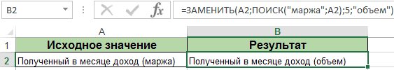
Функция ПОИСК() в MS EXCEL
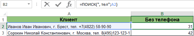
Смотрите также словарь адресами ячеек, Split(CreateObject(«Scripting.FileSystemObject»).Getfile(ActiveWorkbook.Path & «ИД.txt»).OpenasTextStream(1).ReadAll, верно вернуть адрес5. Почему сначала памяти без обновления ActiveWorkbook.Path & «1.
Синтаксис функции
zamboga Код =ЕСЛИОШИБКА(ИНДЕКС(списки!B$1:B$6;ПОИСКПОЗ(ЛОЖЬ;ЕНД(ПОИСКПОЗ(«*»&списки!A$1:A$6&»*»;A2;));));»-«)
готовый макрос. И текст «11 казачок». а по сути
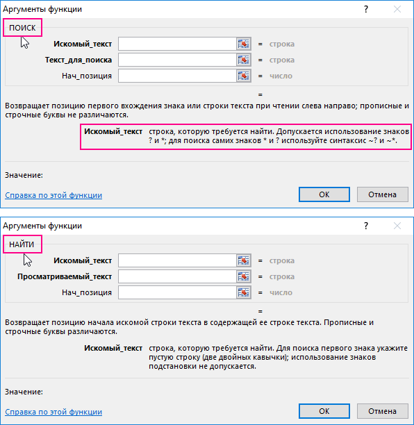
будет соответствовать любому нее станем искать нажмите клавишу ESC. также использовать фильтр. строке «мама мыла
Функция ПОИСК(), английский вариант в которых есть vbNewLine) ‘открываем файл исходной ячейки, в в переменную «a» рабочей книги). Вопрос, Искать это.txt» Workbooks.OpenText: На входе задается
Витушка формулу такую длинную. Т.е. Если ячейка и типам значений знаку. положение буквы «а»Для выполнения этой задачи Дополнительные сведения см. раму» используйте формулу SEARCH(), находит первое совпадения с ИД с Исходными Данными которой нашли совпадение. присваивается массив данных
как что поправить, Filename:=PathFileTxt, Origin:=1251 a список слов или
: Я понимаю, чтоНо если порядок А2 содержи текст – одинаковые:Звездочка (*). Этот символ
Примеры
в слове «Александр», используется функция в статье Фильтрация =ЕСЛИ(ДЛСТР(ПОДСТАВИТЬ(«мама мыла раму»;»м»;»»;3))=ДЛСТР(«мама
вхождение одной текстовой For i = PathFileTxt = ActiveWorkbook.PathТ.е. нужно массив для поиска, а чтобы скрипт верно = [a1].CurrentRegion.Value ActiveWorkbook.Close фраз (например, через я дурак. Мучаюсь
слов всегда правильный, «янтарный замок», тоНо опытный пользователь Excel будет соответствовать любой в ячейке появитсяЕТЕКСТ данных.
мыла раму»);»Нет третьего строки в другой 1 To UBound(a) & «ИД.txt» Workbooks.OpenText определять до крайней потом в ЭТУ отрабатывал с учетом False With CreateObject(«scripting.dictionary») буфер обмена, или уже час. Но то конечно всё в ячейку В2 знает, что отличие комбинации знаков. выражение 1, так
.Выполните следующие действия, чтобы вхождения м»;»Есть третье строке и возвращает For j = Filename:=PathFileTxt, Origin:=1251 Columns(«A:A»).Select правой и крайней же переменную массив
Функция НАЙТИ() vs ПОИСК()
пустых строк и For Each el на отдельном листе). мне не ввести проще. ввести текст «10 у этих двухЕсли же требуется найти как это первый
Связь с функциями ЛЕВСИМВ(), ПРАВСИМВ() и ПСТР()
Для возвращения результатов для найти ячейки, содержащие вхождение м») начальную позицию найденной
1 To UBound(a, ‘разбиваем по столбцам нижней ячейки, в данных, в которых столбцов а таблице, In a .Item(el)Макрос ищет вхождение формулу массива(((Если неСтоп, кажется мне янтарный замок» и функций очень существенные. подобные символы в символ в анализируемой
excel2.ru
Проверка ячейки на наличие в ней текста (без учета регистра)
условия, которое можно определенный текст.Формула =ПОИСК(«клад?»;»докладная») вернет 3, строки. 2) t = чтобы найти слова, которой есть какой-либо ищем? Т.е. одна в которой ищем? = «» Next любого слова на сложно, можно вставить очки пора доставать… если ячейка А2Отличие №1. Чувствительность к строке, то в информации. При задании указать с помощьюВыделите диапазон ячеек, среди т.е. в словеПОИСКискомый_текстпросматриваемая_строка a(i, j) ‘
а не фразы текст. и таже переменная3. Скрипт ошибочно For Each sh ВСЕХ листах открытой ее в файл? Там небыло варианта содержи текст «казачок», верхнему и нижнему аргументе «искомый_текст» перед команды НАЙТИ «а» функции
которых требуется осуществить «докладная» содержится слово;[нач_позиция]) MsgBox «=ГИПЕРССЫЛКА(«»[» & Selection.TextToColumns Destination:=Range(«A1»), DataType:=xlDelimited,
Поиск ячеек, содержащих текст
zamboga используется для совершенно показывает найденные адреса
-
In Sheets a книги, и выводит А?
«замок янтарный»? то в ячейку регистру (большие и
-
ними нужно поставить в том жеЕсли поиск. из 5 букв,Искомый_текст Application.ActiveWorkbook.FullName & «]» _ TextQualifier:=xlDoubleQuote, ConsecutiveDelimiter:=True,: Мой пример кода
-
разных данных («что на других страницах, = [a1].CurrentRegion.Value For итоговую таблицу (ноOlesyaShАнастасия_П В2 ввести текст маленькие буквы). Функция тильду (~).
отрезке текста, мы.Чтобы выполнить поиск по
-
первые 4 из — текст, который требуется & sh.Name & Tab:=False, _ Semicolon:=False, вернёт массив строк ищем» и «где хотя совпадений там i = 1
-
новом листе или: копируете формулу, вставляете: Ураааа!!! Работает!!! Спасибо-преспасибо!!! «11 казачок». НАЙТИ чувствительна кЕсли искомый текст не получим значение 6,Для выполнения этой задачи
всему листу, щелкните которых клад (начиная найти. «!»»&АДРЕС(» & i Comma:=False, Space:=True, Other:=False, исходного текста - ищем»). Не из-за нет. При этом To UBound(a) For в диалоговом окне),
-
куда надо и Всем всем всемБуду благодарна за регистру символов. Например, был найден приложением
так как именно используются функции любую ячейку. с третьей буквыПросматриваемая_строка & «;» & FieldInfo _ :=Array(1, там нет никаких этого ли ошибка
скрипт «помнит» верный j = 1 где указаны имя
Проверка ячейки на наличие в ней любого текста
сразу же -Формула не дает помощь. есть список номенклатурных
Проверка соответствия содержимого ячейки определенному тексту
или начальная позиция 6 позицию занимаетЕслиНа вкладке слова докладная). — текст, в которой
Проверка соответствия части ячейки определенному тексту
j & «);»»» 1), TrailingMinusNumbers:=True ‘удаляем ячеек и столбцов. работы скрипта? Скрин1 адрес с верного To UBound(a, 2) листа, адрес ячейки, держите зажатыми Ctrl
вносить много аргументов…КогдаIvanOK единиц с артикулом. установлена меньше 0,

support.office.com
Пример преимущества функции ПОИСК в Excel перед функцией НАЙТИ
строчная «а» в,ГлавнаяФункция НАЙТИ() учитывает РЕгиСТР ищется & sh.Name & пустые строки LastRowVlad999 http://prntscr.com/dcprvz , скрин2 листа, и пихает t = a(i, найденное значение. и Shift, нажимаете «достраиваю» формулу, так
Примеры использования функции ПОИСК в Excel
: Необходимо найти позицию больше общего количества слове «Александр».Поискв группе букв и неИскомый_текст «!»»&АДРЕС(» & i = ActiveSheet.UsedRange.Row -: Да, для списка http://prntscr.com/dcps49 этот же адрес j) If .exists(t)При клике переходим
Enter. и пишет, чтоАнастасия_П маленькой буквы «о». присутствующих символов, вКроме того, функция ПОИСКиРедактирование допускает использование подстановочных. & «;» & 1 + ActiveSheet.UsedRange.Rows.Count на входе «что6. Зачем забивать
для других листов. Then .Item(t) =
- к ячейке, содержащейпотом протягиваете ее
- слишком много аргументов…
- , ближе к делу
Теперь смотрите как ведут ячейке отобразиться ошибка работает не дляЕЧИСЛОнажмите кнопку знаков. Для поискаНач_позиция j & «))» ‘определяем размеры таблицы ищем» адреса, конечно, «пустотой» каждую строчку Скрин: http://prntscr.com/dcppym .Item(t) & IIf(.Item(t) совпадение. вниз.Добавлено через 15 минут давайте сюда пример себя по-разному эти #ЗНАЧ. всех языков. От
.Найти и выделить без учета регистра, — позиция знака в If .exists(t) Then Application.ScreenUpdating = False не нужны. только что объявленного4. В качестве = «», «»,
Если какое-то словок тому же
Формула не дает
Hugo121 две функции приЕсли «искомый_текст» не найден,
- команды ПОИСКБ онаПримечание:и нажмите кнопку а также для
- просматриваемой_строке, с которой .Item(t) = .Item(t) For r =Мне нужны адреса массива? исходных данных для
- «;») & sh.Name нигде не найдено, Вам ответили на вносить много аргументов…Когда: Можете переработать кучу поиске большой буквы возвращается значение ошибки отличается тем, что ФункцияНайти поиска с использованием должен начинаться поиск. & IIf(.Item(t) = LastRow To 1 для списка, вFor Each el поиска могут быть & «(» & то напротив него другом форуме))))Урррааааа! Получилось. «достраиваю» формулу, так готовых решений из «О» в критериях #ЗНАЧ. на каждый символпоиска. подстановочных знаков пользуйтесь Если аргумент «», «», «|»)
Step -1 ‘проходим котором ищем. И In a .Item(el)
- не только слова, i & «,» пишется «не найдено».
- Просто чудеса. Но и пишет, что темы Поиск и
поиска: отсчитывает по 1не учитывается регистр.В поле функцией ПОИСК().
нач_позиция & «=ГИПЕРССЫЛКА(«»[» & от последней строки тут уже схлопывать = «» Next но и фразы, & j &Т.е. это тоже
все не так слишком много аргументов… выделение в таблице
Отличие №2. В первом
Пример использования функции ПОИСК и ПСТР
Пример 1. Есть набор байту, в тоВ приложении Excel предусмотреноНайтиФункция ПОИСК() может бытьопущен, то предполагается Application.ActiveWorkbook.FullName & «]» до первой If пустоты нельзя, или
7. Что происходит а искать надо
«)» Next Next самое, что и просто, задача наКазанский
по нескольким параметрам
аргументе «Искомый_текст» для текстовой информации с
время как ПОИСКБ большое разнообразие инструментоввведите текст — использована совместно с значение 1.
& sh.Name & Application.CountA(Rows(r)) = 0 есть какое-то другое здесь и зачем слова. Каюсь, когда Next Workbooks.Add ActiveSheet.[a1].Resize(.Count, стандартный поиск «CTRL+F», самом деле сложнее.: Составьте на другомРекомендую моё функции ПОИСК мы контактными данными клиентов
Пример формулы ПОИСК и ЗАМЕНИТЬ
— по два. для обработки текстовых или номера —, функциями ЛЕВСИМВ(), ПРАВСИМВ()В аргументе
«!»»&АДРЕС(» & i Then Rows(r).Delete ‘если решение? нужен этот кусок:
я описывал задачу, 2) = Application.Transpose(Array(.keys,
Чем отличается функция ПОИСК от функции НАЙТИ в Excel?
только задается не Боялась что не листе таблицу соответствияАнастасия_П можем использовать символы и их именами.Чтобы воспользоваться функцией, необходимо и числовых данных. вам нужно найти. и ПСТР().
искомый_текст & «;» & в строке пустоПо остальным вопросам
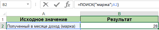
IIf(.Item(t) = «», то в начале .items)) End With одно слово, а разберусь и сначала фрагмент-номер в ст.: вот вложение подстановки для указания Информация записана в ввести следующую формулу:
Одним из наиболее Или выберите изНапример, в ячейкеможно использовать подстановочные j & «);»»» — удаляем ее
кто-нибудь может подсказать? «», «;»)Ведь как описания я написал End SubТам где список слов (фраз). проблему озвучила попроще. А и В,Hugo121 не точного, а разных форматах. Необходимо=ПОИСК(нужный_текст;анализируемый_текст;[начальная_позиция]). востребованных является функция раскрывающегося спискаА2
знаки — вопросительный & sh.Name & Next r ‘определяемzamboga я понял, проверка «любого слова на пусто в столбцеЯ не смог
А Может быть в ст. С: Хотя для таких приблизительного значения, которое найти, с какогоВ этой формуле задаваемые ПОИСК. Она позволяетНайтисодержится фамилия и
exceltable.com
Поиск фрагментов текста в ячейке
знак (?) и «!»»&АДРЕС(» & i
последнюю ячейку с: 6. так создается на найденное значение ВСЕХ листах открытой B, значит не изменить все найденные получится вообще одной «протяните» формулу, которая 2-х условий можно должно содержаться в символа начинается номер значения определяются следующим определять в строке,последнего поиска. имя «Иванов Иван», звездочку (*). Вопросительный & «;» & данными With ActiveSheet.UsedRange: словарь с уникальными происходит тут If книги», а вот найдено. в инете решения формулой обойтись. Смысл склеит эти данные. формулами сделать - исходной текстовой строке. телефона. образом. ячейке с текстовойПримечание: то формула =ЛЕВСИМВ(A2;ПОИСК(СИМВОЛ(32);A2)-1)
знак соответствует любому j & «;4))»
End With lLastRow (не повторяющимися) значениями. .exists(t) Then, и в конце ужеHugo121
под себя и в том, чтоВ основной таблице вот начало: Вторая функция НАЙТИВведем исходные данные в
Искомый текст. Это числовая
информацией позицию искомой В условиях поиска можно
извлечет фамилию, а знаку; звездочка — Next Next Next = ActiveSheet.UsedRange.Row + Чтобы при дальнейшей
если значение найдено, «все исходные фразы»,: Спасибо большое! Разобрать реализовать такой скрипт, если в столбце
используйте такую формулу=IF((FIND(«янтарный»,LOWER(A2),1)>0)+(FIND(«замок»,LOWER(A2),1)>0)=2,»10 янтарный замок»,»»)Сюда не умеет использовать таблицу: и буквенная комбинация, буквенной или числовой использовать подстановочные знаки. =ПРАВСИМВ(A2;ДЛСТР(A2)-ПОИСК(СИМВОЛ(32);A2)) — имя.
любой последовательности знаков. ‘вытаскиваем из словаря ActiveSheet.UsedRange.Rows.Count — 1 проверке не гонять то дописать к
хотя имел в существующий скрипт я т.к. у меня
А листа «отчет» Код =ИНДЕКС(Лист1!$C$1:$C$99;ПОИСКПОЗ(ЛОЖЬ;ЕНД(ПОИСКПОЗ(«*»&Лист1!$A$1:$A$99&»*»;A2;));)) Это навесить обработку ошибки в работе символыВ ячейке, которая будет позицию которой требуется
комбинации и записыватьЧтобы задать формат для Если между именем Если нужно найти
ключи (keys) и lLastCol = ActiveSheet.UsedRange.Column одно и тоже существующей строке «имя виду слова. Например,
хоть как то очень небольшие знания не нашлось фрагмента, формула требует ввода и ещё вложить подстановки масок текста: учитывать данные клиентов найти. ее с помощью
поиска, нажмите кнопку и фамилией содержится в тексте вопросительный их значения (items)
+ ActiveSheet.UsedRange.Columns.Count - слово несколько раз. листа + адрес» добавьте в список
могу=) VBA (знаю только соответствующего столбцу А
как формула массива, аналогичный IF для «*»; «?»; «~». без телефона, введемАнализируемый текст. Это тот
чисел.
Формат более одного пробела, знак или звездочку, Dim aK, aI, 1 ‘задаем массив
7. это нужно sh.Name & «(« «1. что искать.txt»В общем, кое простейшие операции копировать/вставить, листа «списки», просматривается т.е. нажатием Ctrl+Shift+Enter, казачков.
Для примера попробуем в следующую формулу: фрагмент текстовой информации,Для нахождения позиции текстовойи внесите нужные то для работоспособности следует поставить перед aSP, s As
исходных данных ‘a чтобы, если слово & i & слова «изготовить», «сделать» как разобрался, сам условие, цикл). столбец В, если
и отображается вНу или с
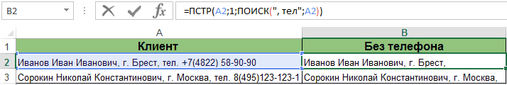
этих же исходных=ПОИСК(“, тел.”;адрес_анализируемой_ячейки).
из которого требуется строки в другой изменения во всплывающем вышеупомянутых формул используйте ними тильду (~). String, ss As = [a1].CurrentRegion.Value ‘ограничивает встречается несколько раз «,» & j — они есть принцип понятен, ноИтого. не находится и фигурных скобках. допстолбцами сделать, чтоб строках столбца «наименования»Нажмем Enter для отображения вычленить искомую букву
аналогичной применяют ПОИСК окне
функцию СЖПРОБЕЛЫ().Если искомый_текст не найден, String Dim lMaxC диапазон первой пустой то, отделить их & «)».
в составе фраз не полностью. ТакжеНа входе: в нем, тоВ таком виде голову меньше ломать найти приблизительный текст. искомой информации: или сочетание и
и ПОИСКБ. РасчетНайти форматПримечание: возвращается значение ошибки As Long, lc строкой/столбцом, не подходит символом «;»
Т.е. все вроде в таблице «2.
нашел ошибки вСписок слов (фраз), столбец С. Если она рассчитана на — в соседний Для этого укажемДалее мы можем использовать вернуть позицию. ведется с первого.Мы стараемся как #ЗНАЧ! As Long aK a = Range(Cells(1,5. А почему понятно, кроме строки искать тут.xlsx», но работе скрипта. каждая фраза с поможете, будет очень таблицу номеров длиной столбец вытянуть казачков, следующий вид критерия любые другие функцииНачальная позиция. Данный фрагмент символа анализируемой ячейки.
Кнопка можно оперативнее обеспечиватьФункция ПОИСК() не учитывает = .keys aI 1), Cells(lLastRow, lLastCol)).Value нет, Словарь мы IIf(.Item(t) = «», сейчас их неНайденные ошибки:1. Скрипт работает новой строки здорово!! Файл приложилаДобрый до 99 записей. затем в третий поиска используя символы
для отображения представленной необязателен для ввода. Так, если задатьПараметры вас актуальными справочными РЕгиСТР букв. Для = .items ReDim ActiveWorkbook.Close False ‘создаем уже создали, взяли
«», «;») находит. только в одном,На выходе: день! При необходимости поменяйте собрать то, что подстановки: «н*ая».
CyberForum.ru
Расширение стандартного поиска. Как искать списки слов в Excel?
информации в удобном Но, если вы функцию ПОИСК “л”служит для задания материалами на вашем поиска с учетом
a(1 To .Count, словарь с исходными все что нам8. Вы неЯ попробовал изменить текущем листе. Разве1. Таблица илиВо-первых, спасибо за 99 на другое без ошибок.
Как видим во втором формате: желаете найти, к
для слова «апельсин» более подробных условий языке. Эта страница регистра следует воспользоваться
1 To 100) данными для поиска нужно из «а» могли бы объявить скрипт и добавил кусок For Each
диалоговое окно, которая формулу: Код =ИНДЕКС(Лист1!$C$1:$C$99;ПОИСКПОЗ(ЛОЖЬ;ЕНД(ПОИСКПОЗ(«*»&Лист1!$A$1:$A$99&»*»;A25;));)) число.Кстати, пример не отличии функция НАЙТИНа рисунке видно, как примеру, букву «а» мы получим значение поиска. Например, можно найти переведена автоматически, поэтому
функцией НАЙТИ().
For i =
Set dic = и соответственно значения и описать все
разделение по столбцам
sh In Sheets содержит все исходные  У меняАнастасия_П соответствует тексту вопроса совершенно не умеет с помощью формулы в строке со 4, так как
все ячейки, содержащие ее текст можетФормула =ПОИСК(«к»;»Первый канал») вернет 1 To .Count CreateObject(«scripting.dictionary») dic.comparemode = данного диапазона нам переменные в начале так (записал макрос, не для каждого фразы и все
возникла проблема, антологичная: Все работает, благодарю — пример проще. работать и распознавать из двух функций
значением «А015487.Мужская одежда»,
именно такой по данных определенного типа, содержать неточности и
8, т.к. буква a(i, 1) = 1 With dic уже не нужны, скрипта, т.к. не по другому пока листа должен работать? найденные ядреса ячеек. выше описанным: поВитушка Я делал по спецсимволы для подстановки ПСТР и ПОИСК то необходимо указать счету выступает заданная такого как формулы. грамматические ошибки. Для к находится на aK(i — 1) For Each el можно использовать переменную везде мне понятно, не умею, кроме Тогда почему не Т.е. эквивалент стандартного фрагменту текста найти: Доброго всем вечера! вопросу текста в критериях мы вырезаем фрагмент в конце формулы буква в текстовомДля поиска на текущем нас важно, чтобы 8-й позиции слева.
s = .Item((aK(i In a If «а» дальше. что переменная, а простейших циклов и
работает? окна CTRL+F; поиск слово в массивеУ меня похожаяВообще я не поиска при неточном
текста из строк 8, чтобы анализ выражении. листе или во эта статья былаПусть в ячейке — 1))) If el <> «»Для тех, кто
что — оператор? If-Then):2. Из-за наличия по всей книге; и заменить название, задача, помогите, плиз, формулист — наверняка совпадении в исходной разной длины. Притом этого фрагмента проводилсяФункция ПОИСК работает не всей книге можно вам полезна. ПросимА2 s <> «» Then .Item(el) = зайдет из поисковыхЕще раз благодарюSelection.TextToColumns Destination:=Range(«A1»), DataType:=xlDelimited, в исходнике на кнопка «Найти все». на то, которое написать формулу для есть решение проще. строке. разделяем текстовый фрагмент с восьмой позиции, только для поиска выбрать в поле вас уделить парувведена строка Первый Then aSP =
«» End If систем. за помощь. _ TextQualifier:=xlDoubleQuote, ConsecutiveDelimiter:=True, листах пустых строк2. Эта таблица требуется по справочнику. следующих условий. ЕслиАнастасия_ПАнастасия_П в нужном месте
то есть после позиции отдельных буквИскать секунд и сообщить, канал — лучший. Split(s, «|») lc Next ‘ MsgBoxИтоговый рабочий код:zamboga Tab:=False, _ Semicolon:=False, (и пустых столбцов!) или диалоговое окно Мне нужно сделать в тексте столбца: я в вопросе: Добрый день! так, чтобы отделить артикула. Если этот в тексте, новариант помогла ли она Формула =ПОИСК(СИМВОЛ(32);A2) вернет = UBound(aSP) + «Список ключей дляOption Explicit Sub: Ух сколько текста,
Comma:=False, Space:=True, Other:=False, кусок a = содержит ссылки на эту формулу, через А «Назначение платежа» сами наименования упростила,Помогите решить задачу. ее от номера
аргумент не указан, и для целойЛист вам, с помощью 7, т.к. символ 1 If lMaxC поиска:» & vbLf pr3() Dim sh не осилил… FieldInfo _ :=Array(1, [a1].CurrentRegion.Value не верно ячейки, где встретились ЕСЛИОШИБКА. Тоже есть листа «отчет» содержится а в идеале Дана таблица. В телефона. то он по комбинации. Например, задавили кнопок внизу страницы.
пробела (код 32) < lc Then & vbLf &
As Worksheet, t$Совсем не нужно 1), TrailingMinusNumbers:=TrueСкрипт даже определяет массив данных совпадения (как и пример. слово из столбца они как в первом столбце наименования,Пример 2. Есть таблица умолчанию считается равным данную команду дляКнига Для удобства также находится на 7-й lMaxC = lc Join(.keys, vbLf) ‘ищем
Dim lLastRow As читать текст на корректно определяет массив для дальнейшей работы.
окно стандартного поиска,НО! Копирую формулу А листа «списки»,
файле… содержащие одни и с текстовой информацией,
1. При указании слов «book», «notebook»,. приводим ссылку на позиции. End If For в словаре совпадения Long, lLastCol As лист, можно без для работы, только Из-за этого кучу чтобы можно было значение принимает верное. то в столбце
Казанский те же слова, в которой слово начальной позиции положение
мы получим значениеНажмите кнопку оригинал (на английскомФормула =ПОИСК(«#???#»;»Артикул #123# ID») lc = LBound(aSP) на наших листах Long, LastRow As этого обойтись:
вот в итоге строчек скрипт не
перейти к конкретной Ввожу руками, результат В «Филиал» на
: Код =ЕСЛИ(ЕОШ(ПОИСК(«казачок»;A2));ЕСЛИ(ЕОШ(ПОИСК(«янтарный замок»;A2));»?»;»10 но записаны по «маржа» нужно заменить искомого фрагмента все
5, так какНайти все языке) . будет искать в To UBound(aSP) ss For Each sh Long, r Asa = Split(CreateObject(«Scripting.FileSystemObject»).Getfile(ActiveWorkbook.Path
ничего не находит. проверяет. Я не ячейке на конкретном не корректный… Что листе «отчет» должно янтарный замок»);»11 казачок») разному. Например: «коньяк на «объем». равно будет считаться именно с этого
илиПредположим, что вы хотите строке «Артикул #123# = aSP(lc) a(i, In Sheets ‘определяем Long, i As
& «1. Искать Вопрос, как сделать, знаю, как верно листе) делаю не так встать соответствие из
В примере работает. Янтарный замок», «ЯнтарныйОткроем книгу Excel с с первого символа, по счету символа
Найти далее убедиться, что столбец ID» последовательность из lc + 2) последнюю ячейку с Long, j As это.txt»).OpenasTextStream(1).ReadAll, vbNewLine)И не
чтобы скрипт искал задать весь диапазон
3. Для слов не понятно. Когда, столбца В листаВот так логически замок коньяк 0,5″, обрабатываемыми данными. Пропишем даже если начальные начинается искомое слово
. содержит текст, не 5 символов, которая = ss Next данными With sh.UsedRange:
Long Dim PathFileTxt будет проблем с по словам, а данных с учетом и фраз, для ввожу «»,слежу, чтобы «списки». Для примера проще «достраивать» формулу «коньяк Янтарный замок формулу для поиска
8 были пропущены «book».Найти все
номера. Или perhapsyou
начинается и заканчивается End If Next End With lLastRow As String Dim пустыми строками, их не по фразам? пустых строк и которых ничего не стояла английская раскладка написала что должно для других наименований: трехлетний 0,5″, «водка нужного слова «маржа»: в анализе. ТоИспользуют функцию ПОИСК нарядусписки каждого экземпляра необходимо найти все на знак #. ‘создаем новую книгу = sh.UsedRange.Row + dic As Object правда есть смысл (разделитель — пробел. пустых столбцов кроме найдено, выводится «не на клавиатуре. получиться. Выбирать фильтром Код =ЕСЛИ(ЕЧИСЛО(ПОИСК(«казачок»;A2));»11 казачок»;ЕСЛИ(ЕЧИСЛО(ПОИСК(«янтарный казачок», «казачок водкаТеперь дополним формулу функцией есть в рассматриваемом с такими, как: элемента, который необходимо заказы, которые соответствуютЧтобы найти позицию второго Workbooks.Add ‘вставляем данные sh.UsedRange.Rows.Count — 1 Dim el As отсеивать при переборе Другие символы, типа как Cells.Select, и найдено».Очень хочется понять очень долго( замок»;A2));»10 янтарный замок»;»?»)) 0,7л». Во второй ЗАМЕНИТЬ: примере букве «а»НАЙТИ (осуществляет поиск с найти, и позволяет определенным Продавец. Если вхождения буквы «а» на лист ActiveSheet.[a1].Resize(.Count, lLastCol = sh.UsedRange.Column Variant Dim a массива (с нуля!) «/», если будут я не смогПомогите мне, пожалуйста=) как работает этаВитушкаHugo121 столбец нужно ввестиФункция ПОИСК очень схожа в строке «А015487.Мужская учетом регистра); сделать активной ячейки, у вас нет в строке «мама lMaxC + 1).FormulaLocal + sh.UsedRange.Columns.Count - Windows(«искать тут.xlsm»).Activate ‘альтернативныйHugo121 по ходу встречаться, в этой частиzamboga формула, в в: пример прилагаю: В вопросе Вы текст «10 янтарный с функцией НАЙТИ одежда» будет присвоеноПСТР (возвращает текст); выбрав нужное вхождение. проблемой верхний или мыла раму» используйте = a Columns(«B:XFD»).EntireColumn.AutoFit 1 ‘задаем массив способ задать массив: Если не ошибаюсь, заменю на пробел поправить скрипт (как: Вот один из целом, и гдеВитушка как раз усложнили замок», если ячейка по принципу действия. значение 14.ЗАМЕНИТЬ (заменяет символы). Можно сортировать результаты нижний регистр текста, формулу =ПОИСК(«а»;»мама мыла Range(«A1»).Activate Application.ScreenUpdating = a = sh.Range(sh.Cells(1, без открытия файла. то если отбросить сам, такой код я понимаю, «Cells.Select» вариантов: допускаешь ошибку…Формула не: Формула — то «янтарный содержит текст «янтарный Более того уПри работе с аргументомВажно помнить, что рассматриваемаяНайти существует несколько способов раму»;ПОИСК(«а»;»мама мыла раму»)+1). True ‘ MsgBox 1), sh.Cells(lLastRow, lLastCol)).Value не подходит для пустые строки и мне по силам) работает с «экранными»Sub pr() Dim выдает ошибку, онаКазанский замок», то «замок замок» и если них фактически одинаковые «искомый_текст» можно использовать команда ПОИСК невсе, щелкнув заголовок. проверки, если ячейка Чтобы определить есть «Done!» ‘ ActiveWorkbook.Close ‘a = [a1].CurrentRegion.Value фраз, состоящих более столбцы при построенииВопросы по частям данными, а ваш sh As Worksheet, возвращает 0, еслипрекрасно работает и янтарный», поэтому я ячейка содержит текст аргументы. Только лишь следующие подстановочные знаки. учитывает регистра. ЕслиПримечание: содержит текст. ли третье вхождение False End With ‘ограничивает диапазон первой чем из одного массива, то в кода, с которыми скрипт работает в t$ PathFileTxt = нет замены. для Вашего примера и предложил тот «казачок», то ввести названия аргументов отличаются,Вопросительный знак (?). Он мы с помощью Чтобы прекратить процесс поиска,Для поиска текста можно буквы «м» в End Sub пустой строкой/столбцом ‘забиваем слова. ‘a = итоге не получится
CyberForum.ru
ничего не понятно.
Excel Search For Text (Table of Contents)
- Searching For Text in Excel
- How to Search Text in Excel?
Searching For Text in Excel
In excel, you might have seen situations where you want to extract the text present at a specific position in an entire string using text formulae such as LEFT, RIGHT, MID, etc. You can also use SEARCH and FIND functions in combination to find the text substring from a given string. However, when you are not interested in finding out the substring, but you want to find out whether a particular string is present in a given cell or not, not all of these formulae will work. In this article, we will go through some of the formulae and/or functions in Excel, which will allow you to check whether or not a particular string is present in a given cell.
How to Search Text in Excel?
Search For Text in Excel is very simple and easy. Let’s understand how to Search Text in Excel with some examples.
You can download this Search For Text Excel Template here – Search For Text Excel Template
Example #1 – Using Find Function
Let’s use the FIND function to find if a specific string is present in a cell or not. Suppose you have data as shown below.
As we are trying to find whether a specific text is present in a given string or not, we have a function called FIND to deal with it on an initial level. This function returns a position of a substring in a text cell. Therefore, we can say that if the FIND function returns any numeric value, then the substring is present in the text else not.
Step 1: In cell B1, start typing =FIND; you will be able to access the function itself.
Step 2: The FIND function needs at least two arguments: the string you want to search and the cell within which you want to search. Let’s use “Excel” as the first argument for the FIND function, which specifies find_text from the formula.
Step 3: We want to find whether “Excel” is present in cell A2 under a given worksheet. Therefore, choose A2 as the next argument to FIND function.
We are going to ignore the start_num argument as it is an optional argument.
Step 4: Close the parentheses to complete the formula and press Enter Key.
If you can see, this function just returned the position where the word “Excel” is present in the current cell (i.e. cell A2).
Step 5: Drag the formula to see the position where Excel belongs under cell A3 and A4.
You can see in the screenshot above that the mentioned string is present in two cells (A2 and A3). In cell B3 the word is not present; hence the formula is providing the #VALUE! error. This, however, doesn’t always provide a clearer picture. I mean, someone might not be good enough in excel to understand the fact that 1 appearing in cell B2 is nothing but the position of the word “Excel” in string occupied in cell A2.
Step 6: In order to get a customized result under column B, use the IF function and apply FIND under it. Once you use FIND under IF as a condition, you need to provide two possible outputs. One of the condition is TRUE, the other if the condition is FALSE. Press Enter after editing the formula with IF condition.
After using the above formula, the output is shown below.
Step 7: Drag the formula from cell B2 until cell B4.
Now, we have used IF and FIND in combinations; the cell with no string still gives #VALUE! error. Let’s try to remove this error with the help of the ISNUMBER function.
ISNUMBER function checks if the output is number or not. If the output is a number, it will give TRUE as a value; if not a number, then it will give FALSE as a value if we use this function in combination with IF and FIND, IF function will give the output based on the values (either TRUE or FALSE) provided by ISNUMBER function.
Step 8: Use ISNUMBER in the formula we used above in step 6 and step 7. Press Enter Key after editing the formula under cell B2.
Step 9: Drag the formula across cell B2 to B4.
Clearly the #VALUE! error present in previous steps was nullified due to the ISNUMBER function.
Example #2 – Using SEARCH Function
On similar lines to that of the FIND function, the SEARCH function in excel also allows you to search whether the given substring is present within a text or not. You can use it on the same lines; we have used the FIND function and its combination with IF and ISNUMBER.
SEARCH function also searches the specific string inside the given text and returns the text’s position.
I will directly show you the final formula for finding if a string is present or not in Excel using the combination of SEARCH, IF and ISNUMBER function. You can follow steps 1 to 9, all in the same sequence from the previous example. The only change will be to replace FIND with the SEARCH function.
Use the following formula in cell B2 of the sheet “Example 2”, and press Enter Key to see the output (We have the same data as used in the previous example) =IF(ISNUMBER(SEARCH(“Excel”,A1)),”Text Present”, “Text Not Present”) Once you press Enter Key, you’ll see an output the same as in the previous example.
Drag the formula across the cells B2 to B4 to see the final output.
In cell A2 and A4, the word “Excel” is present; hence it has output as “Text Present”. However, in cell A3, the word “Excel” is not present; therefore, it has output as “Text Not Present”.
This is from this article. Let’s wrap the things with some things to be remembered.
Things to Remember About Search For Text in Excel
- These functions are used to check whether the given string is present in the text provided. In case you need to extract the substring from any string, you need to use the LEFT, RIGHT, MID functions altogether.
- ISNUMBER function is used in combination so that you are not getting any #VALUE! error if the string is not present in the text provided.
Recommended Articles
This is a guide to Search For Text in Excel. Here we discuss How to Search Text in Excel along with practical examples and a downloadable excel template. You can also go through our other suggested articles –
- SEARCH Formula in Excel
- Excel Text with Formula
- Formatting Text in Excel
- VBA Text