
I have inherited a spreadsheet which contains several data tables. I know this because when I recalculate the spreadsheet takes time to recalculate the tables, and shows this in the recalculation notifier. Is there a systematic way to locate these data tables, similarly to locating links ( the spreadsheet has > 50 worksheets, so just searching sheet by sheet would be a little tedious).
asked Jul 5, 2011 at 21:34
![]()
You haven’t said / tagged what version of Excel you are using, but since you call them Tables, not Lists, I assume it is 2007 or 2010.
If you go to Formulas tab of the Ribbon > Name Manager you will see Table names listed amongst other defined names.
They show a different icon next to them, but to make things even clearer you can use the Filter button at the top right to show tables only.
As you work out what they do it is with renaming tables to sensible names (from the Table Tools > Design ribbon or the Name Manager) and possibly adding comments about their purpose to remind you later (do this in Name Manager > Edit)
answered Jul 6, 2011 at 15:32
![]()
AdamVAdamV
6,0281 gold badge22 silver badges38 bronze badges
In later versions of Excel you can:
Home -> Find & Select -> Go To
This will bring up a list of named items, including tables, that you can then navigate directly to
answered Jun 16, 2016 at 1:01
![]()
If the Name Manager shows no tables and a ctrl+F search for «=table» yields no results, but you are still calculating data tables, check for hidden tabs in your workbook that may include data tables.
That was the source of my problem.
answered Oct 30, 2015 at 22:01
![]()
1
Summary
This step-by-step article describes how to find data in a table (or range of cells) by using various built-in functions in Microsoft Excel. You can use different formulas to get the same result.
Create the Sample Worksheet
This article uses a sample worksheet to illustrate Excel built-in functions. Consider the example of referencing a name from column A and returning the age of that person from column C. To create this worksheet, enter the following data into a blank Excel worksheet.
You will type the value that you want to find into cell E2. You can type the formula in any blank cell in the same worksheet.
|
A |
B |
C |
D |
E |
||
|
1 |
Name |
Dept |
Age |
Find Value |
||
|
2 |
Henry |
501 |
28 |
Mary |
||
|
3 |
Stan |
201 |
19 |
|||
|
4 |
Mary |
101 |
22 |
|||
|
5 |
Larry |
301 |
29 |
Term Definitions
This article uses the following terms to describe the Excel built-in functions:
|
Term |
Definition |
Example |
|
Table Array |
The whole lookup table |
A2:C5 |
|
Lookup_Value |
The value to be found in the first column of Table_Array. |
E2 |
|
Lookup_Array |
The range of cells that contains possible lookup values. |
A2:A5 |
|
Col_Index_Num |
The column number in Table_Array the matching value should be returned for. |
3 (third column in Table_Array) |
|
Result_Array |
A range that contains only one row or column. It must be the same size as Lookup_Array or Lookup_Vector. |
C2:C5 |
|
Range_Lookup |
A logical value (TRUE or FALSE). If TRUE or omitted, an approximate match is returned. If FALSE, it will look for an exact match. |
FALSE |
|
Top_cell |
This is the reference from which you want to base the offset. Top_Cell must refer to a cell or range of adjacent cells. Otherwise, OFFSET returns the #VALUE! error value. |
|
|
Offset_Col |
This is the number of columns, to the left or right, that you want the upper-left cell of the result to refer to. For example, «5» as the Offset_Col argument specifies that the upper-left cell in the reference is five columns to the right of reference. Offset_Col can be positive (which means to the right of the starting reference) or negative (which means to the left of the starting reference). |
Functions
LOOKUP()
The LOOKUP function finds a value in a single row or column and matches it with a value in the same position in a different row or column.
The following is an example of LOOKUP formula syntax:
=LOOKUP(Lookup_Value,Lookup_Vector,Result_Vector)
The following formula finds Mary’s age in the sample worksheet:
=LOOKUP(E2,A2:A5,C2:C5)
The formula uses the value «Mary» in cell E2 and finds «Mary» in the lookup vector (column A). The formula then matches the value in the same row in the result vector (column C). Because «Mary» is in row 4, LOOKUP returns the value from row 4 in column C (22).
NOTE: The LOOKUP function requires that the table be sorted.
For more information about the LOOKUP function, click the following article number to view the article in the Microsoft Knowledge Base:
How to use the LOOKUP function in Excel
VLOOKUP()
The VLOOKUP or Vertical Lookup function is used when data is listed in columns. This function searches for a value in the left-most column and matches it with data in a specified column in the same row. You can use VLOOKUP to find data in a sorted or unsorted table. The following example uses a table with unsorted data.
The following is an example of VLOOKUP formula syntax:
=VLOOKUP(Lookup_Value,Table_Array,Col_Index_Num,Range_Lookup)
The following formula finds Mary’s age in the sample worksheet:
=VLOOKUP(E2,A2:C5,3,FALSE)
The formula uses the value «Mary» in cell E2 and finds «Mary» in the left-most column (column A). The formula then matches the value in the same row in Column_Index. This example uses «3» as the Column_Index (column C). Because «Mary» is in row 4, VLOOKUP returns the value from row 4 in column C (22).
For more information about the VLOOKUP function, click the following article number to view the article in the Microsoft Knowledge Base:
How to Use VLOOKUP or HLOOKUP to find an exact match
INDEX() and MATCH()
You can use the INDEX and MATCH functions together to get the same results as using LOOKUP or VLOOKUP.
The following is an example of the syntax that combines INDEX and MATCH to produce the same results as LOOKUP and VLOOKUP in the previous examples:
=INDEX(Table_Array,MATCH(Lookup_Value,Lookup_Array,0),Col_Index_Num)
The following formula finds Mary’s age in the sample worksheet:
=INDEX(A2:C5,MATCH(E2,A2:A5,0),3)
The formula uses the value «Mary» in cell E2 and finds «Mary» in column A. It then matches the value in the same row in column C. Because «Mary» is in row 4, the formula returns the value from row 4 in column C (22).
NOTE: If none of the cells in Lookup_Array match Lookup_Value («Mary»), this formula will return #N/A.
For more information about the INDEX function, click the following article number to view the article in the Microsoft Knowledge Base:
How to use the INDEX function to find data in a table
OFFSET() and MATCH()
You can use the OFFSET and MATCH functions together to produce the same results as the functions in the previous example.
The following is an example of syntax that combines OFFSET and MATCH to produce the same results as LOOKUP and VLOOKUP:
=OFFSET(top_cell,MATCH(Lookup_Value,Lookup_Array,0),Offset_Col)
This formula finds Mary’s age in the sample worksheet:
=OFFSET(A1,MATCH(E2,A2:A5,0),2)
The formula uses the value «Mary» in cell E2 and finds «Mary» in column A. The formula then matches the value in the same row but two columns to the right (column C). Because «Mary» is in column A, the formula returns the value in row 4 in column C (22).
For more information about the OFFSET function, click the following article number to view the article in the Microsoft Knowledge Base:
How to use the OFFSET function
Need more help?
Want more options?
Explore subscription benefits, browse training courses, learn how to secure your device, and more.
Communities help you ask and answer questions, give feedback, and hear from experts with rich knowledge.
Содержание
- Lookup Table in Excel
- How to Create a Lookup Table in Excel?
- #1 – Create a Lookup Table Using VLOOKUP Function
- #2 – Use LOOKUP Function to Create a LOOKUP Table in Excel
- #3 – Use INDEX + MATCH Function
- Things to Remember
- Recommended Articles
- Look up values with VLOOKUP, INDEX, or MATCH
- Using INDEX and MATCH instead of VLOOKUP
- Give it a try
- VLOOKUP Example at work
- Find a table in excel and understand formula
- 2 Answers 2
- Use Excel built-in functions to find data in a table or a range of cells
- Summary
- Create the Sample Worksheet
- Term Definitions
- Functions
- LOOKUP()
- VLOOKUP()
- INDEX() and MATCH()
- OFFSET() and MATCH()
Lookup Table in Excel


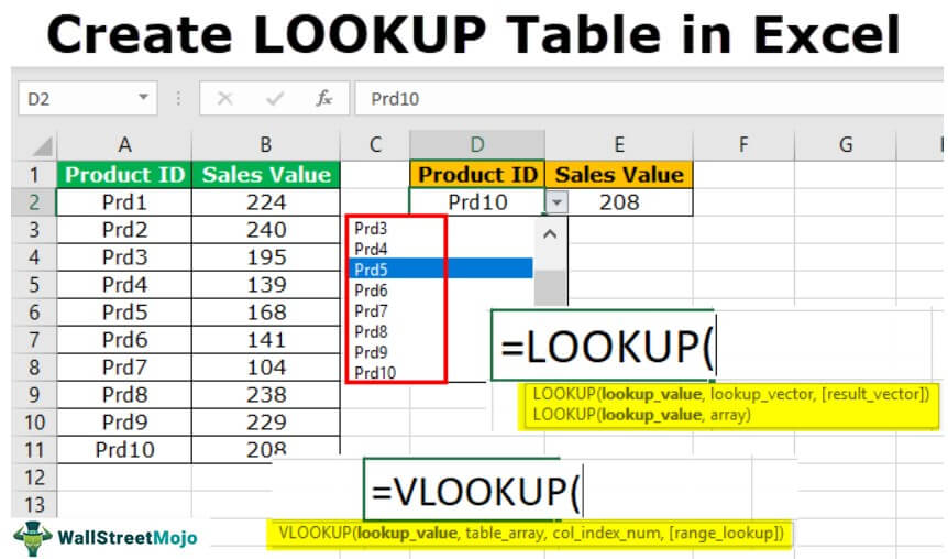
LOOKUP tables in Excel are named tables used with the VLOOKUP function to find any data. When we have a large amount of data and do not know where to look, we can select the table and name it. While using the VLOOKUP function, instead of providing the reference, we can type the table’s name as a reference to look up the value. Such a table is known as a lookup table in Excel.
How to Create a Lookup Table in Excel?
LOOKUP functions are lifesavers in Excel. Based on the available or lookup value, we can fetch the other data in different tables. In Excel, VLOOKUP is the most commonly used LOOKUP function.
This article will discuss some of the important lookup functions in Excel and how to create a lookup table in Excel. Important lookup functions are VLOOKUP and HLOOKUP, V stands for vertical lookup, and H stands for horizontal lookup. We have the function called LOOKUP to look for the data in the table.
You are free to use this image on your website, templates, etc., Please provide us with an attribution link How to Provide Attribution? Article Link to be Hyperlinked
For eg:
Source: Lookup Table in Excel (wallstreetmojo.com)
We can fetch the available data and other information from different worksheets and workbooks using these LOOKUP functions.
Table of contents
#1 – Create a Lookup Table Using VLOOKUP Function
- Lookup Value is nothing but the available value. Based on this value, we are trying to fetch the data from the other table.
- Table Array is simply the main table where all the information resides.
- Col Index Num is nothing but from which column of the table array we want the data. So we need to mention the column number here.
- Range Lookup is nothing but whether you are looking for an exact match or an approximate match. If you are looking for the same match, then FALSE or 0 is the argument. If you are looking for the approximate match, then TRUE or 1 is the argument.
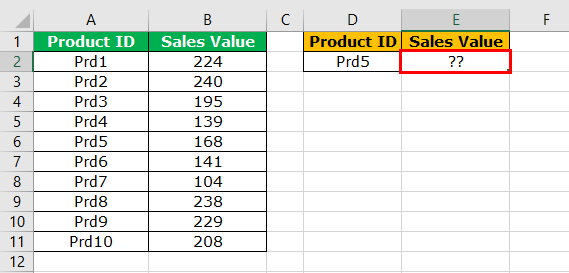
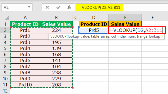
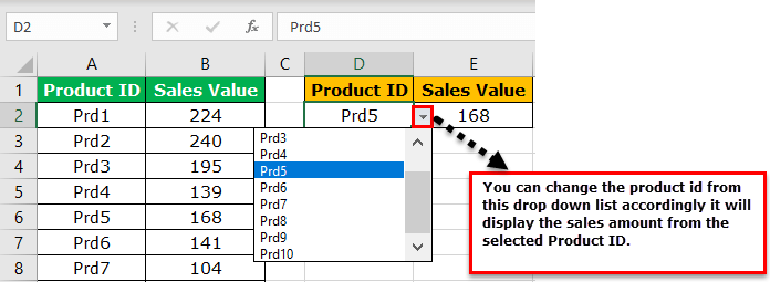
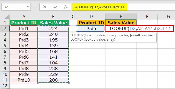
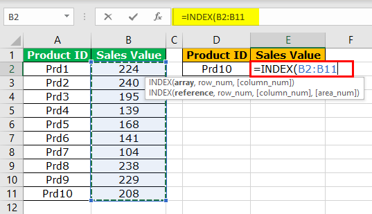
Example of VLOOKUP Function: Assume below is the data you have of product sales and their sales amount.

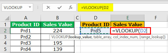
Now, in cell D2, we have one product ID, and using this product ID, we have to fetch the sales value using VLOOKUP.
Follow these steps:
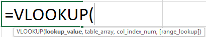
- We must apply the VLOOKUP function and open the formula first.
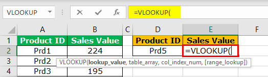
The first argument is the LOOKUP value. It is our base or available value. So, we must select cell D2 as the reference.
Next is the table array. It is nothing but our main table where all the data resides. So, select the table array as A2 to B11.
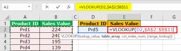
Now, press the F4 function key to make it an absolute excel reference. It will insert the dollar symbol into the selected cell.
The next argument is the column index number from the selected table from which column we are looking for the data. In this case, we have chosen two columns, and we need the data from the second column, so we must mention 2 as the argument.
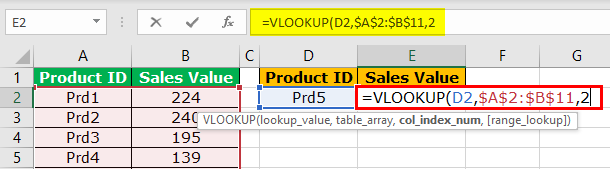
The final argument is range lookup, i.e., type of lookup. Since we are looking at an exact match, we must select FALSE or insert zero as the argument.
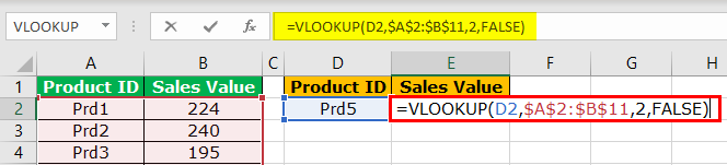
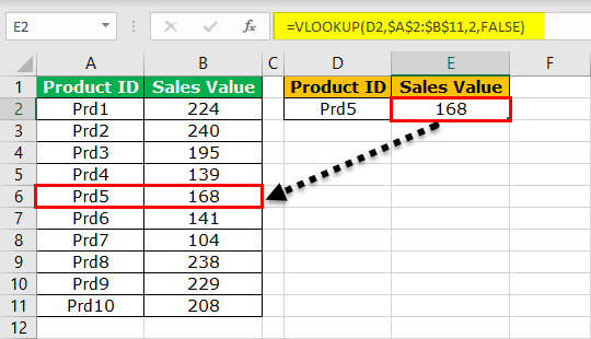
Close the bracket and press the “Enter” key. We should have the sales value for the product ID Prd5.
What if we want the sales data for the product if Prd6. Of course, we can enter directly, but this is not the right approach. Rather, we can create the drop-down list in excel and allow the user to select from the drop-down list. Press ALT + A + V + V in cell D2. It is the shortcut key, which is the shortcut key to create data validation in excel.
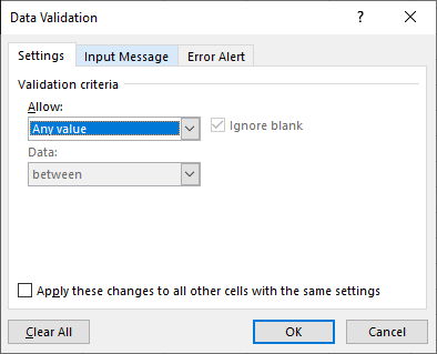
Select the “LIST” from the “Allow:” drop-down.
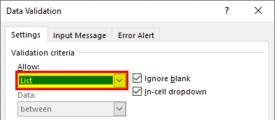
In the “SOURCE:” select the Product ID list from A2 to A11.
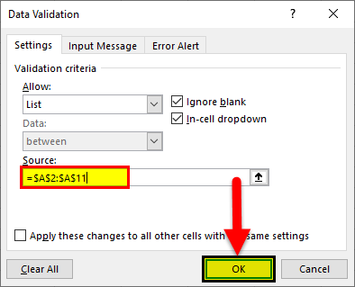
Click on the “OK.” We have all the list of products in cell D2 now.
#2 – Use LOOKUP Function to Create a LOOKUP Table in Excel
Let’s apply the formula to understand the logic of the LOOKUP function.
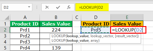
Step 1: We must open the LOOKUP function now.

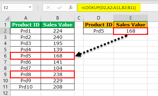
Step 2: The lookup value is product ID, so select the D2 cell.
Step 3: The lookup vector is nothing but the product ID column in the main table. So select A1 to A11 as the range.
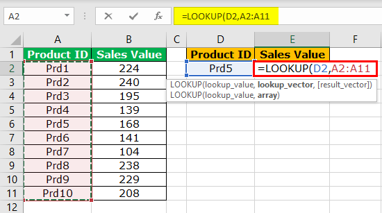
Step 4: Next is the results vector. It is nothing but from which column we need the data to be fetched. In this case, from B1 to B11, we want the data to be brought.
Step 5: Close the bracket and press the “Enter” key to close the formula. We should have sales value for the selected product ID.
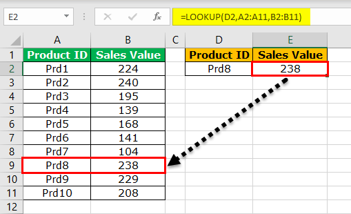
Step 6: Change the product ID to see a different result.
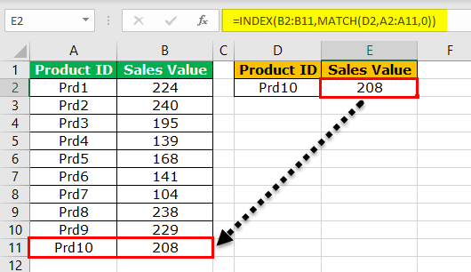
#3 – Use INDEX + MATCH Function
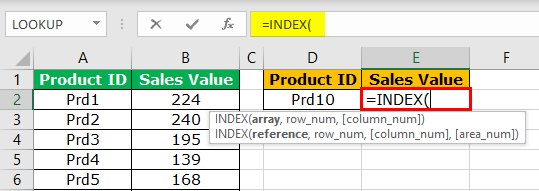
Step 2: Select the result column in the main table for the first argument.
Step 3: To get the row number, we need to apply the MATCH function. Refer to the below image for the MATCH function.
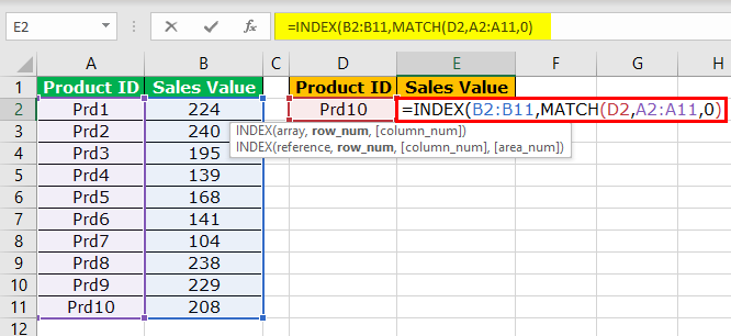
Step 4: Close the bracket and close the formula. We will have results.
Things to Remember
- The LOOKUP should be the same as in the main table in Excel.
- The VLOOKUP function works from left to right, not from right to left.
- In the LOOKUP function, we need to select the result column and need not mention the column index number, unlike VLOOKUP.
Recommended Articles
This article is a guide to the LOOKUP Table in Excel. We discuss creating a LOOKUP table in Excel using VLOOKUP, INDEX, MATCH formulas, practical examples, and a downloadable Excel template. You may also learn more about Excel from the following articles: –
Источник
Look up values with VLOOKUP, INDEX, or MATCH
Tip: Try using the new XLOOKUP and XMATCH functions, improved versions of the functions described in this article. These new functions work in any direction and return exact matches by default, making them easier and more convenient to use than their predecessors.
Suppose that you have a list of office location numbers, and you need to know which employees are in each office. The spreadsheet is huge, so you might think it is challenging task. It’s actually quite easy to do with a lookup function.
The VLOOKUP and HLOOKUP functions, together with INDEX and MATCH, are some of the most useful functions in Excel.
Note: The Lookup Wizard feature is no longer available in Excel.
Here’s an example of how to use VLOOKUP.
In this example, B2 is the first argument—an element of data that the function needs to work. For VLOOKUP, this first argument is the value that you want to find. This argument can be a cell reference, or a fixed value such as «smith» or 21,000. The second argument is the range of cells, C2-:E7, in which to search for the value you want to find. The third argument is the column in that range of cells that contains the value that you seek.
The fourth argument is optional. Enter either TRUE or FALSE. If you enter TRUE, or leave the argument blank, the function returns an approximate match of the value you specify in the first argument. If you enter FALSE, the function will match the value provide by the first argument. In other words, leaving the fourth argument blank—or entering TRUE—gives you more flexibility.
This example shows you how the function works. When you enter a value in cell B2 (the first argument), VLOOKUP searches the cells in the range C2:E7 (2nd argument) and returns the closest approximate match from the third column in the range, column E (3rd argument).
The fourth argument is empty, so the function returns an approximate match. If it didn’t, you’d have to enter one of the values in columns C or D to get a result at all.
When you’re comfortable with VLOOKUP, the HLOOKUP function is equally easy to use. You enter the same arguments, but it searches in rows instead of columns.
Using INDEX and MATCH instead of VLOOKUP
There are certain limitations with using VLOOKUP—the VLOOKUP function can only look up a value from left to right. This means that the column containing the value you look up should always be located to the left of the column containing the return value. Now if your spreadsheet isn’t built this way, then do not use VLOOKUP. Use the combination of INDEX and MATCH functions instead.
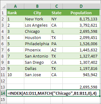
This example shows a small list where the value we want to search on, Chicago, isn’t in the leftmost column. So, we can’t use VLOOKUP. Instead, we’ll use the MATCH function to find Chicago in the range B1:B11. It’s found in row 4. Then, INDEX uses that value as the lookup argument, and finds the population for Chicago in the 4th column (column D). The formula used is shown in cell A14.
For more examples of using INDEX and MATCH instead of VLOOKUP, see the article https://www.mrexcel.com/excel-tips/excel-vlookup-index-match/ by Bill Jelen, Microsoft MVP.
Give it a try
If you want to experiment with lookup functions before you try them out with your own data, here’s some sample data.
VLOOKUP Example at work
Copy the following data into a blank spreadsheet.
Tip: Before you paste the data into Excel, set the column widths for columns A through C to 250 pixels, and click Wrap Text ( Home tab, Alignment group).
Источник
Find a table in excel and understand formula
I have inherited a spreadsheet with an IRR calculation that has the following formula:
I would guess it is a structured reference referring to a table, but I can’t find the table.
Q1: What is the formula doing? It pulls in an NPV amount, which is then used for IRR, so it seems to be some sort of look up.
Q2: If a formula is referring to a table, how do I find the table? I can see many tables being recalculated, but can’t find them.
2 Answers 2
This is a data table, normally produced from (in Excel 2007) Data > Data Tools> What-if Analysis > Data Table.
It seems to be a 2-way table so the reference formula should be in the top-left cell of the table. E47 and C41 will be referred to in this formula, and the data table substitutes these values with the values in the leading row and column of the data table. You can use this feature to produce, for instance, a multiplication table.
See the following for more information:

I found that the easiest to way to go to the Table referred in a formula (See Example 1 below), is to use the Pull down menu, called the Name Box, just above Column A, to the left of the Formula bar (See Picture 1 below).
This is the same Pull down we use when we ‘name’ our own group of cells. Tags: Excel Table Identification. Where is my Excel Table?
Источник
Use Excel built-in functions to find data in a table or a range of cells
Summary
This step-by-step article describes how to find data in a table (or range of cells) by using various built-in functions in Microsoft Excel. You can use different formulas to get the same result.
Create the Sample Worksheet
This article uses a sample worksheet to illustrate Excel built-in functions. Consider the example of referencing a name from column A and returning the age of that person from column C. To create this worksheet, enter the following data into a blank Excel worksheet.
You will type the value that you want to find into cell E2. You can type the formula in any blank cell in the same worksheet.
Term Definitions
This article uses the following terms to describe the Excel built-in functions:
The whole lookup table
The value to be found in the first column of Table_Array.
Lookup_Array
-or-
Lookup_Vector
The range of cells that contains possible lookup values.
The column number in Table_Array the matching value should be returned for.
3 (third column in Table_Array)
Result_Array
-or-
Result_Vector
A range that contains only one row or column. It must be the same size as Lookup_Array or Lookup_Vector.
A logical value (TRUE or FALSE). If TRUE or omitted, an approximate match is returned. If FALSE, it will look for an exact match.
This is the reference from which you want to base the offset. Top_Cell must refer to a cell or range of adjacent cells. Otherwise, OFFSET returns the #VALUE! error value.
This is the number of columns, to the left or right, that you want the upper-left cell of the result to refer to. For example, «5» as the Offset_Col argument specifies that the upper-left cell in the reference is five columns to the right of reference. Offset_Col can be positive (which means to the right of the starting reference) or negative (which means to the left of the starting reference).
Functions
LOOKUP()
The LOOKUP function finds a value in a single row or column and matches it with a value in the same position in a different row or column.
The following is an example of LOOKUP formula syntax:
The following formula finds Mary’s age in the sample worksheet:
The formula uses the value «Mary» in cell E2 and finds «Mary» in the lookup vector (column A). The formula then matches the value in the same row in the result vector (column C). Because «Mary» is in row 4, LOOKUP returns the value from row 4 in column C (22).
NOTE: The LOOKUP function requires that the table be sorted.
For more information about the LOOKUP function, click the following article number to view the article in the Microsoft Knowledge Base:
VLOOKUP()
The VLOOKUP or Vertical Lookup function is used when data is listed in columns. This function searches for a value in the left-most column and matches it with data in a specified column in the same row. You can use VLOOKUP to find data in a sorted or unsorted table. The following example uses a table with unsorted data.
The following is an example of VLOOKUP formula syntax:
The following formula finds Mary’s age in the sample worksheet:
The formula uses the value «Mary» in cell E2 and finds «Mary» in the left-most column (column A). The formula then matches the value in the same row in Column_Index. This example uses «3» as the Column_Index (column C). Because «Mary» is in row 4, VLOOKUP returns the value from row 4 in column C (22).
For more information about the VLOOKUP function, click the following article number to view the article in the Microsoft Knowledge Base:
INDEX() and MATCH()
You can use the INDEX and MATCH functions together to get the same results as using LOOKUP or VLOOKUP.
The following is an example of the syntax that combines INDEX and MATCH to produce the same results as LOOKUP and VLOOKUP in the previous examples:
The following formula finds Mary’s age in the sample worksheet:
The formula uses the value «Mary» in cell E2 and finds «Mary» in column A. It then matches the value in the same row in column C. Because «Mary» is in row 4, the formula returns the value from row 4 in column C (22).
NOTE: If none of the cells in Lookup_Array match Lookup_Value («Mary»), this formula will return #N/A.
For more information about the INDEX function, click the following article number to view the article in the Microsoft Knowledge Base:
OFFSET() and MATCH()
You can use the OFFSET and MATCH functions together to produce the same results as the functions in the previous example.
The following is an example of syntax that combines OFFSET and MATCH to produce the same results as LOOKUP and VLOOKUP:
This formula finds Mary’s age in the sample worksheet:
The formula uses the value «Mary» in cell E2 and finds «Mary» in column A. The formula then matches the value in the same row but two columns to the right (column C). Because «Mary» is in column A, the formula returns the value in row 4 in column C (22).
For more information about the OFFSET function, click the following article number to view the article in the Microsoft Knowledge Base:
Источник
Содержание
- 1 Простой поиск
- 2 Расширенный поиск
- 3 Разновидности поиска
- 3.1 Поиск совпадений
- 3.2 Фильтрация
- 3.3 Видео: Поиск в таблице Excel
Рубрика Excel
Также статьи о работе с таблицами в Экселе:
- Форматирование таблиц в Excel
- Создание таблиц в excel
- Создание сводной таблицы в excel
- Как выделить всю таблицу целиком в excel?
Среди тысяч строк и десятков столбцов данных вручную в таблице Эксель найти что-то практически невозможно. Единственный вариант, это воспользоваться какой-то функцией поиска, и далее мы рассмотрим, как осуществляется поиск в таблице Excel.
Для осуществления поиска данных в таблице Excel необходимо использовать пункт меню «Найти и выделить» на вкладке «Главная», в котором нужно выбирать вариант «Найти» или воспользоваться для вызова комбинацией клавиш «Ctrl + F».
Для примера попробуем найти необходимое число среди данных нашей таблицы, так как именно при поиске чисел необходимо учитывать некоторые тонкости поиска. Будем искать в таблице Excel число «10».
После выбора необходимого пункта меню в появившемся окошке поиска вводим искомое значение. У нас два варианта поиска значений в таблице Эксель, это найти сразу все совпадения нажав кнопку «Найти все» или сразу же просматривать каждую найденную ячейку, нажимая каждый раз кнопку «Найти далее». При использовании кнопки «Найти далее» следует также учитывать текущее расположение активной ячейки, так как поиск начнется именно с этой позиции.

Попробуем найти сразу все значения, при этом все найденное будет перечислено в окошке под настройкой поиска. Если оставить все настройки по умолчанию, то результат поиска будет не совсем такой, как мы ожидали.

Для правильного поиска данных в таблице Эксель следует нажать кнопку «Параметры» и произвести настройку области поиска. Сейчас же искомое значение ищется даже в формулах, используемых в ячейках для расчетов. Нам же необходимо указать поиск только в значениях и при желании можно еще указать формат искомых данных.

При поиске слов в таблице Excel следует также учитывать все эти тонкости и к примеру, можно учитывать даже регистр букв.
Ну и на последок рассмотрим, как сделать поиск данных в Экселе только в необходимой области листа. Как видно из нашего примера, искомое значение «10» встречается сразу во всех столбцах данных. Если необходимо это значение найти, допустим, только в первом столбце, необходимо выделить данный столбец или любую область значений, в которой необходимо произвести поиск, а затем уже приступать к поиску.

В нашем первом столбце имеется только два значения, равных «10», поэтому при применении варианта «Найти все» в списке должно появиться только два результата поиска.

Таблицы в Excel представляют собой ряд строк и столбцов со связанными данными, которыми вы управляете независимо друг от друга.
Работая в Excel с таблицами, вы сможете создавать отчеты, делать расчеты, строить графики и диаграммы, сортировать и фильтровать информацию.
Если ваша работа связана с обработкой данных, то навыки работы с таблицами в Эксель помогут вам сильно сэкономить время и повысить эффективность.
Как работать в Excel с таблицами. Пошаговая инструкция
Прежде чем работать с таблицами в Эксель, последуйте рекомендациям по организации данных:
- Данные должны быть организованы в строках и столбцах, причем каждая строка должна содержать информацию об одной записи, например о заказе;
- Первая строка таблицы должна содержать короткие, уникальные заголовки;
- Каждый столбец должен содержать один тип данных, таких как числа, валюта или текст;
- Каждая строка должна содержать данные для одной записи, например, заказа. Если применимо, укажите уникальный идентификатор для каждой строки, например номер заказа;
- В таблице не должно быть пустых строк и абсолютно пустых столбцов.
1. Выделите область ячеек для создания таблицы

Выделите область ячеек, на месте которых вы хотите создать таблицу. Ячейки могут быть как пустыми, так и с информацией.
2. Нажмите кнопку “Таблица” на панели быстрого доступа
На вкладке “Вставка” нажмите кнопку “Таблица”.
3. Выберите диапазон ячеек

В всплывающем вы можете скорректировать расположение данных, а также настроить отображение заголовков. Когда все готово, нажмите “ОК”.
4. Таблица готова. Заполняйте данными!

Поздравляю, ваша таблица готова к заполнению! Об основных возможностях в работе с умными таблицами вы узнаете ниже.
Форматирование таблицы в Excel
Для настройки формата таблицы в Экселе доступны предварительно настроенные стили. Все они находятся на вкладке “Конструктор” в разделе “Стили таблиц”:
Если 7-ми стилей вам мало для выбора, тогда, нажав на кнопку, в правом нижнем углу стилей таблиц, раскроются все доступные стили. В дополнении к предустановленным системой стилям, вы можете настроить свой формат.
Помимо цветовой гаммы, в меню “Конструктора” таблиц можно настроить:
- Отображение строки заголовков – включает и отключает заголовки в таблице;
- Строку итогов – включает и отключает строку с суммой значений в колонках;
- Чередующиеся строки – подсвечивает цветом чередующиеся строки;
- Первый столбец – выделяет “жирным” текст в первом столбце с данными;
- Последний столбец – выделяет “жирным” текст в последнем столбце;
- Чередующиеся столбцы – подсвечивает цветом чередующиеся столбцы;
- Кнопка фильтра – добавляет и убирает кнопки фильтра в заголовках столбцов.
Как добавить строку или столбец в таблице Excel
Даже внутри уже созданной таблицы вы можете добавлять строки или столбцы. Для этого кликните на любой ячейке правой клавишей мыши для вызова всплывающего окна:
- Выберите пункт “Вставить” и кликните левой клавишей мыши по “Столбцы таблицы слева” если хотите добавить столбец, или “Строки таблицы выше”, если хотите вставить строку.

- Если вы хотите удалить строку или столбец в таблице, то спуститесь по списку в сплывающем окне до пункта “Удалить” и выберите “Столбцы таблицы”, если хотите удалить столбец или “Строки таблицы”, если хотите удалить строку.

Как отсортировать таблицу в Excel
Для сортировки информации при работе с таблицей, нажмите справа от заголовка колонки “стрелочку”, после чего появится всплывающее окно:

В окне выберите по какому принципу отсортировать данные: “по возрастанию”, “по убыванию”, “по цвету”, “числовым фильтрам”.
Как отфильтровать данные в таблице Excel
Для фильтрации информации в таблице нажмите справа от заголовка колонки “стрелочку”, после чего появится всплывающее окно:

- “Текстовый фильтр” отображается когда среди данных колонки есть текстовые значения;
- “Фильтр по цвету” также как и текстовый, доступен когда в таблице есть ячейки, окрашенные в отличающийся от стандартного оформления цвета;
- “Числовой фильтр” позволяет отобрать данные по параметрам: “Равно…”, “Не равно…”, “Больше…”, “Больше или равно…”, “Меньше…”, “Меньше или равно…”, “Между…”, “Первые 10…”, “Выше среднего”, “Ниже среднего”, а также настроить собственный фильтр.
- В всплывающем окне, под “Поиском” отображаются все данные, по которым можно произвести фильтрацию, а также одним нажатием выделить все значения или выбрать только пустые ячейки.
Если вы хотите отменить все созданные настройки фильтрации, снова откройте всплывающее окно над нужной колонкой и нажмите “Удалить фильтр из столбца”. После этого таблица вернется в исходный вид.
Как посчитать сумму в таблице Excel
Для того чтобы посчитать сумму колонки в конце таблицы, нажмите правой клавишей мыши на любой ячейке и вызовите всплывающее окно:
В списке окна выберите пункт “Таблица” => “Строка итогов”:
Внизу таблица появится промежуточный итог. Нажмите левой клавишей мыши на ячейке с суммой.
В выпадающем меню выберите принцип промежуточного итога: это может быть сумма значений колонки, “среднее”, “количество”, “количество чисел”, “максимум”, “минимум” и т.д.
Как в Excel закрепить шапку таблицы
Таблицы, с которыми приходится работать, зачастую крупные и содержат в себе десятки строк. Прокручивая таблицу “вниз” сложно ориентироваться в данных, если не видно заголовков столбцов. В Эксель есть возможность закрепить шапку в таблице таким образом, что при прокрутке данных вам будут видны заголовки колонок.
Для того чтобы закрепить заголовки сделайте следующее:
- Перейдите на вкладку “Вид” в панели инструментов и выберите пункт “Закрепить области”:
- Выберите пункт “Закрепить верхнюю строку”:
- Теперь, прокручивая таблицу, вы не потеряете заголовки и сможете легко сориентироваться где какие данные находятся:
Как перевернуть таблицу в Excel
Представим, что у нас есть готовая таблица с данными продаж по менеджерам:
На таблице сверху в строках указаны фамилии продавцов, в колонках месяцы. Для того чтобы перевернуть таблицу и разместить месяцы в строках, а фамилии продавцов нужно:
- Выделить таблицу целиком (зажав левую клавишу мыши выделить все ячейки таблицы) и скопировать данные (CTRL+C):
- Переместить курсор мыши на свободную ячейку и нажать правую клавишу мыши. В открывшемся меню выбрать “Специальная вставка” и нажать на этом пункте левой клавишей мыши:
- В открывшемся окне в разделе “Вставить” выбрать “значения” и поставить галочку в пункте “транспонировать”:
- Готово! Месяцы теперь размещены по строкам, а фамилии продавцов по колонкам. Все что остается сделать – это преобразовать полученные данные в таблицу.
В этой статье вы ознакомились с принципами работы в Excel с таблицами, а также основными подходами в их создании. Пишите свои вопросы в комментарии!
Основное назначение офисной программы Excel – осуществление расчётов. Документ этой программы (Книга) может содержать много листов с длинными таблицами, заполненными числами, текстом или формулами. Автоматизированный быстрый поиск позволяет найти в них необходимые ячейки.
Простой поиск
Чтобы произвести поиск значения в таблице Excel, необходимо на вкладке «Главная» открыть выпадающий список инструмента «Найти и заменить» и щёлкнуть пункт «Найти». Тот же эффект можно получить, используя сочетание клавиш Ctrl + F.
В простейшем случае в появившемся окне «Найти и заменить» надо ввести искомое значение и щёлкнуть «Найти всё».
Как видно, в нижней части диалогового окна появились результаты поиска. Найденные значения подчёркнуты красным в таблице. Если вместо «Найти все» щёлкнуть «Найти далее», то сначала будет произведён поиск первой ячейки с этим значением, а при повторном щелчке – второй.
Аналогично производится поиск текста. В этом случае в строке поиска набирается искомый текст.
Если данные или текст ищется не во всей экселевской таблице, то область поиска предварительно должна быть выделена.
Расширенный поиск
Предположим, что требуется найти все значения в диапазоне от 3000 до 3999. В этом случае в строке поиска следует набрать 3???. Подстановочный знак «?» заменяет собой любой другой.
Анализируя результаты произведённого поиска, можно отметить, что, наряду с правильными 9 результатами, программа также выдала неожиданные, подчёркнутые красным. Они связаны с наличием в ячейке или формуле цифры 3.
Можно удовольствоваться большинством полученных результатов, игнорируя неправильные. Но функция поиска в эксель 2010 способна работать гораздо точнее. Для этого предназначен инструмент «Параметры» в диалоговом окне.
Щёлкнув «Параметры», пользователь получает возможность осуществлять расширенный поиск. Прежде всего, обратим внимание на пункт «Область поиска», в котором по умолчанию выставлено значение «Формулы».
Это означает, что поиск производился, в том числе и в тех ячейках, где находится не значение, а формула. Наличие в них цифры 3 дало три неправильных результата. Если в качестве области поиска выбрать «Значения», то будет производиться только поиск данных и неправильные результаты, связанные с ячейками формул, исчезнут.
Для того чтобы избавиться от единственного оставшегося неправильного результата на первой строчке, в окне расширенного поиска нужно выбрать пункт «Ячейка целиком». После этого результат поиска становимся точным на 100%.
Такой результат можно было бы обеспечить, сразу выбрав пункт «Ячейка целиком» (даже оставив в «Области поиска» значение «Формулы»).
Теперь обратимся к пункту «Искать».
Если вместо установленного по умолчанию «На листе» выбрать значение «В книге», то нет необходимости находиться на листе искомых ячеек. На скриншоте видно, что пользователь инициировал поиск, находясь на пустом листе 2.
Следующий пункт окна расширенного поиска – «Просматривать», имеющий два значения. По умолчанию установлено «по строкам», что означает последовательность сканирования ячеек по строкам. Выбор другого значения – «по столбцам», поменяет только направление поиска и последовательность выдачи результатов.
При поиске в документах Microsoft Excel, можно использовать и другой подстановочный знак – «*». Если рассмотренный «?» означал любой символ, то «*» заменяет собой не один, а любое количество символов. Ниже представлен скриншот поиска по слову Louisiana.
Иногда при поиске необходимо учитывать регистр символов. Если слово louisiana будет написано с маленькой буквы, то результаты поиска не изменятся. Но если в окне расширенного поиска выбрать «Учитывать регистр», то поиск окажется безуспешным. Программа станет считать слова Louisiana и louisiana разными, и, естественно, не найдёт первое из них.
Разновидности поиска
Поиск совпадений
Иногда бывает необходимо обнаружить в таблице повторяющиеся значения. Чтобы произвести поиск совпадений, сначала нужно выделить диапазон поиска. Затем, на той же вкладке «Главная» в группе «Стили», открыть инструмент «Условное форматирование». Далее последовательно выбрать пункты «Правила выделения ячеек» и «Повторяющиеся значения».
Результат представлен на скриншоте ниже.
При необходимости пользователь может поменять цвет визуального отображения совпавших ячеек.
Фильтрация
Другая разновидность поиска – фильтрация. Предположим, что пользователь хочет в столбце B найти числовые значения в диапазоне от 3000 до 4000.
- Выделить первый столбец с заголовком.
- На той же вкладке «Главная» в разделе «Редактирование» открыть инструмент «Сортировка и фильтр», и щёлкнуть пункт «Фильтр».
- В верхней строчке столбца B появляется треугольник – условный знак списка. После его открытия в списке «Числовые фильтры» щёлкнуть пункт «между».
- В окне «Пользовательский автофильтр» следует ввести начальное и конечное значение плюс OK.
Как видно, отображаться стали только строки, удовлетворяющие введённому условию. Все остальные оказались временно скрытыми. Для возврата к начальному состоянию следует повторить шаг 2.
Различные варианты поиска были рассмотрены на примере Excel 2010. Как сделать поиск в эксель других версий? Разница в переходе к фильтрации есть в версии 2003. В меню «Данные» следует последовательно выбрать команды «Фильтр», «Автофильтр», «Условие» и «Пользовательский автофильтр».
Видео: Поиск в таблице Excel
LOOKUP tables in Excel are named tables used with the VLOOKUP function to find any data. When we have a large amount of data and do not know where to look, we can select the table and name it. While using the VLOOKUP function, instead of providing the reference, we can type the table’s name as a reference to look up the value. Such a table is known as a lookup table in Excel.
How to Create a Lookup Table in Excel?
LOOKUP functions are lifesavers in Excel. Based on the available or lookup value, we can fetch the other data in different tables. In Excel, VLOOKUP is the most commonly used LOOKUP function.
This article will discuss some of the important lookup functions in Excel and how to create a lookup table in Excel. Important lookup functions are VLOOKUP and HLOOKUP, V stands for vertical lookup, and H stands for horizontal lookup. We have the function called LOOKUP to look for the data in the table.
We can fetch the available data and other information from different worksheets and workbooks using these LOOKUP functions.
Table of contents
- How to Create a Lookup Table in Excel?
- #1 – Create a Lookup Table Using VLOOKUP Function
- #2 – Use LOOKUP Function to Create a LOOKUP Table in Excel
- #3 – Use INDEX + MATCH Function
- Things to Remember
- Recommended Articles
You can download this Create LOOKUP Table Excel Template here – Create LOOKUP Table Excel Template
#1 – Create a Lookup Table Using VLOOKUP Function
As we said, VLOOKUP is the traditional lookup functionThe VLOOKUP excel function searches for a particular value and returns a corresponding match based on a unique identifier. A unique identifier is uniquely associated with all the records of the database. For instance, employee ID, student roll number, customer contact number, seller email address, etc., are unique identifiers.
read more most users use regularly. Therefore, we will show you how to look for values using this LOOKUP function.
- Lookup Value is nothing but the available value. Based on this value, we are trying to fetch the data from the other table.
- Table Array is simply the main table where all the information resides.
- Col Index Num is nothing but from which column of the table array we want the data. So we need to mention the column number here.
- Range Lookup is nothing but whether you are looking for an exact match or an approximate match. If you are looking for the same match, then FALSE or 0 is the argument. If you are looking for the approximate match, then TRUE or 1 is the argument.
Example of VLOOKUP Function: Assume below is the data you have of product sales and their sales amount.
Now, in cell D2, we have one product ID, and using this product ID, we have to fetch the sales value using VLOOKUP.
Follow these steps:
- We must apply the VLOOKUP function and open the formula first.

- The first argument is the LOOKUP value. It is our base or available value. So, we must select cell D2 as the reference.

- Next is the table array. It is nothing but our main table where all the data resides. So, select the table array as A2 to B11.

- Now, press the F4 function key to make it an absolute excel reference. It will insert the dollar symbol into the selected cell.

- The next argument is the column index number from the selected table from which column we are looking for the data. In this case, we have chosen two columns, and we need the data from the second column, so we must mention 2 as the argument.

- The final argument is range lookup, i.e., type of lookup. Since we are looking at an exact match, we must select FALSE or insert zero as the argument.

- Close the bracket and press the “Enter” key. We should have the sales value for the product ID Prd5.

- What if we want the sales data for the product if Prd6. Of course, we can enter directly, but this is not the right approach. Rather, we can create the drop-down list in excel and allow the user to select from the drop-down list. Press ALT + A + V + V in cell D2. It is the shortcut key, which is the shortcut key to create data validation in excel.

- Select the “LIST” from the “Allow:” drop-down.

- In the “SOURCE:” select the Product ID list from A2 to A11.
- Click on the “OK.” We have all the list of products in cell D2 now.

#2 – Use LOOKUP Function to Create a LOOKUP Table in Excel
Instead of VLOOKUP, we can also use the LOOKUP function in excelThe LOOKUP excel function searches a value in a range (single row or single column) and returns a corresponding match from the same position of another range (single row or single column). The corresponding match is a piece of information associated with the value being searched.
read more as an alternative. But, first, let us look at the formula of the LOOKUP function.
- Lookup Value is the base value or available value.
- Lookup Vector is nothing but a lookup value column in the main table.
- Result Vector is nothing but requires a column in the main table.
Let’s apply the formula to understand the logic of the LOOKUP function.
Step 1: We must open the LOOKUP function now.
Step 2: The lookup value is product ID, so select the D2 cell.
Step 3: The lookup vector is nothing but the product ID column in the main table. So select A1 to A11 as the range.
Step 4: Next is the results vector. It is nothing but from which column we need the data to be fetched. In this case, from B1 to B11, we want the data to be brought.
Step 5: Close the bracket and press the “Enter” key to close the formula. We should have sales value for the selected product ID.
Step 6: Change the product ID to see a different result.
#3 – Use INDEX + MATCH Function
The VLOOKUP function can fetch the data from left to the right, but with the help of the INDEX FunctionThe INDEX function in Excel helps extract the value of a cell, which is within a specified array (range) and, at the intersection of the stated row and column numbers.read more and MATCH formula in excelThe MATCH function looks for a specific value and returns its relative position in a given range of cells. The output is the first position found for the given value. Being a lookup and reference function, it works for both an exact and approximate match. For example, if the range A11:A15 consists of the numbers 2, 9, 8, 14, 32, the formula “MATCH(8,A11:A15,0)” returns 3. This is because the number 8 is at the third position.
read more, we can bring data from anywhere to create a LOOKUP Excel table.
Step 1: Open the INDEX formula ExcelThe INDEX function in Excel helps extract the value of a cell, which is within a specified array (range) and, at the intersection of the stated row and column numbers.read more first.
Step 2: Select the result column in the main table for the first argument.
Step 3: To get the row number, we need to apply the MATCH function. Refer to the below image for the MATCH function.
Step 4: Close the bracket and close the formula. We will have results.
Things to Remember
- The LOOKUP should be the same as in the main table in Excel.
- The VLOOKUP function works from left to right, not from right to left.
- In the LOOKUP function, we need to select the result column and need not mention the column index number, unlike VLOOKUP.
Recommended Articles
This article is a guide to the LOOKUP Table in Excel. We discuss creating a LOOKUP table in Excel using VLOOKUP, INDEX, MATCH formulas, practical examples, and a downloadable Excel template. You may also learn more about Excel from the following articles: –
- LOOKUP Formula ExcelThe LOOKUP excel function searches a value in a range (single row or single column) and returns a corresponding match from the same position of another range (single row or single column). The corresponding match is a piece of information associated with the value being searched.
read more - VLOOKUP from Another SheetVlookup is a function that can be used to refer to columns on the same sheet or from another worksheet or workbook. A different workbook or worksheet is used to select the table array and index number.read more
- What are the Alternatives to Vlookup?To reference data in columns from right to left, we can combine the index and match functions, which is one of the best Excel alternatives to Vlookup.read more
- How to Fix VLOOKUP Errors?The top four VLOOKUP errors are — #N/A Error, #NAME? Error, #REF! Error, #VALUE! Error.read more
Lookup Table in Excel (Table of Content)
- Lookup Table in Excel
- How to Use Lookup Table in Excel?
Lookup Table in Excel
The lookup function is not as famous to use as Vlookup and Hlookup; here, we need to understand that it always returns the approximate match when we perform the Lookup function. So there is no true or false argument as it was in Vlookup and Hlookup function. In this topic, we are going to learn about Lookup Table in Excel.
Whenever lookup finds an exact match in the lookup vector, it returns the corresponding value in a given cell, and when it doesn’t find an exact match, it goes back and returns the most recent possible value but from the previous row.
Whenever we have the larger value available in the lookup table or lookup value, it returns the last value from the table, and when we have lower than the lowest, it will return #N/A, as we have understood the same in our previous example.
Remember the below formula for Lookup:
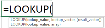
=Lookup(Lookup Value, Lookup Vector, result vector)
Here let us know the arguments:
Lookup Value: The value we are searching
Lookup Vector: Range of lookup value – (1 Row of 1 Column)
Result Vector: Must be the same size as lookup vector; it’s optional
- It can be used in many ways, i.e. Grading of students, Categorizing, retrieve approx. Position, Age group, etc.
- The lookup function assumes Lookup Vector is in ascending order.
How to Use Lookup Table in Excel?
Here we have explained how to use Lookup Table in Excel with the following examples as given below.
You can download this Lookup Table Excel Template here – Lookup Table Excel Template
Example #1
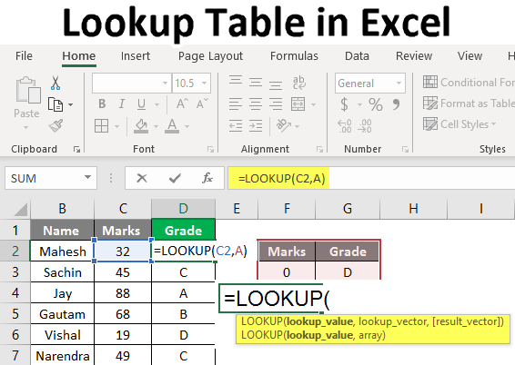
- For this example, we need data from the school students with their names and marks in a particular subject. Now, as we can see in the below image, we have the data of the students as required.
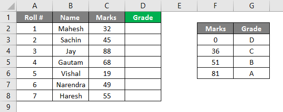
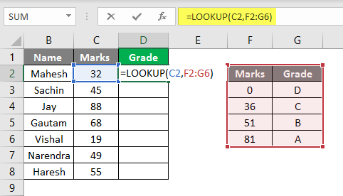
- Here also, we need a lookup vector, the value which defines marks in grades. We can see the image; at the right side of the image, we have decided the criteria for every grade; we will have to make it in ascending order because, as you all know, Look up every time assumes that the data is in ascending order. Now, as you can see, we have entered our formula in D2 Column, =lookup(C2, F2: G6). Here C2 is the lookup value, and F2: G6 is the lookup table/lookup vector.
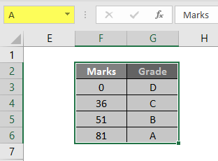
- We can define our lookup table by assigning it a name as any alphabet, let’s assume A, so we can write A instead if it’s range F2: G6. So as per the below image, you can see that we have given the name to our grade table is A.
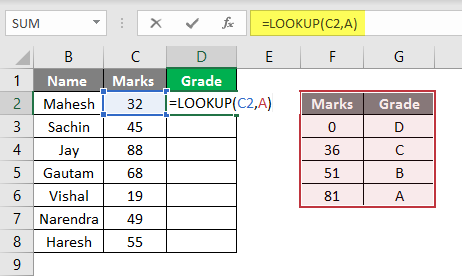
- Now while applying the formula, we can place A instead of its range, the same you can see in the below Image. We have applied the formula as =lookup(C2, A), so here C2 is our lookup value, and A is our lookup table or range of lookup.
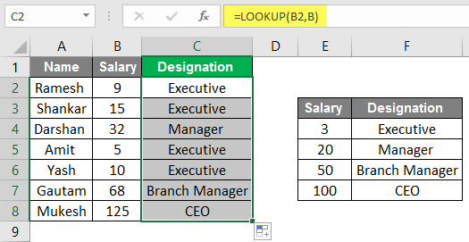
- Now we can see that as Mahesh’s marks are 32, so from our lookup/grade table, the lookup will start to look for the value 32 and till 35 marks and its grade as D, so it will show Grade ‘D.’
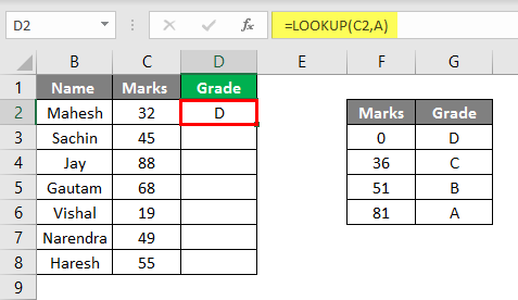
- If we drag the same till D8, we can see the grades of all the students as per the below image.
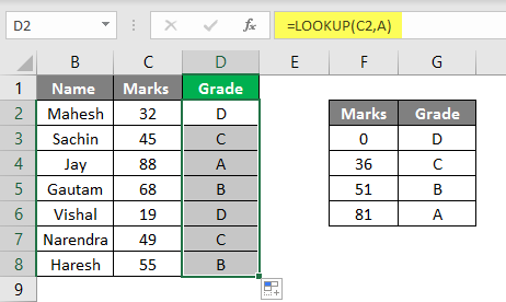
- As per the above image, you can see that we have derived the Grade from the Provided Marks. Similarly, we can use this formula for other purposes; let’s see another example.
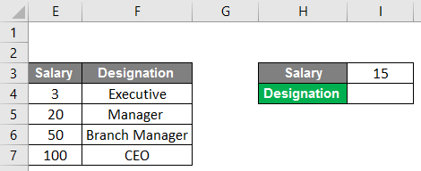
Example #2
- Like the above table, here we have gathered the data of a company with Name, their salary, and their designations. From the below image, we can see that we have given the name “B” to our lookup table.
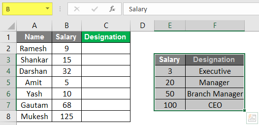
- Now we need the data to be filled in the designation column, So here we will put the formula in C2.
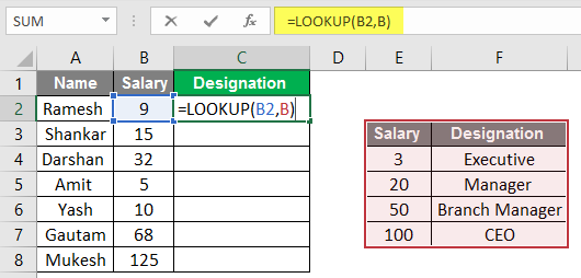
- Here we can see the Result in the Designation Column.
- Now we can see that after dragging we have fetched the designations of the staff according to their salary. We have operated this operation same as a recent example, here instead of marks we have considered the salary of employees and instead of Grade we have considered the designation.
- So we can use this formula for our different purposes academic, personal, and sometimes while making rate cards of a business model to categorize the things in manners of costly things and cheap things.
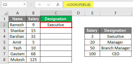
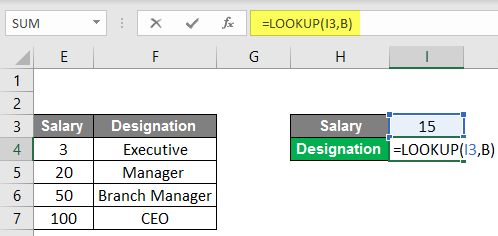
Example #3
- Here as improvisation, we can make a simulator by using a lookup formula; As per the below image, we can see we have used the same data, and instead of the table now, we can put data.
- We can see here in cell no. I4 we have applied the lookup formula, so whenever we put a value in cell no. I3, our lookup formula will look into the data and put the appropriate designation in the cell.
- For example, we have taken the value 15 as salary, so the formula will look up into the table and provide us with the designation according to the table, which is Executive.
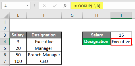
- So accordingly, we can put any value in the cell, But here is a catch, whenever we put a value that is higher than 100, it will show the designation as CEO, and when we put a value lower than 3, it will show #N/A.
Conclusion
The lookup function can lookup value from a single column or a single row of the range. Lookup value always returns a value on a vector; Lookups are of two types of lookup Vector and lookup array. Lookup can be used for various purposes; as we have seen above examples, Lookup can be used in Grading for students we can make age groups and also for the various works.
Things to Remember About Lookup Table in Excel
- While using this function, we have to remember that this function assumes that the lookup table or vector is sorted in ascending order.
- And you must know that this formula is not case sensitive.
- This formula always performs the approximate match, so true or false like arguments will not take place with the formula.
- It can only lookup to a one-column range.
Recommended Articles
This has been a guide to Lookup Table in Excel. Here we have discussed How to Use Lookup Table in Excel along with Examples and a downloadable excel template. You may also look at these useful functions in excel –
- Excel Lookup Function
- LOOKUP Formula in Excel
- VBA LOOKUP
- VLOOKUP Table Array
Searching a Microsoft Excel spreadsheet may seem easy. While Ctrl + F can help you find most things in a spreadsheet, you’ll want to use more sophisticated tools to find and extract data based on specific values. We’ll help you save tons of time with our list of advanced search functions.
Once you know how to search in Excel using lookup, it won’t matter how big your spreadsheets get, you’ll always be able to find what you need!
1. The VLOOKUP Function
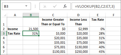
The VLOOKUP function lets you find a specific value within a column and extract values from the corresponding row in adjoining columns. Two examples where you might do this are (1) looking up an employee’s last name by their employee number, or (2) finding a phone number by specifying the last name.
Here’s the syntax of the function:
=VLOOKUP([lookup_value], [table_array], [col_index_num], [range_lookup])
- [lookup_value] is the piece of information that you already have. For example, if you need to know what state a city is in, it would be the name of the city.
- [table_array] lets you specify the cells in which the function will look for the lookup and return values. When selecting your range, be sure that the first column included in your array is the one that will include your lookup value!
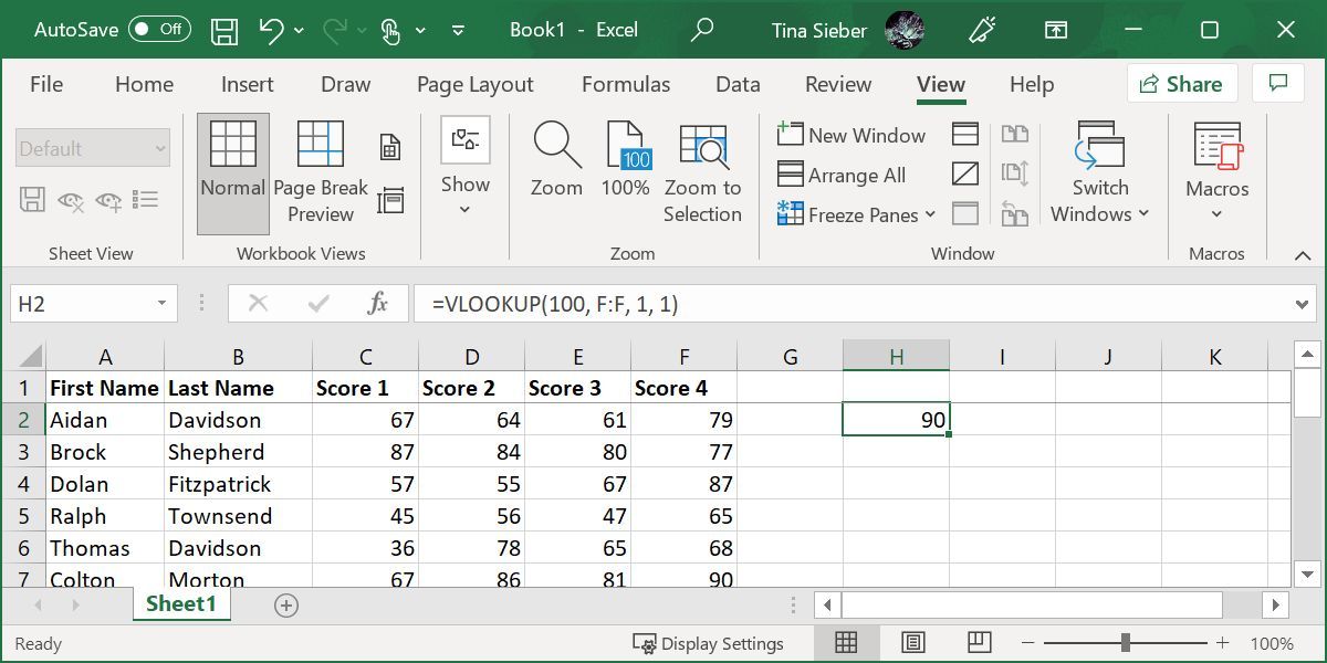
- [col_index_num] is the number of the column that contains the return value.
- [range_lookup] is an optional argument, and takes 1 or 0, though you could also enter TRUE or FALSE. If you enter 1 or omit this argument, the function looks for an approximate value, but we’ve found this to be hit-or-miss. In the example below, a VLOOKUP looking for a score of 100 returns 90. Looking for a lower value, for example 88, returned an error.
Let’s take a look at how you might use this. This spreadsheet contains student names and scores for four different tests. Let’s say you want to find score #4 for the student with the last name «Davidson.» VLOOKUP makes it easy.
Here’s the formula you’d use:
=VLOOKUP("Davidson
Because the fourth score is the fifth column over from the last name we’re looking for, 5 is the column index argument. Note that when you’re looking for text, setting [range_lookup] to 0 is a good idea. Without it, you can get bad results.
Here’s the result:
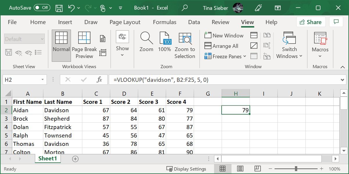
It returned 79, which is score #4 of the student we queried.
Notes on VLOOKUP
A few things are good to remember when you’re using VLOOKUP. Make sure that the first column in your range is the one that includes your lookup value. If it’s not in the first column, the function will return incorrect results. If your columns are well organized, this shouldn’t be a problem.
Also, keep in mind that VLOOKUP will only ever return one value. There was another student with the last name «Davidson,» but VLOOKUP will only ever return results for the first entry, with no indication that there is more than one match.
2. The HLOOKUP Function
Where VLOOKUP finds corresponding values in another column, HLOOKUP finds corresponding values in a different row. Because it’s usually easiest to scan through column headings until you find the right one and use a filter to find what you’re looking for, HLOOKUP is best used when you have huge spreadsheets, or if you’re working with values that are organized by time.
Here’s the syntax of the function:
=HLOOKUP([lookup_value], [table_array], [row_index_num], [range_lookup])
- [lookup_value] is the value that you know and want to find a corresponding value for.
- [table_array] is the cells in which you want to search.
- [row_index_num] specifies the row that the return value will come from.
- [range_lookup] is the same as in VLOOKUP, leave it blank to get the nearest value when possible, or enter 0 to only look for exact matches.
We’ll use the same spreadsheet as before. You can use HLOOKUP to find the score for a specific row. Here’s how we’ll do it:
=HLOOKUP("Score 4"
As you can see in the image below, the score is returned:
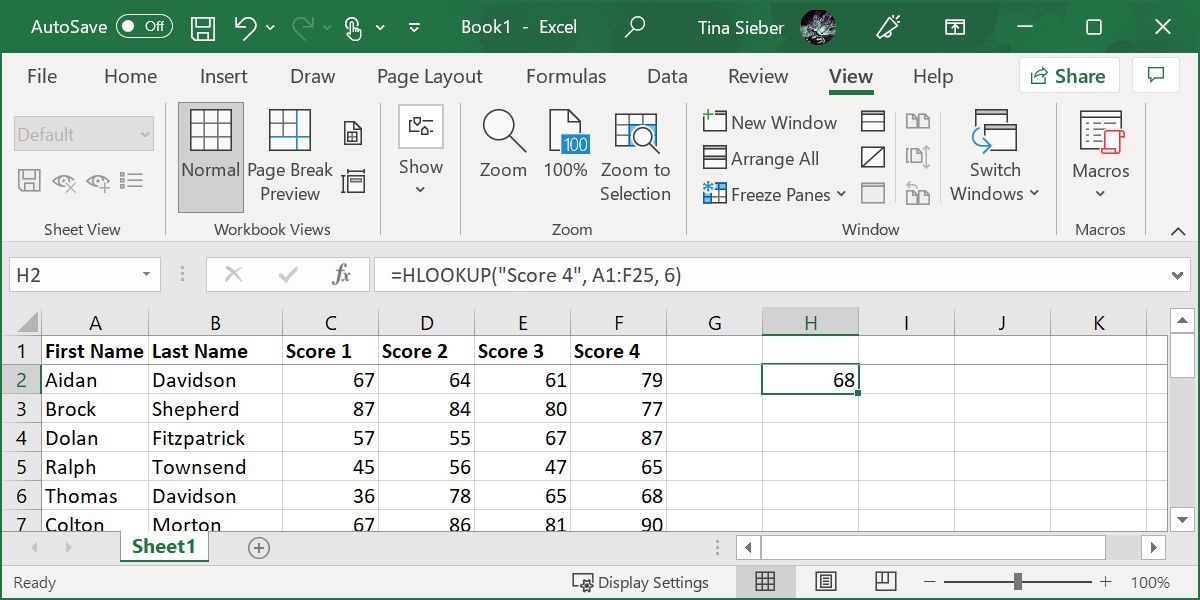
The student in row 6, Thomas Davidson, had a score of 68 on his fourth test.
Notes on HLOOKUP
As with VLOOKUP, the lookup value needs to be in the first row of your table array. This is rarely an issue with HLOOKUP, as you’ll usually be using a column title for a lookup value. HLOOKUP also only returns a single value.
3-4. The INDEX and MATCH Functions
INDEX and MATCH are two different functions, but when they’re used together, they can make searching a large spreadsheet a lot faster. Both functions have drawbacks, but by combining them, we’ll build on the strengths of both.
First, though, the syntax of both functions:
=INDEX([array], [row_number], [column_number])
- [array] is the array in which you’ll be searching.
- [row_number] and [column_number] can be used to narrow your search (we’ll take a look at that in a moment).
=MATCH([lookup_value], [lookup_array], [match_type])
- [lookup_value] is a search term that can be a string or a number.
- [lookup_array] is the array in which Microsoft Excel will look for the search term.
- [match_type] is an optional argument that can be 1, 0, or -1. 1 will return the largest value that is smaller than or equal to your search term. 0 will only return your exact term, and -1 will return the smallest value that is greater than or equal to your search term.
It might not be clear how we’re going to use these two functions together, so I’ll lay it out here. MATCH takes a search term and returns a cell reference. In the image below, you can see that in a search for the last name «Davidson» in column B, MATCH returns 2.

INDEX, on the other hand, does the opposite: it takes a cell reference and returns the value in it. You can see here that, when told to return the second row of column B, INDEX returns «Davidson,» the value from row 2.
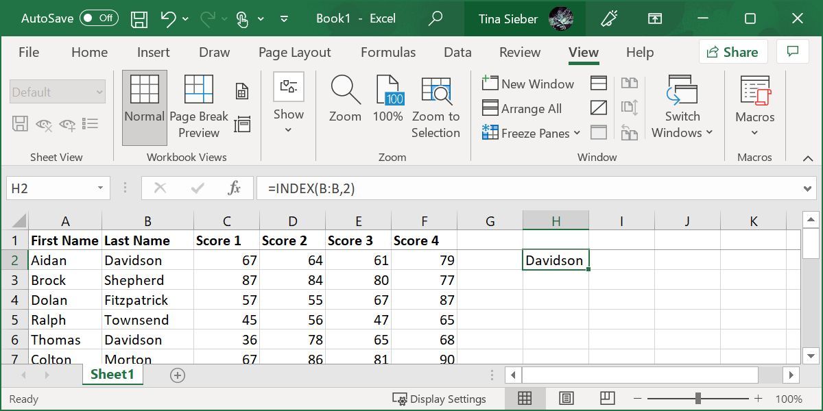
What we’re going to do is combine the two so that MATCH returns a cell reference and INDEX uses that reference to look up the value in a cell. Let’s say you remember that there was a student whose last name was Townsend, and you want to see what this student’s fourth score was. Here’s the formula we’ll use:
=INDEX(F:F, MATCH("Townsend", B:B, 0))
You’ll notice that the match type is set to 0 here. When you’re looking for a string, that’s what you’ll want to use. Here’s what we get when we run that function:
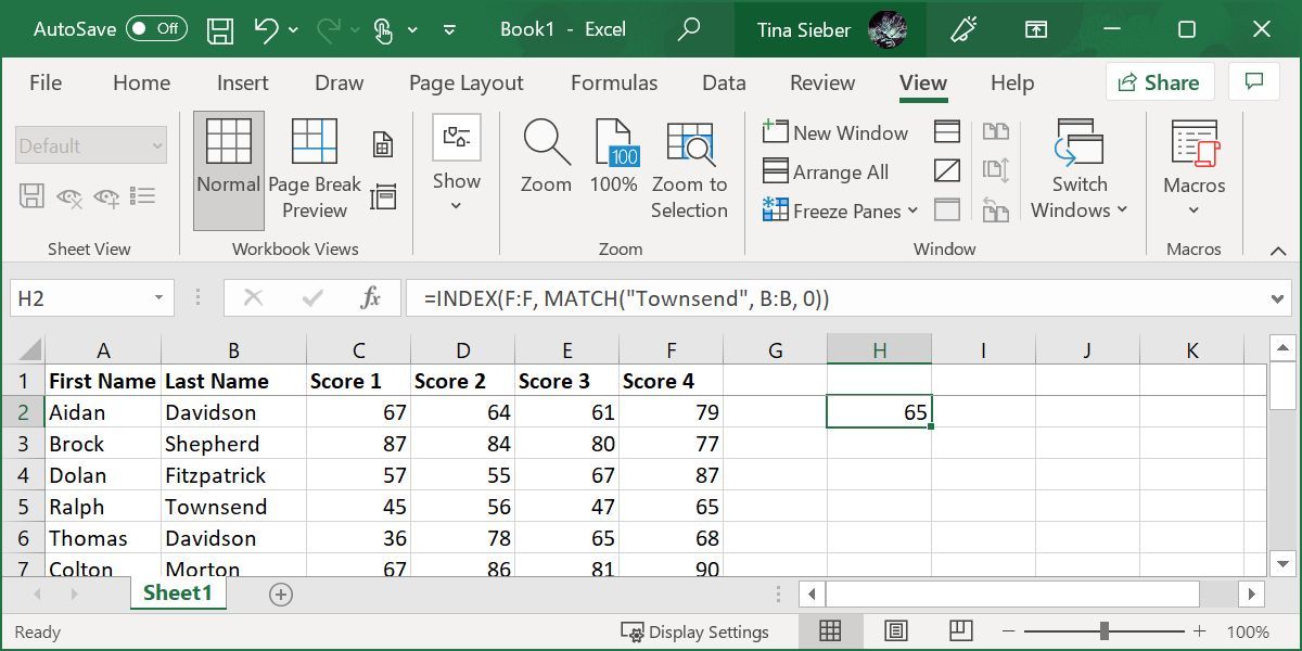
As you can see from the inset, Ralph Townsend scored a 68 in his fourth test, the number that appears when we run the function. This may not seem all that useful when you can just look a few columns over, but imagine how much time you’d save if you had to do it 50 times on a large database spreadsheet that contained several hundred columns!
5. The FIND Function
An article on finding something in Excel wouldn’t be complete without the FIND function. But it might not be what you expect. You can use Excel’s FIND function to identify the position of a string of text within another string of text.
Let’s say, we wanted to find the first occurrence of the letter «x» in the phrase «The brown fox jumped over the fence.» This would be our function:
=FIND("x", "The brown fox jumped over the fence")
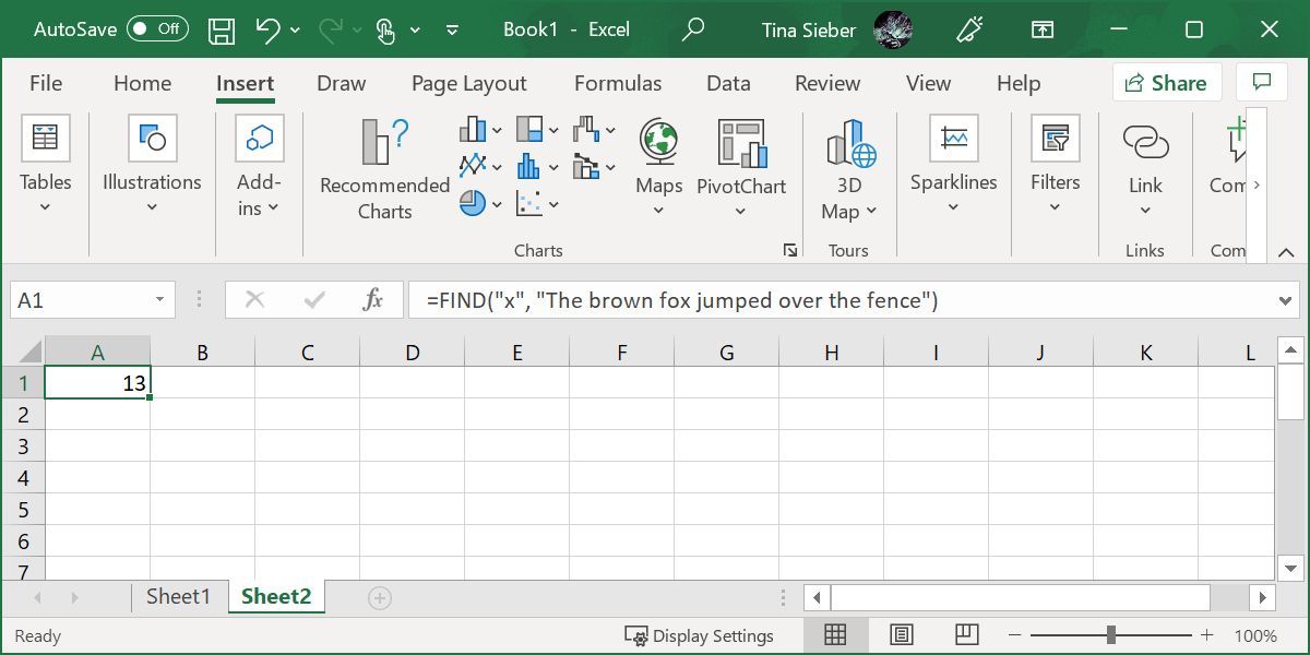
The resulting number represents the position of the queried string. If you’re looking for a multi-character string, let’s say we queried for «fox,» the result would indicate the position of the query’s first character; in this case 11.
Notes on FIND
Like VLOOKUP, HLOOKUP, and other functions, FIND will only identify the first occurrence of a string. Note that FIND is case-sensitive. You can use it to FIND multiple characters. And while we used a letter in our example, it also works with numbers.
On its own, this function might not seem very useful, but it comes into its own when you start nesting functions. For example, you could use your FIND result to split a string of text at the position corresponding to the string identified with FIND.
FIND vs. SEARCH
We can’t cover FIND without mentioning the SEARCH function. Well, it’s essentially the same as FIND, except that it’s not case-sensitive. It also allows wildcards, meaning you can search for matches that aren’t exact.
Excel supports three wildcards:
- Asterisk (*), which is a placeholder for any number of characters, including zero.
- Question mark (?), which can replace any one character.
- Tilde (~), which turns the wildcards «asterisk» and «question mark» into literal characters, meaning it cancels their wildcard function. You’d use it as ~* or ~?.
6. The XLOOKUP Function
XLOOKUP is a new function designed to replace VLOOKUP. Like VLOOKUP, you can use it to find things in a table or range by searching for a known value. It differs from VLOOKUP in that it lets you look up values located in columns to the left or right of the queried value; with VLOOKUP you can only ever find data to the right of the queried column.
Here’s the syntax of the function:
=XLOOKUP(lookup_value, lookup_array, return_array, [if_not_found], [match_mode], [search_mode])
- [lookup_value] is the value you’re searching for; i.e. your query.
- [lookup_array] is the array or range to search.
- [return_array] is the array or range to return. This is the first difference from VLOOKUP.
- [if_not_found] is an optional argument that returns a message of your choice if no match is found.
- [match_mode] is another optional argument that lets you find exact matches (0), the next smaller item (-1), the next larger item (1), or a wildcard match (2).
- [search_mode] is optional and lets you control in which order to search. The default (1) starts the search at the first item. You can also start at the last item (-1), perform a binary search that depends on the lookup_array being sorted in ascending (2) or descending (-2) order.
Let’s take our VLOOKUP example and reverse the search order. This should let us find the score of the second student called Davidson. Here’s the formula:
=XLOOKUP(G2,B2:B25,F2:F25,,,-1)
Note that we’re pulling the name from column G2, rather than writing it directly into the formula. Below is what it looks like.
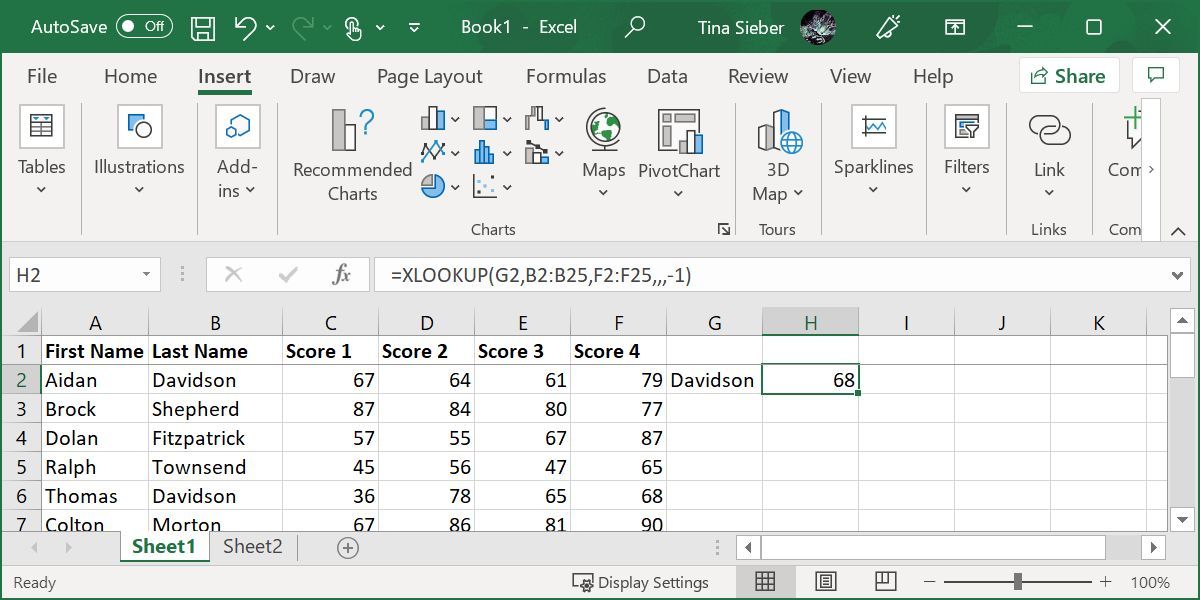
This time, the formula returned Thomas Davidson’s score, rather than that of Aidan Davidson. But it still can’t return more than one result.
Let the Excel Searches Begin
Microsoft Excel has a lot of extremely powerful functions for manipulating data, and the four listed above just scratch the surface. Learning how to use them will make your life much easier.
In this tutorial, we will take an in-depth look at some formulas you can use to query a table.
Tables are great in supporting structured referencing; hence, we can use basic formulas to carry out lots of tasks on excel. Without much ado, let’s start.

Steps for Querying a table in Excel
We will work on an excel worksheet containing a table – Table 1. The table contains the personal data of the staff of an organization. We can use many formulas to carry out various queries on these data.
1. Firstly, we will start with the ROWS Function, which we can use to count the rows on the table. It considers only the rows that contain data while counting. There are 15 types of cars on the list.
Here is the formula for the Row function:
=ROWS(Table3)

2. We also have the COLUMNS function, which counts the number of columns on the table and considers only the columns containing data.
Below is the formula:
=COLUMNS(Table3)

3. Now, if you desire to decipher the total number of cells on the table, you can combine the ROWS and the COLUMNS functions.
Look below for the combo formula.
=ROWS(Table3)*COLUMNS(Table3)

5. Simply use the COUNTBLANK function when you wish to count the cells that contain no data.
=COUNTBLANK(Table1)

6. Another important function is the SUBTOTAL function, which is used in counting visible rows. It is efficient in keeping references to columns that have no empty cells.
The value for ID is a necessity in this case. The ID column represents the reference, and I entered 103 in place of the function number.
=SUBTOTAL(103,Table1[ID])
By entering 103, we tell the SUBTOTAL to only count the values that are invisible rows. The visible row will count upwards when there is no filter but will count downwards if the table is filtered.
Meanwhile, it is important to point out that the SUBTOTAL is very frequent with tables as it has nothing to do with filtered rows.

You can acquire information from the entire row by making use of the #Totals specifier function. Its very simple! Point on it and click.
=Table1[[#Totals],[Group]]
The result of the query will be #REF if you can not see the Totals row.
IFERROR can keep track of the error and return an empty result if you disable the total row.
=IFERROR(Table1[[#Totals],[Group]],»»)
If you want to decipher the oldest or newest items on a list, you can use the MIN and MAX functions. The two functions are only potent in a column that contains only numbers.
=MIN(Table1[Start])
=MAX(Table1[Start])
The SUBTOTAL function is the ideal query in case you wish the table to be responsive to filtering. Use it with 105 and 104.
=SUBTOTAL(105,Table1[Start]) — min
=SUBTOTAL(104,Table1[Start]) — max
We also have functions that are efficient in counting groups on tables. COUNTIF and SUMIF functions perform well in this aspect.
=COUNTIF(Table1[Group],I17)
On the whole, all the queries on a table are effective if the range is dynamic. With a dynamic range, your formulas will be updated when you enter more and more data.
 In this Excel VBA Tutorial, you learn how to search and find different items/information with macros.
This VBA Find Tutorial is accompanied by an Excel workbook containing the data and macros I use in the examples below. You can get free access to this example workbook by clicking the button below.

Use the following Table of Contents to navigate to the Section you’re interested in.
Related Excel VBA and Macro Training Materials
The following VBA and Macro training materials may help you better understand and implement the contents below:
- Tutorials about general VBA constructs and structures:
- Tutorials for Beginners:
- Macros.
- VBA.
- Enable and disable macros.
- The Visual Basic Editor (VBE).
- Procedures:
- Sub procedures.
- Function procedures.
- Work with:
- Objects.
- Properties.
- Methods.
- Variables.
- Data types.
- R1C1-style references.
- Worksheet functions.
- Loops.
- Arrays.
- Refer to:
- Sheets and worksheets.
- Cell ranges.
- Tutorials for Beginners:
- Tutorials with practical VBA applications and macro examples:
- Find the last row or last column.
- Set or get a cell’s or cell range’s value.
- Check if a cell is empty.
- Use the VLookup function.
- The comprehensive and actionable Books at The Power Spreadsheets Library:
- Excel Macros for Beginners Book Series.
- VBA Fundamentals Book Series.
#1. Excel VBA Find (Cell with) Value in Cell Range
VBA Code to Find (Cell with) Value in Cell Range
To find a cell with a numeric value in a cell range, use the following structure/template in the applicable statement:
CellRangeObject.Find(What:=SearchedValue, After:=SingleCellRangeObject, LookIn:=xlValues, LookAt:=xlWhole, SearchOrder:=XlSearchOrderConstant, SearchDirection:=XlSearchDirectionConstant)
The following Sections describe the main elements in this structure.
CellRangeObject
A Range object representing the cell range you search in.
Find
The Range.Find method:
- Finds specific information (the numeric value you search for) in a cell range (CellRangeObject).
- Returns a Range object representing the first cell where the information is found.
What:=SearchedValue
The What parameter of the Range.Find method specifies the data to search for.
To find a cell with a numeric value in a cell range, set the What parameter to the numeric value you search for (SearchedValue).
After:=SingleCellRangeObject
The After parameter of the Range.Find method specifies the cell after which the search begins. This must be a single cell in the cell range you search in (CellRangeObject).
If you omit specifying the After parameter, the search begins after the first cell (in the upper left corner) of the cell range you search in (CellRangeObject).
To find a cell with a numeric value in a cell range, set the After parameter to a Range object representing the cell after which the search begins.
LookIn:=xlValues
The LookIn parameter of the Range.Find method:
- Specifies the type of data to search in.
- Can take any of the built-in constants/values from the XlFindLookIn enumeration.
To find a cell with a numeric value in a cell range, set the LookIn parameter to xlValues. xlValues refers to values.
LookAt:=xlWhole
The LookAt parameter of the Range.Find method:
- Specifies against which of the following the data you are searching for is matched:
- The entire/whole searched cell contents.
- Any part of the searched cell contents.
- Can take any of the built-in constants/values from the XlLookAt enumeration.
To find a cell with a numeric value in a cell range, set the LookAt parameter to xlWhole. xlWhole matches the data you are searching for against the entire/whole searched cell contents.
SearchOrder:=XlSearchOrderConstant
The SearchOrder parameter of the Range.Find method:
- Specifies the order in which the applicable cell range (CellRangeObject) is searched:
- By rows.
- By columns.
- Can take any of the built-in constants/values from the XlSearchOrder enumeration.
To find a cell with a numeric value in a cell range, set the SearchOrder parameter to either of the following, as applicable:
- xlByRows (SearchOrder:=xlByRows): To search by rows.
- xlByColumns (SearchOrder:=xlByColumns): To search by columns.
SearchDirection:=XlSearchDirectionConstant
The SearchDirection parameter of the Range.Find method:
- Specifies the search direction:
- Search for the previous match.
- Search for the next match.
- Can take any of the built-in constants/values from the XlSearchDirection enumeration.
To find a cell with a numeric value in a cell range, set the SearchDirection parameter to either of the following, as applicable:
- xlNext (SearchDirection:=xlNext): To search for the next match.
- xlPrevious (SearchDirection:=xlPrevious): To search for the previous match.
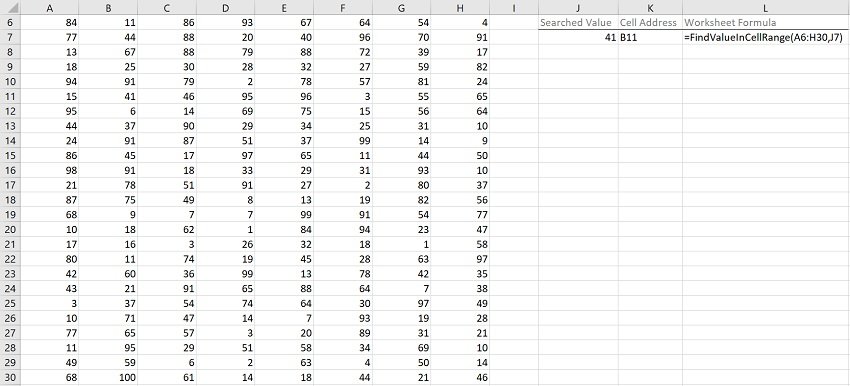
Macro Example to Find (Cell with) Value in Cell Range
The following macro (User-Defined Function) example does the following:
- Accepts two arguments:
- MyRange: The cell range you search in.
- MyValue: The numeric value you search for.
- Finds MyValue in MyRange.
- Returns a string containing the address (as an A1-style relative reference) of the first cell in the cell range (MyRange) where the numeric value (MyValue) is found.
Function FindValueInCellRange(MyRange As Range, MyValue As Variant) As String
    'Source: https://powerspreadsheets.com/
    'For further information: https://powerspreadsheets.com/excel-vba-find/

    'This UDF:
        '(1) Accepts 2 arguments: MyRange and MyValue
        '(2) Finds a value passed as argument (MyValue) in a cell range passed as argument (MyRange)
        '(3) Returns the address (as an A1-style relative reference) of the first cell in the cell range (MyRange) where the value (MyValue) is found

    With MyRange
        FindValueInCellRange = .Find(What:=MyValue, After:=.Cells(.Cells.Count), LookIn:=xlValues, LookAt:=xlWhole, SearchOrder:=xlByRows, SearchDirection:=xlNext).Address(RowAbsolute:=False, ColumnAbsolute:=False)
    End With

End Function
Effects of Executing Macro Example to Find (Cell with) Value in Cell Range
The following image illustrates the effects of using the macro (User-Defined Function) example. In this example:
- Columns A through H (cells A6 to H30) contain randomly generated values.
- Cell J7 contains the searched value (41).
- Cell K7 contains the worksheet formula that works with the macro (User-Defined Function) example. This worksheet formula returns the address (as an A1-style relative reference) of the first cell in the cell range (MyRange) where the numeric value (MyValue) is found. This is cell B11.
- Cell L7 displays the worksheet formula used in cell K7 (=FindValueInCellRange(A6:H30,J7)).
- The cell range where the search is carried out contains cells A6 to H30 (A6:H30).
- The searched value is stored in cell J7 (J7).
#2. Excel VBA Find (Cell with) Value in Table
VBA Code to Find (Cell with) Value in Table
To find a cell with a numeric value in an Excel Table, use the following structure/template in the applicable statement:
ListObjectObject.DataBodyRange.Find(What:=SearchedValue, After:=SingleCellRangeObject, LookIn:=xlValues, LookAt:=xlWhole, SearchOrder:=XlSearchOrderConstant, SearchDirection:=XlSearchDirectionConstant)
The following Sections describe the main elements in this structure.
ListObjectObject
A ListObject object representing the Excel Table you search in.
DataBodyRange
The ListObject.DataBodyRange property returns a Range object representing the cell range containing an Excel Table’s values (excluding the headers).
Find
The Range.Find method:
- Finds specific information (the numeric value you search for) in a cell range (containing the applicable Excel Table’s values).
- Returns a Range object representing the first cell where the information is found.
What:=SearchedValue
The What parameter of the Range.Find method specifies the data to search for.
To find a cell with a numeric value in an Excel Table, set the What parameter to the numeric value you search for (SearchedValue).
After:=SingleCellRangeObject
The After parameter of the Range.Find method specifies the cell after which the search begins. This must be a single cell in the cell range you search in (containing the applicable Excel Table’s values).
If you omit specifying the After parameter, the search begins after the first cell (in the upper left corner) of the cell range you search in (containing the applicable Excel Table’s values).
To find a cell with a numeric value in an Excel Table, set the After parameter to a Range object representing the cell after which the search begins.
LookIn:=xlValues
The LookIn parameter of the Range.Find method:
- Specifies the type of data to search in.
- Can take any of the built-in constants/values from the XlFindLookIn enumeration.
To find a cell with a numeric value in an Excel Table, set the LookIn parameter to xlValues. xlValues refers to values.
LookAt:=xlWhole
The LookAt parameter of the Range.Find method:
- Specifies against which of the following the data you are searching for is matched:
- The entire/whole searched cell contents.
- Any part of the searched cell contents.
- Can take any of the built-in constants/values from the XlLookAt enumeration.
To find a cell with a numeric value in an Excel Table, set the LookAt parameter to xlWhole. xlWhole matches the data you are searching for against the entire/whole searched cell contents.
SearchOrder:=XlSearchOrderConstant
The SearchOrder parameter of the Range.Find method:
- Specifies the order in which the applicable cell range (containing the applicable Excel Table’s values) is searched:
- By rows.
- By columns.
- Can take any of the built-in constants/values from the XlSearchOrder enumeration.
To find a cell with a numeric value in an Excel Table, set the SearchOrder parameter to either of the following, as applicable:
- xlByRows (SearchOrder:=xlByRows): To search by rows.
- xlByColumns (SearchOrder:=xlByColumns): To search by columns.
SearchDirection:=XlSearchDirectionConstant
The SearchDirection parameter of the Range.Find method:
- Specifies the search direction:
- Search for the previous match.
- Search for the next match.
- Can take any of the built-in constants/values from the XlSearchDirection enumeration.
To find a cell with a numeric value in an Excel Table, set the SearchDirection parameter to either of the following, as applicable:
- xlNext (SearchDirection:=xlNext): To search for the next match.
- xlPrevious (SearchDirection:=xlPrevious): To search for the previous match.
Macro Example to Find (Cell with) Value in Table
The following macro (User-Defined Function) example does the following:
- Accepts 3 arguments:
- MyWorksheetName: The name of the worksheet where the Excel Table you search in is stored.
- MyValue: The numeric value you search for.
- MyTableIndex: The index number of the Excel Table (stored in the worksheet named MyWorksheetName) you search in. MyTableIndex is an optional argument with a default value of 1.
- Finds MyValue in the applicable Excel Table’s values (excluding the headers).
- Returns a string containing the address (as an A1-style relative reference) of the first cell in the applicable Excel Table where the numeric value (MyValue) is found.
Function FindValueInTable(MyWorksheetName As String, MyValue As Variant, Optional MyTableIndex As Long = 1) As String
    'Source: https://powerspreadsheets.com/
    'For further information: https://powerspreadsheets.com/excel-vba-find/

    'This UDF:
        '(1) Accepts 3 arguments: MyWorksheetName, MyValue and MyTableIndex
        '(2) Finds a value passed as argument (MyValue) in an Excel Table stored in a worksheet whose name is passed as argument (MyWorksheetName). The index number of the Excel Table is either:
            '(1) Passed as an argument (MyTableIndex); or
            '(2) Assumed to be 1 (if MyTableIndex is omitted)
        '(3) Returns the address (as an A1-style relative reference) of the first cell in the Excel Table (stored in the MyWorksheetName worksheet and whose index is MyTableIndex) where the value (MyValue) is found

    With ThisWorkbook.Worksheets(MyWorksheetName).ListObjects(MyTableIndex).DataBodyRange
        FindValueInTable = .Find(What:=MyValue, After:=.Cells(.Cells.Count), LookIn:=xlValues, LookAt:=xlWhole, SearchOrder:=xlByRows, SearchDirection:=xlNext).Address(RowAbsolute:=False, ColumnAbsolute:=False)
    End With

End Function
Effects of Executing Macro Example to Find (Cell with) Value in Table
The following image illustrates the effects of using the macro (User-Defined Function) example. In this example:
- Columns A through H (cells A6 to H31) contain an Excel Table with randomly generated values.
- Cell J7 contains the searched value (41).
- Cell K7 contains the worksheet formula that works with the macro (User-Defined Function) example. This worksheet formula returns the address (as an A1-style relative reference) of the first cell in the Excel Table where the numeric value (MyValue) is found. This is cell B12.
- Cell L7 displays the worksheet formula used in cell K7 (=FindValueInTable(“Find Value in Table”,J7)).
- The name of the worksheet where the Excel Table is stored is “Find Value in Table” (“Find Value in Table”).
- The searched value is stored in cell J7 (J7).
- The index number of the Excel Table is 1 (by default).
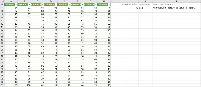
#3. Excel VBA Find (Cell with) Value in Column
VBA Code to Find (Cell with) Value in Column
To find a cell with a numeric value in a column, use the following structure/template in the applicable statement:
RangeObjectColumn.Find(What:=SearchedValue, After:=SingleCellRangeObject, LookIn:=xlValues, LookAt:=xlWhole, SearchOrder:=xlByRows, SearchDirection:=XlSearchDirectionConstant)
The following Sections describe the main elements in this structure.
RangeObjectColumn
A Range object representing the column you search in.
Find
The Range.Find method:
- Finds specific information (the numeric value you search for) in a cell range (RangeObjectColumn).
- Returns a Range object representing the first cell where the information is found.
What:=SearchedValue
The What parameter of the Range.Find method specifies the data to search for.
To find a cell with a numeric value in a column, set the What parameter to the numeric value you search for (SearchedValue).
After:=SingleCellRangeObject
The After parameter of the Range.Find method specifies the cell after which the search begins. This must be a single cell in the column you search in (RangeObjectColumn).
If you omit specifying the After parameter, the search begins after the first cell of the column you search in (RangeObjectColumn).
To find a cell with a numeric value in a column, set the After parameter to a Range object representing the cell after which the search begins.
LookIn:=xlValues
The LookIn parameter of the Range.Find method:
- Specifies the type of data to search in.
- Can take any of the built-in constants/values from the XlFindLookIn enumeration.
To find a cell with a numeric value in a column, set the LookIn parameter to xlValues. xlValues refers to values.
LookAt:=xlWhole
The LookAt parameter of the Range.Find method:
- Specifies against which of the following the data you are searching for is matched:
- The entire/whole searched cell contents.
- Any part of the searched cell contents.
- Can take any of the built-in constants/values from the XlLookAt enumeration.
To find a cell with a numeric value in a column, set the LookAt parameter to xlWhole. xlWhole matches the data you are searching for against the entire/whole searched cell contents.
SearchOrder:=xlByRows
The SearchOrder parameter of the Range.Find method:
- Specifies the order in which the applicable column (RangeObjectColumn) is searched:
- By rows.
- By columns.
- Can take any of the built-in constants/values from the XlSearchOrder enumeration.
To find a cell with a numeric value in a column, set the SearchOrder parameter to xlByRows. xlByRows results in the Range.Find method searching by rows.
SearchDirection:=XlSearchDirectionConstant
The SearchDirection parameter of the Range.Find method:
- Specifies the search direction:
- Search for the previous match.
- Search for the next match.
- Can take any of the built-in constants/values from the XlSearchDirection enumeration.
To find a cell with a numeric value in a column, set the SearchDirection parameter to either of the following, as applicable:
- xlNext (SearchDirection:=xlNext): To search for the next match.
- xlPrevious (SearchDirection:=xlPrevious): To search for the previous match.
Macro Example to Find (Cell with) Value in Column
The following macro (User-Defined Function) example does the following:
- Accepts two arguments:
- MyColumn: The column you search in.
- MyValue: The numeric value you search for.
- Finds MyValue in MyColumn.
- Returns a string containing the address (as an A1-style relative reference) of the first cell in the column (MyColumn) where the numeric value (MyValue) is found.
Function FindValueInColumn(MyColumn As Range, MyValue As Variant) As String
    'Source: https://powerspreadsheets.com/
    'For further information: https://powerspreadsheets.com/excel-vba-find/

    'This UDF:
        '(1) Accepts 2 arguments: MyColumn and MyValue
        '(2) Finds a value passed as argument (MyValue) in a column passed as argument (MyColumn)
        '(3) Returns the address (as an A1-style relative reference) of the first cell in the column (MyColumn) where the value (MyValue) is found

    With MyColumn
        FindValueInColumn = .Find(What:=MyValue, After:=.Cells(.Cells.Count), LookIn:=xlValues, LookAt:=xlWhole, SearchOrder:=xlByRows, SearchDirection:=xlNext).Address(RowAbsolute:=False, ColumnAbsolute:=False)
    End With

End Function
Effects of Executing Macro Example to Find (Cell with) Value in Column
The following image illustrates the effects of using the macro (User-Defined Function) example. In this example:
- Column A (cells A6 to A31) contains randomly generated values.
- Cell C7 contains the searched value (90).
- Cell D7 contains the worksheet formula that works with the macro (User-Defined Function) example. This worksheet formula returns the address (as an A1-style relative reference) of the first cell in the column (MyColumn) where the numeric value (MyValue) is found. This is cell A13.
- Cell E7 displays the worksheet formula used in cell D7 (=FindValueInColumn(A:A,C7)).
- The column where the search is carried out is column A (A:A).
- The searched value is stored in cell C7 (C7).
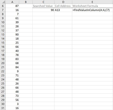
#4. Excel VBA Find (Cell with) Value in Table Column
VBA Code to Find (Cell with) Value in Table Column
To find a cell with a numeric value in an Excel Table column, use the following structure/template in the applicable statement:
ListColumnObject.DataBodyRange.Find(What:=SearchedValue, After:=SingleCellRangeObject, LookIn:=xlValues, LookAt:=xlWhole, SearchOrder:=XlSearchOrderConstant, SearchDirection:=XlSearchDirectionConstant)
The following Sections describe the main elements in this structure.
ListColumnObject
A ListColumn object representing the Excel Table column you search in.
DataBodyRange
The ListColumn.DataBodyRange property returns a Range object representing the cell range containing an Excel Table column’s values (excluding the header).
Find
The Range.Find method:
- Finds specific information (the numeric value you search for) in a cell range (containing the applicable Excel Table column’s values).
- Returns a Range object representing the first cell where the information is found.
What:=SearchedValue
The What parameter of the Range.Find method specifies the data to search for.
To find a cell with a numeric value in an Excel Table column, set the What parameter to the numeric value you search for (SearchedValue).
After:=SingleCellRangeObject
The After parameter of the Range.Find method specifies the cell after which the search begins. This must be a single cell in the cell range you search in (containing the applicable Excel Table column’s values).
If you omit specifying the After parameter, the search begins after the first cell of the cell range you search in (containing the applicable Excel Table column’s values).
To find a cell with a numeric value in an Excel Table column, set the After parameter to a Range object representing the cell after which the search begins.
LookIn:=xlValues
The LookIn parameter of the Range.Find method:
- Specifies the type of data to search in.
- Can take any of the built-in constants/values from the XlFindLookIn enumeration.
To find a cell with a numeric value in an Excel Table column, set the LookIn parameter to xlValues. xlValues refers to values.
LookAt:=xlWhole
The LookAt parameter of the Range.Find method:
- Specifies against which of the following the data you are searching for is matched:
- The entire/whole searched cell contents.
- Any part of the searched cell contents.
- Can take any of the built-in constants/values from the XlLookAt enumeration.
To find a cell with a numeric value in an Excel Table column, set the LookAt parameter to xlWhole. xlWhole matches the data you are searching for against the entire/whole searched cell contents.
SearchOrder:=XlSearchOrderConstant
The SearchOrder parameter of the Range.Find method:
- Specifies the order in which the applicable cell range (containing the applicable Excel Table column’s values) is searched:
- By rows.
- By columns.
- Can take any of the built-in constants/values from the XlSearchOrder enumeration.
To find a cell with a numeric value in an Excel Table column, set the SearchOrder parameter to either of the following, as applicable:
- xlByRows (SearchOrder:=xlByRows): To search by rows.
- xlByColumns (SearchOrder:=xlByColumns): To search by columns.
SearchDirection:=XlSearchDirectionConstant
The SearchDirection parameter of the Range.Find method:
- Specifies the search direction:
- Search for the previous match.
- Search for the next match.
- Can take any of the built-in constants/values from the XlSearchDirection enumeration.
To find a cell with a numeric value in an Excel Table column, set the SearchDirection parameter to either of the following, as applicable:
- xlNext (SearchDirection:=xlNext): To search for the next match.
- xlPrevious (SearchDirection:=xlPrevious): To search for the previous match.
Macro Example to Find (Cell with) Value in Table Column
The following macro (User-Defined Function) example does the following:
- Accepts 4 arguments:
- MyWorksheetName: The name of the worksheet where the Excel Table (containing the column you search in) is stored.
- MyColumnIndex: The index/column number of the column you search in (in the applicable Excel Table).
- MyValue: The numeric value you search for.
- MyTableIndex: The index number of the Excel Table (stored in the worksheet named MyWorksheetName) containing the column you search in. MyTableIndex is an optional argument with a default value of 1.
- Finds MyValue in the applicable Excel Table column’s values (excluding the header).
- Returns a string containing the address (as an A1-style relative reference) of the first cell in the applicable Excel Table column where the numeric value (MyValue) is found.
Function FindValueInTableColumn(MyWorksheetName As String, MyColumnIndex As Long, MyValue As Variant, Optional MyTableIndex As Long = 1) As String
    'Source: https://powerspreadsheets.com/
    'For further information: https://powerspreadsheets.com/excel-vba-find/

    'This UDF:
        '(1) Accepts 4 arguments: MyWorksheetName, MyColumnIndex, MyValue and MyTableIndex
        '(2) Finds a value passed as argument (MyValue) in an Excel Table column, where:
            '(1) The table column's index is passed as argument (MyColumnIndex); and
            '(2) The Excel Table is stored in a worksheet whose name is passed as argument (MyWorksheetName). The index number of the Excel Table is either:
                '(1) Passed as an argument (MyTableIndex); or
                '(2) Assumed to be 1 (if MyTableIndex is omitted)
        '(3) Returns the address (as an A1-style relative reference) of the first cell in the applicable Excel Table column where the value (MyValue) is found

    With ThisWorkbook.Worksheets(MyWorksheetName).ListObjects(MyTableIndex).ListColumns(MyColumnIndex).DataBodyRange
        FindValueInTableColumn = .Find(What:=MyValue, After:=.Cells(.Cells.Count), LookIn:=xlValues, LookAt:=xlWhole, SearchOrder:=xlByRows, SearchDirection:=xlNext).Address(RowAbsolute:=False, ColumnAbsolute:=False)
    End With

End Function
Effects of Executing Macro Example to Find (Cell with) Value in Table Column
The following image illustrates the effects of using the macro (User-Defined Function) example. In this example:
- Columns A through H (cells A6 to H31) contain an Excel Table with randomly generated values. Cells in the first row (row 7) contain the searched value (90), except for the cell in the searched column (Column 3).
- Cell J7 contains the searched value (90).
- Cell K7 contains the worksheet formula that works with the macro (User-Defined Function) example. This worksheet formula returns the address (as an A1-style relative reference) of the first cell in the applicable Excel Table column (Column 3) where the numeric value (MyValue) is found. This is cell C14.
- Cell L7 displays the worksheet formula used in cell K7 (=FindValueInTableColumn(“Find Value in Table Column”,3, J7)).
- The name of the worksheet where the Excel Table is stored is “Find Value in Table Column” (“Find Value in Table Column”).
- The index number of the Excel Table column is 3 (3).
- The searched value is stored in cell J7 (J7).
- The index number of the Excel Table is 1 (by default).
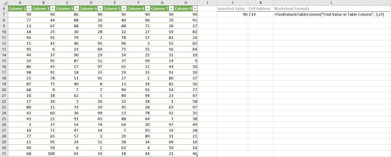
#5. Excel VBA Find Minimum Value in Cell Range
VBA Code to Find Minimum Value in Cell Range
To find the minimum value in a cell range, use the following structure/template in the applicable statement:
Application.Min(CellRangeObject)
The following Sections describe the main elements in this structure.
Application.Min
The WorksheetFunction.Min method returns the minimum value in a set of values.
CellRangeObject
The WorksheetFunction.Min method accepts up to thirty parameters (Arg1 to Arg30). These are the values for which you want to find the minimum value.
To find the minimum value in a cell range, pass a Range object (CellRangeObject) representing the cell range whose minimum value you want to find as method parameter.
Macro Example to Find Minimum Value in Cell Range
The following macro (User-Defined Function) example does the following:
- Accepts 1 argument (MyRange): The cell range whose minimum value you search for.
- Finds and returns the minimum value in the cell range (MyRange).
Function FindMinimumValueInCellRange(MyRange As Range) As Double
    'Source: https://powerspreadsheets.com/
    'For further information: https://powerspreadsheets.com/excel-vba-find/

    'This UDF:
        '(1) Accepts 1 argument: MyRange
        '(2) Finds the minimum value in the cell range passed as argument (MyRange)

    FindMinimumValueInCellRange = Application.Min(MyRange)

End Function
Effects of Executing Macro Example to Find Minimum Value in Cell Range
The following image illustrates the effects of using the macro (User-Defined Function) example. In this example:
- Columns A through H (cells A6 to H30) contain randomly generated values.
- Cell J7 contains the worksheet formula that works with the macro (User-Defined Function) example. This worksheet formula returns the minimum value in the cell range (MyRange). This is the number 1.
- Cell K7 displays the worksheet formula used in cell J7 (=FindMinimumValueInCellRange(A6:H30)). The cell range where the search is carried out contains cells A6 to H30 (A6:H30).
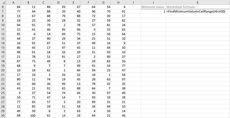
#6. Excel VBA Find (Cell with) String (or Text) in Cell Range
VBA Code to Find (Cell with) String (or Text) in Cell Range
To find a cell with a string (or text) in a cell range, use the following structure/template in the applicable statement:
CellRangeObject.Find(What:=SearchedString, After:=SingleCellRangeObject, LookIn:=XlFindLookInConstant, LookAt:=XlLookAtConstant, SearchOrder:=XlSearchOrderConstant, SearchDirection:=XlSearchDirectionConstant, MatchCase:=BooleanValue)
The following Sections describe the main elements in this structure.
CellRangeObject
A Range object representing the cell range you search in.
Find
The Range.Find method:
- Finds specific information (the string or text you search for) in a cell range (CellRangeObject).
- Returns a Range object representing the first cell where the information is found.
What:=SearchedString
The What parameter of the Range.Find method specifies the data to search for.
To find a cell with a string (or text) in a cell range, set the What parameter to the string (or text) you search for (SearchedString).
After:=SingleCellRangeObject
The After parameter of the Range.Find method specifies the cell after which the search begins. This must be a single cell in the cell range you search in (CellRangeObject).
If you omit specifying the After parameter, the search begins after the first cell (in the upper left corner) of the cell range you search in (CellRangeObject).
To find a cell with a string (or text) in a cell range, set the After parameter to a Range object representing the cell after which the search begins.
LookIn:=XlFindLookInConstant
The LookIn parameter of the Range.Find method:
- Specifies the type of data to search in.
- Can take any of the built-in constants/values from the XlFindLookIn enumeration.
To find a cell with a string (or text) in a cell range, set the LookIn parameter to either of the following, as applicable:
- xlFormulas (LookIn:=xlFormulas): To search in the applicable cell range’s formulas.
- xlValues (LookIn:=xlValues): To search in the applicable cell range’s values.
LookAt:=XlLookAtConstant
The LookAt parameter of the Range.Find method:
- Specifies against which of the following the data you are searching for is matched:
- The entire/whole searched cell contents.
- Any part of the searched cell contents.
- Can take any of the built-in constants/values from the XlLookAt enumeration.
To find a cell with a string (or text) in a cell range, set the LookAt parameter to either of the following, as applicable:
- xlWhole (LookAt:=xlWhole): To match against the entire/whole searched cell contents.
- xlPart (LookAt:=xlPart): To match against any part of the searched cell contents.
SearchOrder:=XlSearchOrderConstant
The SearchOrder parameter of the Range.Find method:
- Specifies the order in which the applicable cell range (CellRangeObject) is searched:
- By rows.
- By columns.
- Can take any of the built-in constants/values from the XlSearchOrder enumeration.
To find a cell with a string (or text) in a cell range, set the SearchOrder parameter to either of the following, as applicable:
- xlByRows (SearchOrder:=xlByRows): To search by rows.
- xlByColumns (SearchOrder:=xlByColumns): To search by columns.
SearchDirection:=XlSearchDirectionConstant
The SearchDirection parameter of the Range.Find method:
- Specifies the search direction:
- Search for the previous match.
- Search for the next match.
- Can take any of the built-in constants/values from the XlSearchDirection enumeration.
To find a cell with a string (or text) in a cell range, set the SearchDirection parameter to either of the following, as applicable:
- xlNext (SearchDirection:=xlNext): To search for the next match.
- xlPrevious (SearchDirection:=xlPrevious): To search for the previous match.
MatchCase:=BooleanValue
The MatchCase parameter of the Range.Find method specifies whether the search is:
- Case-sensitive; or
- Case-insensitive.
The default value of the MatchCase parameter is False.
To find a cell with a string (or text) in a cell range, set the MatchCase parameter to either of the following, as applicable:
- True (MatchCase:=True): To carry out a case-sensitive search.
- False (MatchCase:=False): To carry out a case-insensitive search.
Macro Example to Find (Cell with) String (or Text) in Cell Range
The following macro (User-Defined Function) example does the following:
- Accepts two arguments:
- MyRange: The cell range you search in.
- MyString: The string (or text) you search for.
- Finds MyString in MyRange. The search is case-insensitive.
- Returns a string containing the address (as an A1-style relative reference) of the first cell in the cell range (MyRange) where the string or text (MyString) is found.
Function FindStringInCellRange(MyRange As Range, MyString As Variant) As String
    'Source: https://powerspreadsheets.com/
    'For further information: https://powerspreadsheets.com/excel-vba-find/

    'This UDF:
        '(1) Accepts 2 arguments: MyRange and MyString
        '(2) Finds a string passed as argument (MyString) in a cell range passed as argument (MyRange). The search is case-insensitive
        '(3) Returns the address (as an A1-style relative reference) of the first cell in the cell range (MyRange) where the string (MyString) is found

    With MyRange
        FindStringInCellRange = .Find(What:=MyString, After:=.Cells(.Cells.Count), LookIn:=xlValues, LookAt:=xlWhole, SearchOrder:=xlByRows, SearchDirection:=xlNext, MatchCase:=False).Address(RowAbsolute:=False, ColumnAbsolute:=False)
    End With

End Function
Effects of Executing Macro Example to Find (Cell with) String (or Text) in Cell Range
The following image illustrates the effects of using the macro (User-Defined Function) example. In this example:
- Columns A through H (cells A6 to H30) contain randomly generated words.
- Cell J7 contains the searched string or text (Excel).
- Cell K7 contains the worksheet formula that works with the macro (User-Defined Function) example. This worksheet formula returns the address (as an A1-style relative reference) of the first cell in the cell range (MyRange) where the string or text (MyString) is found. This is cell F20.
- Cell L7 displays the worksheet formula used in cell K7 (=FindStringInCellRange(A6:H30,J7)).
- The cell range where the search is carried out contains cells A6 to H30 (A6:H30).
- The searched string or text is stored in cell J7 (J7).

#7. Excel VBA Find (Cell with) String (or Text) in Column
VBA Code to Find (Cell with) String (or Text) in Column
To find a cell with a string (or text) in a column, use the following structure/template in the applicable statement:
RangeObjectColumn.Find(What:=SearchedString, After:=SingleCellRangeObject, LookIn:=XlFindLookInConstant, LookAt:=XlLookAtConstant, SearchOrder:=xlByRows, SearchDirection:=XlSearchDirectionConstant, MatchCase:=BooleanValue)
The following Sections describe the main elements in this structure.
RangeObjectColumn
A Range object representing the column you search in.
Find
The Range.Find method:
- Finds specific information (the string or text you search for) in a cell range (RangeObjectColumn).
- Returns a Range object representing the first cell where the information is found.
What:=SearchedString
The What parameter of the Range.Find method specifies the data to search for.
To find a cell with a string (or text) in a column, set the What parameter to the string (or text) you search for (SearchedString).
After:=SingleCellRangeObject
The After parameter of the Range.Find method specifies the cell after which the search begins. This must be a single cell in the column you search in (RangeObjectColumn).
If you omit specifying the After parameter, the search begins after the first cell of the column you search in (RangeObjectColumn).
To find a cell with a string (or text) in a column, set the After parameter to a Range object representing the cell after which the search begins.
LookIn:=XlFindLookInConstant
The LookIn parameter of the Range.Find method:
- Specifies the type of data to search in.
- Can take any of the built-in constants/values from the XlFindLookIn enumeration.
To find a cell with a string (or text) in a column, set the LookIn parameter to either of the following, as applicable:
- xlFormulas (LookIn:=xlFormulas): To search in the applicable column’s formulas.
- xlValues (LookIn:=xlValues): To search in the applicable column’s values.
LookAt:=XlLookAtConstant
The LookAt parameter of the Range.Find method:
- Specifies against which of the following the data you are searching for is matched:
- The entire/whole searched cell contents.
- Any part of the searched cell contents.
- Can take any of the built-in constants/values from the XlLookAt enumeration.
To find a cell with a string (or text) in a column, set the LookAt parameter to either of the following, as applicable:
- xlWhole (LookAt:=xlWhole): To match against the entire/whole searched cell contents.
- xlPart (LookAt:=xlPart): To match against any part of the searched cell contents.
SearchOrder:=xlByRows
The SearchOrder parameter of the Range.Find method:
- Specifies the order in which the applicable column (RangeObjectColumn) is searched:
- By rows.
- By columns.
- Can take any of the built-in constants/values from the XlSearchOrder enumeration.
To find a cell with a string (or text) in a column, set the SearchOrder parameter to xlByRows. xlByRows results in the Range.Find method searching by rows.
SearchDirection:=XlSearchDirectionConstant
The SearchDirection parameter of the Range.Find method:
- Specifies the search direction:
- Search for the previous match.
- Search for the next match.
- Can take any of the built-in constants/values from the XlSearchDirection enumeration.
To find a cell with a string (or text) in a column, set the SearchDirection parameter to either of the following, as applicable:
- xlNext (SearchDirection:=xlNext): To search for the next match.
- xlPrevious (SearchDirection:=xlPrevious): To search for the previous match.
MatchCase:=BooleanValue
The MatchCase parameter of the Range.Find method specifies whether the search is:
- Case-sensitive; or
- Case-insensitive.
The default value of the MatchCase parameter is False.
To find a cell with a string (or text) in a column, set the MatchCase parameter to either of the following, as applicable:
- True (MatchCase:=True): To carry out a case-sensitive search.
- False (MatchCase:=False): To carry out a case-insensitive search.
Macro Example to Find (Cell with) String (or Text) in Column
The following macro (User-Defined Function) example does the following:
- Accepts two arguments:
- MyColumn: The column you search in.
- MyString: The string (or text) you search for.
- Finds MyString in MyColumn. The search is case-insensitive.
- Returns a string containing the address (as an A1-style relative reference) of the first cell in the column (MyColumn) where the string or text (MyString) is found.
Function FindStringInColumn(MyColumn As Range, MyString As Variant) As String
    'Source: https://powerspreadsheets.com/
    'For further information: https://powerspreadsheets.com/excel-vba-find/

    'This UDF:
        '(1) Accepts 2 arguments: MyColumn and MyString
        '(2) Finds a string passed as argument (MyString) in a column passed as argument (MyColumn). The search is case-insensitive
        '(3) Returns the address (as an A1-style relative reference) of the first cell in the column (MyColumn) where the string (MyString) is found

    With MyColumn
        FindStringInColumn = .Find(What:=MyString, After:=.Cells(.Cells.Count), LookIn:=xlValues, LookAt:=xlWhole, SearchOrder:=xlByRows, SearchDirection:=xlNext, MatchCase:=False).Address(RowAbsolute:=False, ColumnAbsolute:=False)
    End With

End Function
Effects of Executing Macro Example to Find (Cell with) String (or Text) in Column
The following image illustrates the effects of using the macro (User-Defined Function) example. In this example:
- Column A (cells A6 to A30) contains randomly generated words.
- Cell C7 contains the searched string or text (Excel).
- Cell D7 contains the worksheet formula that works with the macro (User-Defined Function) example. This worksheet formula returns the address (as an A1-style relative reference) of the first cell in the column (MyColumn) where the string or text (MyString) is found. This is cell A21.
- Cell E7 displays the worksheet formula used in cell D7 (=FindStringInColumn(A:A,C7)).
- The column where the search is carried out is column A (A:A).
- The searched string or text is stored in cell C7 (C7).

#8. Excel VBA Find String (or Text) in Cell
VBA Code to Find String (or Text) in Cell
To find a string (or text) in a cell, use the following structure/template in the applicable statement:
InStr(StartingPosition, SearchedCell.Value, SearchedString, VbCompareMethodConstant)
The following Sections describe the main elements in this structure.
InStr
The InStr function returns a number. This number specifies the position of the first occurrence of a string or text (SearchedString) in another string (the string stored in SearchedCell).
StartingPosition
The Start argument of the InStr function is:
- An optional argument.
- A numeric expression specifying the starting position for the string (or text) search.
If you omit specifying the Start argument, the search begins at the first character of the searched string (the string stored in SearchedCell).
To find a string (or text) in a cell, set the Start argument to the position (in the string stored in SearchedCell) where the string (or text) search starts.
SearchedCell.Value
The String1 argument of the InStr function represents the string expression the InStr function searches in.
To find a string (or text) in a cell, set the String1 argument to the value/string stored in the searched cell. For these purposes:
- “SearchedCell” is a Range object representing the searched cell.
- “Value” refers to the Range.Value property. The Range.Value property returns the value/string stored in the searched cell (SearchedCell).
SearchedString
The String2 argument of the InStr function represents the string expression (or text) the InStr function searches for.
To find a string (or text) in a cell, set the String2 argument to the string (or text) you search for.
VbCompareMethodConstant
The Compare argument of the InStr function:
- Is an optional argument.
- Specifies the type of string comparison carried out by the InStr function.
- Can take any of the built-in constants/values from the vbCompareMethod enumeration.
If you omit specifying the Compare argument, the type of string comparison is determined by the Option Compare statement. The Option Compare statement declares the default string comparison method at a module level. The default string comparison method is binary (vbBinaryCompare).
To find a string (or text) in a cell, set the Compare argument to either of the following, as applicable:
- vbBinaryCompare: Performs a binary comparison. vbBinaryCompare:
- Results in a case-sensitive search.
- May be (slightly) faster than vbTextCompare.
- vbTextCompare: Performs a textual comparison. vbTextCompare:
- Results in a case-insensitive search.
- May be (slightly) slower than vbBinaryCompare.
- Is more prone to errors/bugs than vbBinaryCompare.
Macro Example to Find String (or Text) in Cell
The following macro (User-Defined Function) example does the following:
- Accepts three arguments:
- MyCell: The cell you search in.
- MyString: The string (or text) you search for.
- MyStartingPosition: The starting position for the string (or text) search. MyStartingPosition is an optional argument with a default value of 1.
- Finds MyString in the value/string stored in MyCell.
- Returns the following:
- If MyString is not found in the value/string stored in MyCell, the string “String not found in cell”.
- If MyString is found in the value/string stored in MyCell, the position of the first occurrence of MyString in the value/string stored in MyCell.
Function FindStringInCell(MyCell As Range, MyString As Variant, Optional MyStartingPosition As Variant = 1) As Variant
    'Source: https://powerspreadsheets.com/
    'For further information: https://powerspreadsheets.com/excel-vba-find/

    'This UDF:
        '(1) Accepts three arguments: MyCell, MyString and MyStartingPosition (optional argument with a default value of 1)
        '(2) Finds a string passed as argument (MyString) in the value/string stored in a cell passed as argument (MyCell)
        '(3) Returns the following (as applicable):
            'If MyString is not found in the value/string stored in MyCell: The string "String not found in cell"
            'If MyString is found in the value/string stored in MyCell: The position of the first occurrence of MyString in the value/string stored in MyCell

    'Obtain position of first occurrence of MyString in the value/string stored in MyCell
    FindStringInCell = InStr(MyStartingPosition, MyCell.Value, MyString, vbBinaryCompare)

    'If MyString is not found in the value/string stored in MyCell, return the string "String not found in cell"
    If FindStringInCell = 0 Then FindStringInCell = "String not found in cell"

End Function
Effects of Executing Macro Example to Find String (or Text) in Cell
The following image illustrates the effects of using the macro (User-Defined Function) example. In this example:
- Column A (cells A7 to A31) contains randomly generated words.
- Column B (cells B7 to B31) contains a 2-character string (ar).
- Column C (cells C7 to C31) contains worksheet formulas working with the macro (User-Defined Function) example. These worksheet formulas return either of the following (as applicable):
- The string “String not found in cell”, if the string (or text) specified in the applicable cell of column B is not found in the applicable cell of column A.
- The position of the first occurrence of the string (or text) specified in the applicable cell of column B in the applicable cell of column A, if the string (or text) specified in the applicable cell of column B is found in the applicable cell of column A.
- Column D (cells D7 to D31) displays the worksheet formulas used in column C (=FindStringInCell(CellInColumnA,CellInColumnB)).
- The cell where the search is carried out is in column A (CellInColumnA).
- The searched string or text is stored in column B (CellInColumnB).

#9. Excel VBA Find String (or Text) in String
VBA Code to Find String (or Text) in String
To find a string (or text) in a string, use the following structure/template in the applicable statement:
InStr(StartingPosition, SearchedString, SearchedText, VbCompareMethodConstant)
The following Sections describe the main elements in this structure.
InStr
The InStr function returns a number. This number specifies the position of the first occurrence of a string or text (SearchedText) in another string (SearchedString).
StartingPosition
The Start argument of the InStr function is:
- An optional argument.
- A numeric expression specifying the starting position for the string (or text) search.
If you omit specifying the Start argument, the search begins at the first character of the searched string (SearchedString).
To find a string (or text) in a string, set the Start argument to the position (in SearchedString) where the string (or text) search starts.
SearchedString
The String1 argument of the InStr function represents the string expression the InStr function searches in.
To find a string (or text) in a string, set the String1 argument to the searched string.
SearchedText
The String2 argument of the InStr function represents the string expression (or text) the InStr function searches for.
To find a string (or text) in a string, set the String2 argument to the string (or text) you search for.
VbCompareMethodConstant
The Compare argument of the InStr function:
- Is an optional argument.
- Specifies the type of string comparison carried out by the InStr function.
- Can take any of the built-in constants/values from the vbCompareMethod enumeration.
If you omit specifying the Compare argument, the type of string comparison is determined by the Option Compare statement. The Option Compare statement declares the default string comparison method at a module level. The default string comparison method is binary (vbBinaryCompare).
To find a string (or text) in a string, set the Compare argument to either of the following, as applicable:
- vbBinaryCompare: Performs a binary comparison. vbBinaryCompare:
- Results in a case-sensitive search.
- May be (slightly) faster than vbTextCompare.
- vbTextCompare: Performs a textual comparison. vbTextCompare:
- Results in a case-insensitive search.
- May be (slightly) slower than vbBinaryCompare.
- Is more prone to errors/bugs than vbBinaryCompare.
Macro Example to Find String (or Text) in String
The following macro (User-Defined Function) example does the following:
- Accepts three arguments:
- MyString: The string you search in.
- MyText: The string (or text) you search for.
- MyStartingPosition: The starting position for the string (or text) search. MyStartingPosition is an optional argument with a default value of 1.
- Finds MyText in MyString.
- Returns the following:
- If MyText is not found in MyString, the string “Text not found in string”.
- If MyText is found in MyString, the position of the first occurrence of MyText in MyString.
Function FindTextInString(MyString As Variant, MyText As Variant, Optional MyStartingPosition As Variant = 1) As Variant
    'Source: https://powerspreadsheets.com/
    'For further information: https://powerspreadsheets.com/excel-vba-find/

    'This UDF:
        '(1) Accepts three arguments: MyString, MyText and MyStartingPosition (optional argument with a default value of 1)
        '(2) Finds text (a string) passed as argument (MyText) in a string passed as argument (MyString)
        '(3) Returns the following (as applicable):
            'If MyText is not found in MyString: The string "Text not found in string"
            'If MyText is found in MyString: The position of the first occurrence of MyText in MyString

    'Obtain position of first occurrence of MyText in MyString
    FindTextInString = InStr(MyStartingPosition, MyString, MyText, vbBinaryCompare)

    'If MyText is not found in MyString, return the string "Text not found in string"
    If FindTextInString = 0 Then FindTextInString = "Text not found in string"

End Function
Effects of Executing Macro Example to Find String (or Text) in String
The following image illustrates the effects of using the macro (User-Defined Function) example. In this example:
- Column A (cells A7 to A31) contains randomly generated words.
- Column B (cells B7 to B31) contains text (at).
- Column C (cells C7 to C31) contains worksheet formulas working with the macro (User-Defined Function) example. These worksheet formulas return either of the following (as applicable):
- The string “Text not found in string”, if the string (or text) specified in the applicable cell of column B is not found in the string specified in the applicable cell of column A.
- The position of the first occurrence of the string (or text) specified in the applicable cell of column B in the string specified in the applicable cell of column A, if the string (or text) specified in the applicable cell of column B is found in the string specified in the applicable cell of column A.
- Column D (cells D7 to D31) displays the worksheet formulas used in column C (=FindTextInString(CellInColumnA,CellInColumnB)).
- The string where the search is carried out is stored in column A (CellInColumnA).
- The searched string (or text) is stored in column B (CellInColumnB).
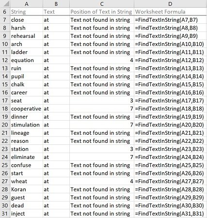
#10. Excel VBA Find Character in String
VBA Code to Find Character in String
To find a character in a string, use the following structure/template in the applicable statement:
InStr(StartingPosition, SearchedString, SearchedCharacter, VbCompareMethodConstant)
The following Sections describe the main elements in this structure.
InStr
The InStr function returns a number. This number specifies the position of the first occurrence of a string or text (SearchedCharacter) in another string (SearchedString).
StartingPosition
The Start argument of the InStr function is:
- An optional argument.
- A numeric expression specifying the starting position for the character search.
If you omit specifying the Start argument, the search begins at the first character of the searched string (SearchedString).
To find a character in a string, set the Start argument to the position (in SearchedString) where the character search starts.
SearchedString
The String1 argument of the InStr function represents the string expression the InStr function searches in.
To find a character in a string, set the String1 argument to the searched string.
SearchedCharacter
The String2 argument of the InStr function represents the string expression (or text) the InStr function searches for.
To find a character in a string, set the String2 argument to the character you search for.
VbCompareMethodConstant
The Compare argument of the InStr function:
- Is an optional argument.
- Specifies the type of string comparison carried out by the InStr function.
- Can take any of the built-in constants/values from the vbCompareMethod enumeration.
If you omit specifying the Compare argument, the type of string comparison is determined by the Option Compare statement. The Option Compare statement declares the default string comparison method at a module level. The default string comparison method is binary (vbBinaryCompare).
To find a character in a string, set the Compare argument to either of the following, as applicable:
- vbBinaryCompare: Performs a binary comparison. vbBinaryCompare:
- Results in a case-sensitive search.
- May be (slightly) faster than vbTextCompare.
- vbTextCompare: Performs a textual comparison. vbTextCompare:
- Results in a case-insensitive search.
- May be (slightly) slower than vbBinaryCompare.
- Is more prone to errors/bugs than vbBinaryCompare.
Macro Example to Find Character in String
The following macro (User-Defined Function) example does the following:
- Accepts three arguments:
- MyString: The string you search in.
- MyCharacter: The character you search for.
- MyStartingPosition: The starting position for the character search. MyStartingPosition is an optional argument with a default value of 1.
- Finds MyCharacter in MyString.
- Returns the following:
- If MyCharacter is not found in MyString, the string “Character not found in string”.
- If MyCharacter is found in MyString, the position of the first occurrence of MyCharacter in MyString.
Function FindCharacterInString(MyString As Variant, MyCharacter As Variant, Optional MyStartingPosition As Variant = 1) As Variant
    'Source: https://powerspreadsheets.com/
    'For further information: https://powerspreadsheets.com/excel-vba-find/

    'This UDF:
        '(1) Accepts three arguments: MyString, MyCharacter and MyStartingPosition (optional argument with a default value of 1)
        '(2) Finds a character passed as argument (MyCharacter) in a string passed as argument (MyString)
        '(3) Returns the following (as applicable):
            'If MyCharacter is not found in MyString: The string "Character not found in string"
            'If MyCharacter is found in MyString: The position of the first occurrence of MyCharacter in MyString

    'Obtain position of first occurrence of MyCharacter in MyString
    FindCharacterInString = InStr(MyStartingPosition, MyString, MyCharacter, vbBinaryCompare)

    'If MyCharacter is not found in MyString, return the string "Character not found in string"
    If FindCharacterInString = 0 Then FindCharacterInString = "Character not found in string"

End Function
Effects of Executing Macro Example to Find Character in String
The following image illustrates the effects of using the macro (User-Defined Function) example. In this example:
- Column A (cells A7 to A31) contains randomly generated words.
- Column B (cells B7 to B31) contains a character (a).
- Column C (cells C7 to C31) contains worksheet formulas working with the macro (User-Defined Function) example. These worksheet formulas return either of the following (as applicable):
- The string “Character not found in string”, if the character specified in the applicable cell of column B is not found in the string specified in the applicable cell of column A.
- The position of the first occurrence of the character specified in the applicable cell of column B in the string specified in the applicable cell of column A, if the character specified in the applicable cell of column B is found in the string specified in the applicable cell of column A.
- Column D (cells D7 to D31) displays the worksheet formulas used in column C (=FindCharacterInString(CellInColumnA,CellInColumnB)).
- The string where the search is carried out is stored in column A (CellInColumnA).
- The searched character is stored in column B (CellInColumnB).

#11. Excel VBA Find Column with Specific Header
VBA Code to Find Column with Specific Header
To find a column with a specific header, use the following structure/template in the applicable statement:
HeaderRowRangeObject.Find(What:=SearchedHeader, After:=SingleCellRangeObject, LookIn:=xlValues, LookAt:=xlWhole, SearchOrder:=xlByColumns, SearchDirection:=XlSearchDirectionConstant, MatchCase:=BooleanValue)
The following Sections describe the main elements in this structure.
HeaderRowRangeObject
A Range object representing the cell range containing the headers you search in.
Find
The Range.Find method:
- Finds specific information (the header you search for) in a cell range (HeaderRowRangeObject).
- Returns a Range object representing the first cell where the information is found.
What:=SearchedHeader
The What parameter of the Range.Find method specifies the data to search for.
To find a column with a specific header, set the What parameter to the header you search for (SearchedHeader).
After:=SingleCellRangeObject
The After parameter of the Range.Find method specifies the cell after which the search begins. This must be a single cell in the cell range containing the headers you search in (HeaderRowRangeObject).
If you omit specifying the After parameter, the search begins after the first cell of the cell range you search in (HeaderRowRangeObject).
To find a column with a specific header, set the After parameter to a Range object representing the cell after which the search begins.
LookIn:=xlValues
The LookIn parameter of the Range.Find method:
- Specifies the type of data to search in.
- Can take any of the built-in constants/values from the XlFindLookIn enumeration.
To find a column with a specific header, set the LookIn parameter to xlValues. xlValues refers to values.
LookAt:=xlWhole
The LookAt parameter of the Range.Find method:
- Specifies against which of the following the data you are searching for is matched:
- The entire/whole searched cell contents.
- Any part of the searched cell contents.
- Can take any of the built-in constants/values from the XlLookAt enumeration.
To find a column with a specific header, set the LookAt parameter to xlWhole. xlWhole matches the data you are searching for against the entire/whole searched cell contents.
SearchOrder:=xlByColumns
The SearchOrder parameter of the Range.Find method:
- Specifies the order in which the applicable cell range (HeaderRowRangeObject) is searched:
- By rows.
- By columns.
- Can take any of the built-in constants/values from the XlSearchOrder enumeration.
To find a column with a specific header, set the SearchOrder parameter to xlByColumns. xlByColumns searches by columns.
SearchDirection:=XlSearchDirectionConstant
The SearchDirection parameter of the Range.Find method:
- Specifies the search direction:
- Search for the previous match.
- Search for the next match.
- Can take any of the built-in constants/values from the XlSearchDirection enumeration.
To find a column with a specific header, set the SearchDirection parameter to either of the following, as applicable:
- xlNext (SearchDirection:=xlNext): To search for the next match.
- xlPrevious (SearchDirection:=xlPrevious): To search for the previous match.
MatchCase:=BooleanValue
The MatchCase parameter of the Range.Find method specifies whether the search is:
- Case-sensitive; or
- Case-insensitive.
The default value of the MatchCase parameter is False.
To find a column with a specific header, set the MatchCase parameter to either of the following, as applicable:
- True (MatchCase:=True): To carry out a case-sensitive search.
- False (MatchCase:=False): To carry out a case-insensitive search.
Macro Example to Find Column with Specific Header
The following macro (User-Defined Function) example does the following:
- Accepts two arguments:
- MyRange: The cell range whose first row contains the headers you search in.
- MyHeader: The header you search for.
- Finds MyHeader in the first row of MyRange.
- Returns the number of the column containing the first cell in the header row where the header (MyHeader) is found.
Function FindColumnWithSpecificHeader(MyRange As Range, MyHeader As Variant) As Long
    'Source: https://powerspreadsheets.com/
    'For further information: https://powerspreadsheets.com/excel-vba-find/

    'This UDF:
        '(1) Accepts 2 arguments: MyRange and MyHeader
        '(2) Finds a header passed as argument (MyHeader) in the first row (the header row) of a cell range passed as argument (MyRange). The search is case-insensitive
        '(3) Returns the number of the column containing the first cell in the header row where the header (MyHeader) is found

    With MyRange.Rows(1)
        FindColumnWithSpecificHeader = .Find(What:=MyHeader, After:=.Cells(.Cells.Count), LookIn:=xlValues, LookAt:=xlWhole, SearchOrder:=xlByColumns, SearchDirection:=xlNext, MatchCase:=False).Column
    End With

End Function
Effects of Executing Macro Example to Find Column with Specific Header
The following image illustrates the effects of using the macro (User-Defined Function) example. In this example:
- Columns A through H (cells A6 to H31) contain data with the following characteristics:
- Headers in its first row (row 6).
- Randomly generated values.
- Cell J7 contains the searched header (Column 3).
- Cell K7 contains the worksheet formula that works with the macro (User-Defined Function) example. This worksheet formula returns the column number of the first cell in the header row (cells A6 to H6) of the cell range (MyRange) where the header (MyHeader) is found. This is column 3 (C).
- Cell L7 displays the worksheet formula used in cell K7 (=FindColumnWithSpecificHeader(A6:H31,J7)).
- The cell range whose first row contains the headers where the search is carried out contains cells A6 to H31 (A6:H31).
- The searched header is stored in cell J7 (J7).

#12. Excel VBA Find Next or Find All
VBA Code to Find Next or Find All
To (i) find the next appearance of specific information or (ii) find all appearances of specific information, use the following structure/template in the applicable procedure:
Dim FoundCell As Range
Dim FirstFoundCellAddress As String
Set FoundCell = SearchedRangeObject.Find(What:=SearchedData, After:=SingleCellRangeObject, LookIn:=XlFindLookInConstant, LookAt:=XlLookAtConstant, SearchOrder:=XlSearchDirectionConstant, SearchDirection:=xlNext, MatchCase:=BooleanValue)
If Not FoundCell Is Nothing Then
    FirstFoundCellAddress = FoundCell.Address
    Do
        Statements
        Set FoundCell = SearchedRangeObject.FindNext(After:=FoundCell)
    Loop Until FoundCell.Address = FirstFoundCellAddress
End If
The following Sections describe the main elements in this structure.
Lines #1 and #2: Dim FoundCell As Range | Dim FirstFoundCellAddress As String
Dim
The Dim statement:
- Declares variables.
- Allocates storage space.
FoundCell | FirstFoundCellAddress
The names of the variables declared with the Dim statement.
- FoundCell holds/represents the cell where the searched data is found.
- FirstFoundCellAddress holds/represents the address of the first cell where the searched data is found.
As Range | As String
The data type of the variables declared with the Dim statement.
- FoundCell is of the Range object data type. The Range object represents a cell or cell range.
- FirstFoundCellAddress is of the String data type. The String data type (generally) holds textual data.
Line #3: Set FoundCell = SearchedRangeObject.Find(What:=SearchedData, After:=SingleCellRangeObject, LookIn:=XlFindLookInConstant, LookAt:=XlLookAtConstant, SearchOrder:=XlSearchDirectionConstant, SearchDirection:=xlNext, MatchCase:=BooleanValue)
Set
The Set statement assigns an object reference to an object variable.
FoundCell
Object variable holding/representing the cell where the searched data is found.
=
The assignment operator assigns an object reference (returned by the Range.Find method) to an object variable (FoundCell).
SearchedRangeObject
A Range object representing the cell range you search in.
Find
The Range.Find method:
- Finds specific information (the data you search for) in a cell range (SearchedRangeObject).
- Returns a Range object representing the first cell where the information is found.
What:=SearchedData
The What parameter of the Range.Find method specifies the data to search for.
To (i) find the next appearance of specific information or (ii) find all appearances of specific information, set the What parameter to the data you search for (SearchedData).
After:=SingleCellRangeObject
The After parameter of the Range.Find method specifies the cell after which the search begins. This must be a single cell in the cell range you search in (SearchedRangeObject).
If you omit specifying the After parameter, the search begins after the first cell (in the upper left corner) of the cell range you search in (SearchedRangeObject).
To (i) find the next appearance of specific information or (ii) find all appearances of specific information, set the After parameter to a Range object representing the cell after which the search begins.
LookIn:=XlFindLookInConstant
The LookIn parameter of the Range.Find method:
- Specifies the type of data to search in.
- Can take any of the built-in constants/values from the XlFindLookIn enumeration.
To (i) find the next appearance of specific information or (ii) find all appearances of specific information, set the LookIn parameter to any of the following, as applicable:
- xlCommentsThreaded (LookIn:=xlCommentsThreaded): To search in the applicable cell range’s threaded comments.
- xlValues (LookIn:=xlValues): To search in the applicable cell range’s values.
- xlComments (LookIn:=xlComments): To search in the applicable cell range’s comments/notes.
- xlFormulas (LookIn:=xlFormulas): To search in the applicable cell range’s formulas.
LookAt:=XlLookAtConstant
The LookAt parameter of the Range.Find method:
- Specifies against which of the following the data you are searching for is matched:
- The entire/whole searched cell contents.
- Any part of the searched cell contents.
- Can take any of the built-in constants/values from the XlLookAt enumeration.
To (i) find the next appearance of specific information or (ii) find all appearances of specific information, set the LookAt parameter to either of the following, as applicable:
- xlWhole (LookAt:=xlWhole): To match against the entire/whole searched cell contents.
- xlPart (LookAt:=xlPart): To match against any part of the searched cell contents.
SearchOrder:=XlSearchDirectionConstant
The SearchOrder parameter of the Range.Find method:
- Specifies the order in which the applicable cell range (SearchedRangeObject) is searched:
- By rows.
- By columns.
- Can take any of the built-in constants/values from the XlSearchOrder enumeration.
To (i) find the next appearance of specific information or (ii) find all appearances of specific information, set the SearchOrder parameter to either of the following, as applicable:
- xlByRows (SearchOrder:=xlByRows): To search by rows.
- xlByColumns (SearchOrder:=xlByColumns): To search by columns.
SearchDirection:=xlNext
The SearchDirection parameter of the Range.Find method:
- Specifies the search direction:
- Search for the previous match.
- Search for the next match.
- Can take any of the built-in constants/values from the XlSearchDirection enumeration.
To (i) find the next appearance of specific information or (ii) find all appearances of specific information, set the SearchDirection parameter to xlNext. xlNext results in the Range.Find method searching for the next match.
MatchCase:=BooleanValue
The MatchCase parameter of the Range.Find method specifies whether the search is:
- Case-sensitive; or
- Case-insensitive.
The default value of the MatchCase parameter is False.
To (i) find the next appearance of specific information or (ii) find all appearances of specific information, set the MatchCase parameter to either of the following, as applicable:
- True (MatchCase:=True): To carry out a case-sensitive search.
- False (MatchCase:=False): To carry out a case-insensitive search.
Lines #4 and 10: If Not FoundCell Is Nothing Then | End If
If … Then | End If
The If… Then… Else statement:
- Conditionally executes a set of statements (lines #5 to #9);
- Depending on an expression’s value (Not FoundCell Is Nothing).
Not FoundCell Is Nothing
The condition of an If… Then… Else statement is an expression evaluating to True or False. If the expression returns True, the applicable set of statements (lines #5 to #9) is executed.
In this expression:
- Not FoundCell:
- The Not operator performs a logical negation on an expression.
- FoundCell is the object variable holding/representing the cell where the searched data is found.
- The Range.Find method (in line #3) returns Nothing if no match is found. Therefore:
- If the Range.Find method finds no match:
- FoundCell is Nothing.
- Not FoundCell is not Nothing.
- If the Range.Find method finds a match:
- FoundCell is not Nothing.
- Not FoundCell is Nothing.
- If the Range.Find method finds no match:
- Is: The Is operator is an object reference comparison operator.
- Nothing: Nothing allows you to disassociate a variable from the data it previously represented. The Range.Find method (in line #3) returns Nothing if no match is found.
Line #5: FirstFoundCellAddress = FoundCell.Address
FirstFoundCellAddress
Variable holding/representing the address of the first cell where the searched data is found.
=
The assignment operator assigns the result returned by an expression (FoundCell.Address) to a variable (FirstFoundCellAddress).
FoundCell
Object variable holding/representing the cell where the searched data is found.
At this point, FoundCell holds/represents the first cell where the searched data is found (by line #3).
Address
The Range.Address property returns a String representing the applicable cell range’s (FoundCell’s) reference.
Lines #6 and #9: Do | Loop Until FoundCell.Address = FirstFoundCellAddress
Do | Loop Until…
The Do… Loop Until statement repeats a set of statements until a condition becomes True.
FoundCell.Address = FirstFoundCellAddress
The condition of a Do… Loop Until statement is an expression evaluating to True or False. The applicable set of statements (lines #7 and #8) are:
- (Always) executed once, even if the condition is never met; and
- Repeatedly executed until the condition returns True.
In this expression:
- FoundCell.Address:
- FoundCell is an object variable holding/representing the cell where the searched data is found.
- The Range.Address property returns a String representing the applicable cell range’s (FoundCell’s) reference.
- =: The equal to comparison operator returns True or False as follows:
- True if both expressions (FoundCell.Address and FirstFoundCellAddress) are equal.
- False if the expressions (FoundCell.Address and FirstFoundCellAddress) are not equal.
- FirstFoundCellAddress: Variable holding/representing the address of the first cell where the searched data is found.
This condition is tested (only) after the procedure finds (and works with) the first cell where the searched data is found. Therefore, the condition (only) returns True after the Range.FindNext method (line #8) wraps around to the first cell where the searched data is found (after finding all other cells where the searched data is found).
Line #7: Statements
Set of statements to be repeatedly executed for each cell where the searched data is found.
Line #8: Set FoundCell = SearchedRangeObject.FindNext(After:=FoundCell)
Set
The Set statement assigns an object reference to an object variable.
FoundCell
Object variable holding/representing the cell where the searched data is found.
=
The assignment operator assigns an object reference (returned by the Range.FindNext method) to an object variable (FoundCell).
SearchedRangeObject
A Range object representing the cell range you search in.
FindNext
The Range.FindNext method:
- Continues the search that was begun by the Range.Find method (line #3).
- Finds the next cell matching the conditions specified by the Range.Find method (line #3).
- Returns a Range object representing the next cell where the information is found.
After:=FoundCell
The After parameter of the Range.FindNext method specifies the cell after which the search restarts.
To (i) find the next appearance of specific information or (ii) find all appearances of specific information, set the After parameter to the object variable holding/representing the cell where the searched data is found.
Macro Example to Find Next or Find All
The following macro example does the following:
- Find:
- All cells whose value is 10;
- In the cell range containing cells A6 to H30 in the “Find Next All” worksheet in the workbook where the procedure is stored.
- Set the interior/fill color of all found cells to light green.
Sub FindNextAll()
    'Source: https://powerspreadsheets.com/
    'For further information: https://powerspreadsheets.com/excel-vba-find/

    'This procedure:
        '(1) Finds all cells whose value is 10 in cells A6 to H30 of the "Find Next All" worksheet in this workbook
        '(2) Sets the found cells' interior/fill color to light green

    'Declare variable to hold/represent searched value
    Dim MyValue As Long

    'Declare variable to hold/represent address of first cell where searched value is found
    Dim FirstFoundCellAddress As String

    'Declare object variable to hold/represent cell range where search takes place
    Dim MyRange As Range

    'Declare object variable to hold/represent cell where searched value is found
    Dim FoundCell As Range

    'Specify searched value
    MyValue = 10

    'Identify cell range where search takes place
    Set MyRange = ThisWorkbook.Worksheets("Find Next All").Range("A6:H30")

    'Find first cell where searched value is found
    With MyRange
        Set FoundCell = .Find(What:=MyValue, After:=.Cells(.Cells.Count), LookIn:=xlValues, LookAt:=xlWhole, SearchOrder:=xlByRows, SearchDirection:=xlNext)
    End With

    'Test whether searched value is found in cell range where search takes place
    If Not FoundCell Is Nothing Then

        'Store address of first cell where searched value is found
        FirstFoundCellAddress = FoundCell.Address

        Do

            'Set interior/fill color of applicable cell where searched value is found to light green
            FoundCell.Interior.Color = RGB(63, 189, 133)

            'Find next cell where searched value is found
            Set FoundCell = MyRange.FindNext(After:=FoundCell)

        'Loop until address of current cell where searched value is found is equal to address of first cell where searched value was found
        Loop Until FoundCell.Address = FirstFoundCellAddress

    End If

End Sub
Effects of Executing Macro Example to Find Next or Find All
The following image illustrates the effects of executing the macro example. In this example:
- Cells A6 to H30 contain randomly generated values.
- A text box (Find all cells where value = 10) executes the macro example when clicked.
After the macro is executed, Excel sets the interior/fill color of all cells whose value is 10 to light green.
#13. Excel VBA Find Last Row with Data in Cell Range
VBA Code to Find Last Row with Data in Cell Range
To find the last row with data in a cell range, use the following structure/template in the applicable procedure:
If Application.CountA(SearchedCellRangeObject) = 0 Then
    LastRowVariable = ValueIfCellRangeEmpty
Else
    LastRowVariable = SearchedCellRangeObject.Find(What:="*", LookIn:=xlFormulas, LookAt:=xlPart, SearchOrder:=xlByRows, SearchDirection:=xlPrevious).Row
End If
The following Sections describe the main elements in this structure.
Lines #1, #3 and #5: If Application.CountA(SearchedCellRangeObject) = 0 Then | Else | End If
If… Then … Else… End If
The If… Then… Else statement:
- Conditionally executes a set of statements (line #2 or line #4);
- Depending on an expression’s value (Application.CountA(SearchedCellRangeObject) = 0).
Application.CountA(SearchedCellRangeObject) = 0
The condition of an If… Then… Else statement is an expression evaluating to True or False.
- If the expression returns True, a set of statements (line #2) is executed.
- If the expression returns False, a different set of statements (line #4) is executed.
In this expression:
- Application.CountA(…): The WorksheetFunction.CountA method counts the number of cells in a cell range (SearchedCellRangeObject) that are not empty.
- SearchedCellRangeObject: A Range object representing the cell range whose last row you search.
- =: The equal to comparison operator returns True or False as follows:
- True if both expressions (Application.CountA(SearchedCellRangeObject) and 0) are equal.
- False if the expressions (Application.CountA(SearchedCellRangeObject) and 0) are not equal.
- 0: The number 0. The WorksheetFunction.CountA method returns 0 if all cells in SearchedCellRangeObject are empty.
Line #2: LastRowVariable = ValueIfCellRangeEmpty
Assignment statement assigning:
- ValueIfCellRangeEmpty; to
- LastRowVariable.
In this expression:
- LastRowVariable: Variable of (usually) the Long data type holding/representing the number of the last row with data in the cell range whose last row you search (SearchedCellRangeObject).
- =: Assignment operator. Assigns a value (ValueIfCellRangeEmpty) to a variable (LastRowVariable).
- ValueIfCellRangeEmpty: Value assigned to LastRowVariable when SearchedCellRangeObject is empty and the WorksheetFunction.CountA method returns 0.
Line #4: LastRowVariable = SearchedCellRangeObject.Find(What:=”*”, LookIn:=xlFormulas, LookAt:=xlPart, SearchOrder:=xlByRows, SearchDirection:=xlPrevious).Row
LastRowVariable
Variable of (usually) the Long data type holding/representing the number of the last row with data in the cell range whose last row you search (SearchedCellRangeObject).
=
The assignment operator assigns a value (SearchedCellRangeObject.Find(What:=”*”, LookIn:=xlFormulas, LookAt:=xlPart, SearchOrder:=xlByRows, SearchDirection:=xlPrevious).Row) to a variable (LastRowVariable).
SearchedCellRangeObject
A Range object representing the cell range whose last row you search.
Find
The Range.Find method:
- Finds specific information in a cell range (SearchedCellRangeObject).
- Returns a Range object representing the first cell where the information is found.
What:=”*”
The What parameter of the Range.Find method specifies the data to search for.
To find the last row with data in a cell range, set the What parameter to any character sequence. The asterisk (*) acts as a wildcard and results in Range.Find searching for any character sequence.
LookIn:=xlFormulas
The LookIn parameter of the Range.Find method:
- Specifies the type of data to search in.
- Can take any of the built-in constants/values from the XlFindLookIn enumeration.
To find the last row with data in a cell range, set the LookIn parameter to xlFormulas. xlFormulas refers to formulas.
LookAt:=xlPart
The LookAt parameter of the Range.Find method:
- Specifies against which of the following the data you are searching for is matched:
- The entire/whole searched cell contents.
- Any part of the searched cell contents.
- Can take any of the built-in constants/values from the XlLookAt enumeration.
To find the last row with data in a cell range, set the LookAt parameter to xlPart. xlPart matches the data you are searching for (any character sequence as specified by the What parameter) against any part of the searched cell contents.
SearchOrder:=xlByRows
The SearchOrder parameter of the Range.Find method:
- Specifies the order in which the applicable cell range (SearchedCellRangeObject) is searched:
- By rows.
- By columns.
- Can take any of the built-in constants/values from the XlSearchOrder enumeration.
To find the last row with data in a cell range, set the SearchOrder parameter to xlByRows. xlByRows results in the Range.Find method searching by rows.
SearchDirection:=xlPrevious
The SearchDirection parameter of the Range.Find method:
- Specifies the search direction:
- Search for the previous match.
- Search for the next match.
- Can take any of the built-in constants/values from the XlSearchDirection enumeration.
To find the last row with data in a cell range, set the SearchDirection parameter to xlPrevious. xlPrevious results in the Range.Find method searching for the previous match.
Row
The Range.Row property returns the number of the first row of the first area in a cell range.
When searching for the last row with data in a cell range, the Range.Row property returns the row number of the cell represented by the Range object returned by the Range.Find method (Find(What:=”*”, LookIn:=xlFormulas, LookAt:=xlPart, SearchOrder:=xlByRows, SearchDirection:=xlPrevious)).
Macro Example to Find Last Row with Data in Cell Range
The following macro (User-Defined Function) example does the following:
- Accepts one argument (MyRange). This is the cell range whose last row you search.
- Tests whether MyRange is empty and proceeds accordingly:
- If MyRange is empty, returns the number 0 as the number of the last row with data in MyRange.
- If MyRange isn’t empty:
- Finds the last row with data in MyRange; and
- Returns the number of the last row with data in MyRange.
Function FindLastRow(MyRange As Range) As Long
    'Source: https://powerspreadsheets.com/
    'For further information: https://powerspreadsheets.com/excel-vba-find/

    'This UDF:
        '(1) Accepts 1 argument: MyRange
        '(2) Tests whether MyRange is empty
        '(3) If MyRange is empty, returns 0 as the number of the last row with data in MyRange
        '(4) If MyRange is not empty:
            '(1) Finds the last row with data in MyRange by searching for the last cell with any character sequence
            '(2) Returns the number of the last row with data in MyRange

    'Test if MyRange is empty
    If Application.CountA(MyRange) = 0 Then

        'If MyRange is empty, assign 0 to FindLastRow
        FindLastRow = 0

    Else

        'If MyRange isn't empty, find the last cell with any character sequence by:
            '(1) Searching for the previous match;
            '(2) Across rows
        FindLastRow = MyRange.Find(What:="*", LookIn:=xlFormulas, LookAt:=xlPart, SearchOrder:=xlByRows, SearchDirection:=xlPrevious).Row

    End If

End Function
Effects of Executing Macro Example to Find Last Row with Data in Cell Range
The following image illustrates the effects of using the macro (User-Defined Function) example. In this example:
- Columns A through H (cells A6 to H30) contain data.
- Cell J7 contains the worksheet formula that works with the macro (User-Defined Function) example. This worksheet formula returns the number of the last row with data in the cell range (MyRange). This is row 30.
- Cell K7 displays the worksheet formula used in cell J7 (=FindLastRow(A:H)). The cell range whose last row is searched contains columns A through H (A:H).
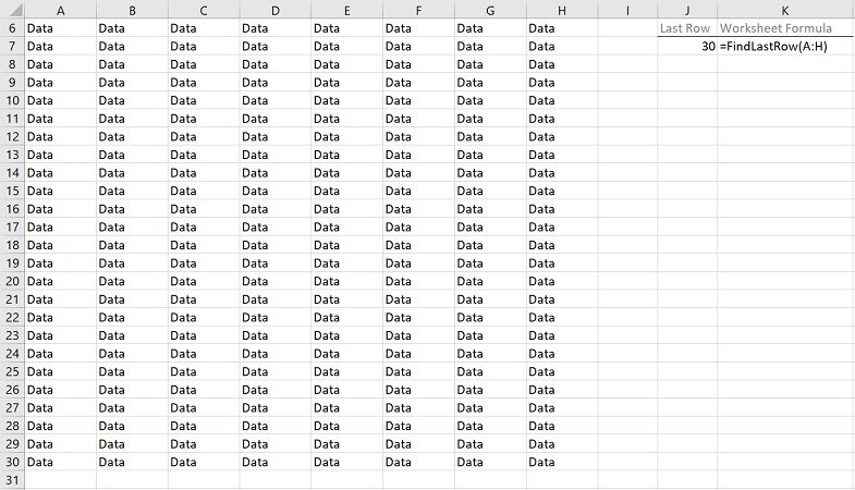
#14. Excel VBA Find Last Column with Data in Cell Range
VBA Code to Find Last Column with Data in Cell Range
To find the last column with data in a cell range, use the following structure/template in the applicable procedure:
If Application.CountA(SearchedCellRangeObject) = 0 Then
    LastColumnVariable = ValueIfCellRangeEmpty
Else
    LastColumnVariable = SearchedCellRangeObject.Find(What:="*", LookIn:=xlFormulas, LookAt:=xlPart, SearchOrder:=xlByColumns, SearchDirection:=xlPrevious).Column
End If
The following Sections describe the main elements in this structure.
Lines #1, #3 and #5: If Application.CountA(SearchedCellRangeObject) = 0 Then | Else | End If
If… Then … Else… End If
The If… Then… Else statement:
- Conditionally executes a set of statements (line #2 or line #4);
- Depending on an expression’s value (Application.CountA(SearchedCellRangeObject) = 0).
Application.CountA(SearchedCellRangeObject) = 0
The condition of an If… Then… Else statement is an expression evaluating to True or False.
- If the expression returns True, a set of statements (line #2) is executed.
- If the expression returns False, a different set of statements (line #4) is executed.
In this expression:
- Application.CountA(…): The WorksheetFunction.CountA method counts the number of cells in a cell range (SearchedCellRangeObject) that are not empty.
- SearchedCellRangeObject: A Range object representing the cell range whose last column you search.
- =: The equal to comparison operator returns True or False as follows:
- True if both expressions (Application.CountA(SearchedCellRangeObject) and 0) are equal.
- False if the expressions (Application.CountA(SearchedCellRangeObject) and 0) are not equal.
- 0: The number 0. The WorksheetFunction.CountA method returns 0 if all cells in SearchedCellRangeObject are empty.
Line #2: LastColumnVariable = ValueIfCellRangeEmpty
Assignment statement assigning:
- ValueIfCellRangeEmpty; to
- LastColumnVariable.
In this expression:
- LastColumnVariable: Variable of (usually) the Long data type holding/representing the number of the last column with data in the cell range whose last column you search (SearchedCellRangeObject).
- =: Assignment operator. Assigns a value (ValueIfCellRangeEmpty) to a variable (LastColumnVariable).
- ValueIfCellRangeEmpty: Value assigned to LastColumnVariable when SearchedCellRangeObject is empty and the WorksheetFunction.CountA method returns 0.
Line #4: LastColumnVariable = SearchedCellRangeObject.Find(What:=”*”, LookIn:=xlFormulas, LookAt:=xlPart, SearchOrder:=xlByColumns, SearchDirection:=xlPrevious).Column
LastColumnVariable
Variable of (usually) the Long data type holding/representing the number of the last column with data in the cell range whose last column you search (SearchedCellRangeObject).
=
The assignment operator assigns a value (SearchedCellRangeObject.Find(What:=”*”, LookIn:=xlFormulas, LookAt:=xlPart, SearchOrder:=xlByColumns, SearchDirection:=xlPrevious).Column) to a variable (LastColumnVariable).
SearchedCellRangeObject
A Range object representing the cell range whose last column you search.
Find
The Range.Find method:
- Finds specific information in a cell range (SearchedCellRangeObject).
- Returns a Range object representing the first cell where the information is found.
What:=”*”
The What parameter of the Range.Find method specifies the data to search for.
To find the last column with data in a cell range, set the What parameter to any character sequence. The asterisk (*) acts as a wildcard and results in Range.Find searching for any character sequence.
LookIn:=xlFormulas
The LookIn parameter of the Range.Find method:
- Specifies the type of data to search in.
- Can take any of the built-in constants/values from the XlFindLookIn enumeration.
To find the last column with data in a cell range, set the LookIn parameter to xlFormulas. xlFormulas refers to formulas.
LookAt:=xlPart
The LookAt parameter of the Range.Find method:
- Specifies against which of the following the data you are searching for is matched:
- The entire/whole searched cell contents.
- Any part of the searched cell contents.
- Can take any of the built-in constants/values from the XlLookAt enumeration.
To find the last column with data in a cell range, set the LookAt parameter to xlPart. xlPart matches the data you are searching for (any character sequence as specified by the What parameter) against any part of the searched cell contents.
SearchOrder:=xlByColumns
The SearchOrder parameter of the Range.Find method:
- Specifies the order in which the applicable cell range (SearchedCellRangeObject) is searched:
- By rows.
- By columns.
- Can take any of the built-in constants/values from the XlSearchOrder enumeration.
To find the last column with data in a cell range, set the SearchOrder parameter to xlByColumns. xlByColumns results in the Range.Find method searching by columns.
SearchDirection:=xlPrevious
The SearchDirection parameter of the Range.Find method:
- Specifies the search direction:
- Search for the previous match.
- Search for the next match.
- Can take any of the built-in constants/values from the XlSearchDirection enumeration.
To find the last column with data in a cell range, set the SearchDirection parameter to xlPrevious. xlPrevious results in the Range.Find method searching for the previous match.
Column
The Range.Column property returns the number of the first column of the first area in a cell range.
When searching for the last column with data in a cell range, the Range.Column property returns the column number of the cell represented by the Range object returned by the Range.Find method (Find(What:=”*”, LookIn:=xlFormulas, LookAt:=xlPart, SearchOrder:=xlByColumns, SearchDirection:=xlPrevious)).
Macro Example to Find Last Column with Data in Cell Range
The following macro (User-Defined Function) example does the following:
- Accepts one argument (MyWorksheetName). This is the name of the worksheet whose last column you search.
- Tests whether the worksheet named MyWorksheetName is empty and proceeds accordingly:
- If the worksheet named MyWorksheetName is empty, returns the number 0 as the number of the last column with data in the worksheet.
- If the worksheet named MyWorksheetName isn’t empty:
- Finds the last column with data in the worksheet; and
- Returns the number of the last column with data in the worksheet.
Function FindLastColumn(MyWorksheetName As String) As Long
    'Source: https://powerspreadsheets.com/
    'For further information: https://powerspreadsheets.com/excel-vba-find/

    'This UDF:
        '(1) Accepts 1 argument: MyWorksheetName
        '(2) Tests whether the worksheet named MyWorksheetName is empty
        '(3) If the worksheet named MyWorksheetName is empty, returns 0 as the number of the last column with data in the worksheet
        '(4) If the worksheet named MyWorksheetName is not empty:
            '(1) Finds the last column with data in the worksheet by searching for the last cell with any character sequence
            '(2) Returns the number of the last column with data in the worksheet

    'Declare object variable to hold/represent all cells in the worksheet named MyWorksheetName
    Dim MyRange As Range

    'Identify all cells in the worksheet named MyWorksheetName
    Set MyRange = ThisWorkbook.Worksheets(MyWorksheetName).Cells

    'Test if MyRange is empty
    If Application.CountA(MyRange) = 0 Then

        'If MyRange is empty, assign 0 to FindLastColumn
        FindLastColumn = 0

    Else

        'If MyRange isn't empty, find the last cell with any character sequence by:
            '(1) Searching for the previous match;
            '(2) Across columns
        FindLastColumn = MyRange.Find(What:="*", LookIn:=xlFormulas, LookAt:=xlPart, SearchOrder:=xlByColumns, SearchDirection:=xlPrevious).Column

    End If

End Function
Effects of Executing Macro Example to Find Last Column with Data in Cell Range
The following image illustrates the effects of using the macro (User-Defined Function) example. In this example:
- Columns A through H (cells A6 to H30) in the worksheet named “Find Last Column Data” contain data.
- Columns A through H of the “Find Last Column Data” worksheet contain exactly the same data as that in the “Find Last Column Formula” worksheet (displayed in the image below).
- The “Find Last Column Data” worksheet contains no data in columns J or K whereas the “Find Last Column Formula” worksheet (displayed in the image below) does.
- Cell J7 contains the worksheet formula that works with the macro (User-Defined Function) example. This worksheet formula returns the number of the last column with data in the worksheet (named “Find Last Column Data”). This is column H or 8.
- Cell K7 displays the worksheet formula used in cell J7 (=FindLastColumn(“Find Last Column Data”)). The name of the worksheet whose last column is searched is “Find Last Column Data”.
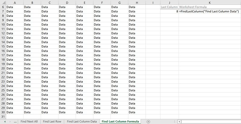
#15. Excel VBA Find Last Non Empty Cell in Column
VBA Code to Find Last Non Empty Cell in Column
To find the last non empty cell in a column, use the following structure/template in the applicable statement:
WorksheetObject.Range(ColumnLetter & WorksheetObject.Rows.Count).End(xlUp)
The following Sections describe the main elements in this structure.
WorksheetObject
A Worksheet object representing the worksheet containing the column whose last non empty cell you want to find.
Range
The Worksheet.Range property returns a Range object representing a cell or cell range.
ColumnLetter
The letter of the column whose last non empty cell you want to find.
&
The concatenation operator joins two strings and creates a new string.
WorksheetObject
A Worksheet object representing the worksheet containing the column whose last non empty cell you want to find.
Rows
The Worksheet.Rows property returns a Range object representing all rows in the applicable worksheet (containing the column whose last non empty cell you want to find).
Count
The Range.Count property returns the number of objects in a collection (the number of rows in the worksheet containing the column whose last non empty cell you want to find).
End(xlUp)
The Range.End property returns a Range object representing the cell at the end of the region containing the source range. In other words: The Range.End property is the rough equivalent of using the “Ctrl + Arrow Key” or “End, Arrow Key” keyboard shortcuts.
The Range.End property accepts one parameter: Direction. Direction:
- Specifies the direction in which to move.
- Can take the any of the built-in constants/values from the XlDirection enumeration.
To find the last non empty cell in a column, set the Direction parameter to xlUp. xlUp:
- Results in moving up, to the top of the data region.
- Is the rough equivalent of the “Ctrl + Up Arrow” or “End, Up Arrow” keyboard shortcuts.
Macro Example to Find Last Non Empty Cell in Column
The following macro (User-Defined Function) example does the following:
- Accepts one argument (MyColumn): The letter of the column (in the worksheet where the UDF is used) whose last non empty cell you want to find.
- Finds the last non empty cell in the applicable column.
- Returns a string containing the address (as an A1-style relative reference) of the last non empty cell in the applicable column.
Function FindLastNonEmptyCellColumn(MyColumn As String) As String
    'Source: https://powerspreadsheets.com/
    'For further information: https://powerspreadsheets.com/excel-vba-find/

    'This UDF:
        '(1) Accepts 1 argument: MyColumn
        '(2) Finds the last non empty cell in the column whose letter is passed as argument (MyColumn) in the worksheet where the UDF is used
        '(3) Returns the address (as an A1-style relative reference) of the last non empty cell found in the column whose letter is passed as argument (MyColumn) in the worksheet where the UDF is used
    With Application.Caller.Parent
        FindLastNonEmptyCellColumn = .Range(MyColumn & .Rows.Count).End(xlUp).Address(RowAbsolute:=False, ColumnAbsolute:=False)
    End With

End Function
Effects of Executing Macro Example to Find Last Non Empty Cell in Column
The following image illustrates the effects of using the macro (User-Defined Function) example. In this example:
- Column A (cells A6 to A30) contains data.
- Cell C7 contains the letter of the column whose last non empty cell is sought (A).
- Cell D7 contains the worksheet formula that works with the macro (User-Defined Function) example. This worksheet formula returns the address (as an A1-style relative reference) of the last non empty cell in column A (MyColumn). This is cell A30
- Cell E7 displays the worksheet formula used in cell D7 (=FindLastNonEmptyCellColumn(C7)). The letter of the column whose last non empty cell is sought is stored in cell C7 (C7).
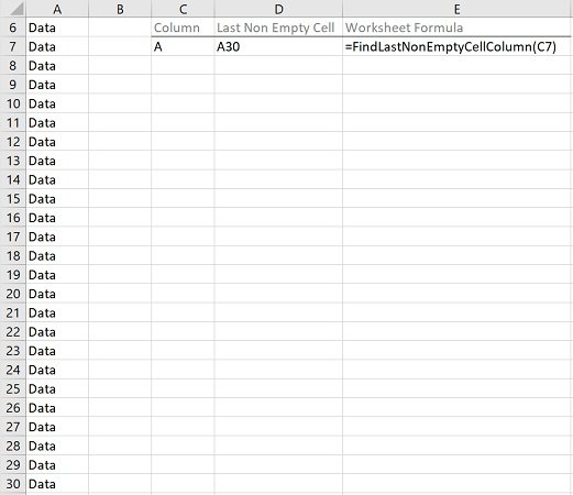
#16. Excel VBA Find Empty (or Blank) Cells
VBA Code to Find Empty (or Blank) Cells
To find all empty (or blank) cells in a cell range, use the following structure/template in the applicable procedure:
Dim BlankCellsObjectVariable As Range
On Error Resume Next
Set BlankCellsObjectVariable = RangeObjectWithBlankCells.SpecialCells(xlCellTypeBlanks)
On Error GoTo 0
If Not BlankCellsObjectVariable Is Nothing Then
    StatementsIfBlankCells
End If
The following Sections describe the main elements in this structure.
Line #1: Dim BlankCellsObjectVariable As Range
Dim
The Dim statement:
- Declares variables.
- Allocates storage space.
BlankCellsObjectVariable
The name of the variable declared with the Dim statement.
BlankCellsObjectVariable holds/represents the empty (or blank) cells found.
As Range
The data type of the variable declared with the Dim statement.
BlankCellsObjectVariable is declared as of the Range object data type. The Range object represents a cell or cell range.
Line #2: On Error Resume Next
The On Error Resume Next statement specifies that, when a run-time error occurs, control passes to the statement immediately following that statement where the error occurred. Therefore, procedure execution continues.
Line #3 returns an error (Run time error ‘1004′: No cells were found) if the cell range where you search for empty (or blank) cells doesn’t contain any empty (or blank) cells.
Line #3: Set BlankCellsObjectVariable = RangeObjectWithBlankCells.SpecialCells(xlCellTypeBlanks)
Set
The Set statement assigns an object reference to an object variable.
BlankCellsObjectVariable
Object variable holding/representing the empty (or blank) cells found.
=
The assignment operator assigns an object reference (returned by the Range.SpecialCells method) to an object variable (BlankCellsObjectVariable).
RangeObjectWithBlankCells
A Range object representing the cell range you search in for empty (or blank) cells.
SpecialCells
The Range.SpecialCells method returns a Range object representing all cells matching a specified:
- Type; and
- Value.
xlCellTypeBlanks
The Type parameter of the Range.SpecialCells method:
- Specifies the cells to include in the Range object returned by the Range.SpecialCells method.
- Can take any of the built-in constants/values from the XlCellType enumeration.
To find all empty (or blank) cells in a cell range, set the Type parameter to xlCellTypeBlanks. xlCellTypeBlanks results in the Range.SpecialCells method including blank/empty cells in the Range object it returns.
Line #4: On Error GoTo 0
The On Error GoTo 0 statement disables error handling (originally enabled by line #2).
Line #5 and #7: If Not BlankCellsObjectVariable Is Nothing Then | End If
If… Then | End If
The If… Then… Else statement:
- Conditionally executes a set of statements (line #6);
- Depending on an expression’s value (Not BlankCellsObjectVariable Is Nothing).
Not BlankCellsObjectVariable Is Nothing
The condition of an If… Then… Else statement is an expression evaluating to True or False. If the expression returns True, the applicable set of statements (line #6) is executed.
In this expression:
- Not BlankCellsObjectVariable:
- The Not operator performs a logical negation on an expression.
- BlankCellsObjectVariable is the object variable holding/representing the empty (or blank) cells found.
- BlankCellsObjectVariable holds/represents Nothing if no empty (or blank) cells are found. Therefore:
- If the Range.SpecialCells method finds no empty (or blank) cells:
- BlankCellsObjectVariable is Nothing.
- Not BlankCellsObjectVariable is not Nothing.
- If the Range.SpecialCells method finds empty (or blank) cells:
- BlankCellsObjectVariable is not Nothing.
- Not BlankCellsObjectVariable is Nothing.
- If the Range.SpecialCells method finds no empty (or blank) cells:
- Is: The Is operator is an object reference comparison operator.
- Nothing: Nothing allows you to disassociate a variable from the data it previously represented. BlankCellsObjectVariable holds/represents Nothing if no empty (or blank) cells are found.
Line #6: StatementsIfBlankCells
Statements conditionally executed by the If… Then… Else statement if the applicable condition (Not BlankCellsObjectVariable Is Nothing) returns True (the Range.SpecialCells method finds empty or blank cells).
Macro Example to Find Empty (or Blank) Cells
The following macro example does the following:
- Find all empty (or blank) cells in the cell range containing cells A6 to H30 in the “Find Blank Cells” worksheet in the workbook where the procedure is stored.
- Set the interior/fill color of all found empty (or blank) cells to light green.
Sub FindBlankCells()
    'Source: https://powerspreadsheets.com/
    'For further information: https://powerspreadsheets.com/excel-vba-find/

    'This procedure:
        '(1) Finds all blank cells in cells A6 to H30 of the "Find Blank Cells" worksheet in this workbook
        '(2) Sets the found cells' interior/fill color to light green

    'Declare object variable to hold/represent blank cells
    Dim MyBlankCells As Range

    'Enable error-handling
    On Error Resume Next

    'Identify blank cells in searched cell range
    Set MyBlankCells = ThisWorkbook.Worksheets("Find Blank Cells").Range("A6:H30").SpecialCells(xlCellTypeBlanks)

    'Disable error-handling
    On Error GoTo 0

    'Test whether blank cells were found in searched cell range
    If Not MyBlankCells Is Nothing Then

        'Set interior/fill color of blank cells found to light green
        MyBlankCells.Interior.Color = RGB(63, 189, 133)

    End If

End Sub
Effects of Executing Macro Example to Find Empty (or Blank) Cells
The following image illustrates the effects of using the macro example. In this example:
- Columns A through H (cells A6 to H30) contain:
- Data; and
- A few empty cells (with light green interior/fill).
- A text box (Find all blank cells) executes the macro example when clicked.
After the macro is executed, Excel sets the interior/fill color of all empty (or blank) cells to light green.

#17. Excel VBA Find First Empty (or Blank) Cell in Cell Range
VBA Code to Find First Empty (or Blank) Cell in Cell Range
To find the first empty (or blank) cell in a cell range, use the following structure/template in the applicable procedure:
For Each iCell In CellRangeObject
    If IsEmpty(iCell) Then
        StatementsForFirstEmptyCell
        Exit For
    End If
Next iCell
The following Sections describe the main elements in this structure.
Lines #1 and #6: For Each iCell In CellRangeObject | Next iCell
For Each … In … | Next …
The For Each… Next statement repeats a series of statements for each element (iCell, an individual cell) in a collection (CellRangeObject).
iCell
Object variable (of the Range data type) used to iterate/loop through each element of the collection (CellRangeObject).
CellRangeObject
A Range object representing the cell range you search in.
The series of statements repeated by the For Each… Next statement are repeated for each individual element (iCell) in CellRangeObject.
Lines #2 and #5: If IsEmpty(iCell) Then | End If
If… Then | End If
The If… Then Else statement:
- Conditionally executes a set of statements (lines #3 and #4);
- Depending on an expression’s value (IsEmpty(iCell)).
IsEmpty(iCell)
The condition of an If… Then… Else statement is an expression evaluating to True or False. If the expression returns True, the applicable set of statements (lines #3 and #4) are executed.
In this expression:
- As a general rule, the IsEmpty function returns a Boolean value (True or False) indicating whether a variable is initialized. You can (also) use the IsEmpty function to test whether a cell is empty (or blank).
- iCell is an object variable representing the individual cell the For Each… Next statement is currently working with (iterating through).
- IsEmpty(iCell) returns True or False as follows:
- True if the cell (currently) represented by iCell is empty (or blank).
- False if the cell (currently) represented by iCell isn’t empty. A cell isn’t considered to be empty if, for example, it contains a worksheet formula returning a zero-length string (“”).
Line #3: StatementsForFirstEmptyCell
Statements conditionally executed by the If… Then… Else statement if the applicable condition (IsEmpty(iCell)) returns True (the cell currently represented by iCell is empty or blank).
Line #4: Exit For
The Exit For statement:
- Exits a For Each… Next loop.
- Transfers control to the statement following the Next statement (line #6).
Macro Example to Find First Empty (or Blank) Cell in Cell Range
The following macro (User-Defined Function) example does the following:
- Accepts one argument (MyRange): The cell range whose first empty cell you search for.
- Loops through each individual cell in the cell range (MyRange) and tests whether the applicable cell is empty (or blank).
- Returns the following:
- If MyRange contains empty cells, the address (as an A1-style relative reference) of the first empty cell in the cell range (MyRange).
- If MyRange doesn’t contain empty cells, the string “No empty cells found in cell range”.
Function FindNextEmptyCellRange(MyRange As Range) As String
    'Source: https://powerspreadsheets.com/
    'For further information: https://powerspreadsheets.com/excel-vba-find/

    'This UDF:
        '(1) Accepts 1 argument: MyRange
        '(2) Loops through each individual cell in the cell range (MyRange) and tests whether the applicable cell is empty
        '(3) Returns the following (as applicable):
            'If there are empty cells in MyRange: The address (as an A1-style relative reference) of the first empty cell
            'If there are no empty cells in MyRange: The string "No empty cells found in cell range"

    'Declare object variable to iterate/loop through all cells in the cell range (MyRange)
    Dim iCell As Range

    'Loop through each cell in the cell range (MyRange)
    For Each iCell In MyRange

        'If the current cell is empty:
            '(1) Return the current cell's address (as an A1-style relative reference)
            '(2) Exit the For Each... Next loop
        If IsEmpty(iCell) Then
            FindNextEmptyCellRange = iCell.Address(RowAbsolute:=False, ColumnAbsolute:=False)
            Exit For
        End If

    Next iCell

    'If no empty cells are found in the cell range (MyRange), return the string "No empty cells found in cell range"
    If FindNextEmptyCellRange = "" Then FindNextEmptyCellRange = "No empty cells found in cell range"

End Function
Effects of Executing Macro Example to Find First Empty (or Blank) Cell in Cell Range
The following image illustrates the effects of using the macro (User-Defined Function) example. In this example:
- Columns A through H (cells A6 to H30) contain:
- Data; and
- A few empty cells (with light green interior/fill).
- Cell J7 contains the worksheet formula that works with the macro (User-Defined Function) example. This worksheet formula returns the address (as an A1-style relative reference) of the first empty cell in the cell range (MyRange). This is cell B7.
- Cell K7 displays the worksheet formula used in cell J7 (=FindNextEmptyCellRange(A6:H30)). The cell range where the search is carried out contains cells A6 to H30 (A6:H30).
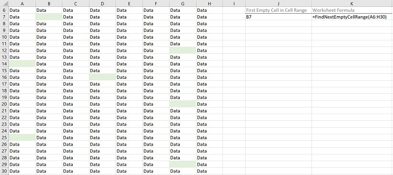
#18. Excel VBA Find First Empty (or Blank) Cell in Column
VBA Code to Find First Empty (or Blank) Cell in Column
To find the first empty (or blank) cell in a column, use the following structure/template in the applicable statement:
ColumnRangeObject.Find(What:="", After:=ColumnRangeObject.Cells(ColumnRangeObject.Cells.Count), LookIn:=xlFormulas, LookAt:=xlWhole, SearchOrder:=xlByRows, SearchDirection:=xlNext)
The following Sections describe the main elements in this structure.
ColumnRangeObject
A Range object representing the column whose first empty (or blank) cell you search for.
Find
The Range.Find method:
- Finds specific information (the first empty or blank cell) in a cell range (ColumnRangeObject).
- Returns a Range object representing the first cell where the information is found.
What:=””
The What parameter of the Range.Find method specifies the data to search for.
To find the first empty (or blank) cell in a column, set the What parameter to a zero-length string (“”).
After:=ColumnRangeObject.Cells(ColumnRangeObject.Cells.Count)
The After parameter of the Range.Find method specifies the cell after which the search begins.
To find the first empty (or blank) cell in a column, set the After parameter to “ColumnRangeObject.Cells(ColumnRangeObject.Cells.Count)”. For these purposes:
- “ColumnRangeObject” is a Range object representing the column whose first empty (or blank) cell you search for.
- The Range.Cells property (Cells) returns a Range object representing all cells in the column whose first empty (or blank) cell you search for.
- The Range.Item property returns a Range object representing the last cell in the column whose first empty (or blank) cell you search for. For these purposes, the RowIndex parameter of the Range.Item property is set to the value returned by the Range.Count property (Count).
- The Range.Count property (Count) returns the number of cells in the Range object returned by the Range.Cells property (ColumnRangeObject.Cells).
LookIn:=xlFormulas
The LookIn parameter of the Range.Find method:
- Specifies the type of data to search in.
- Can take any of the built-in constants/values from the XlFindLookIn enumeration.
To find the first empty (or blank) cell in a column, set the LookIn parameter to xlFormulas. xlFormulas refers to formulas.
LookAt:=xlWhole
The LookAt parameter of the Range.Find method:
- Specifies against which of the following the data you are searching for is matched:
- The entire/whole searched cell contents.
- Any part of the searched cell contents.
- The LookAt parameter can take any of the built-in constants/values from the XlLookAt enumeration.
To find the first empty (or blank) cell in a column, set the LookAt parameter to xlWhole. xlWhole matches the data you are searching for against the entire/whole searched cell contents.
SearchOrder:=xlByRows
The SearchOrder parameter of the Range.Find method:
- Specifies the order in which the applicable cell range (ColumnRangeObject) is searched:
- By rows.
- By columns.
- Can take any of the built-in constants/values from the XlSearchOrder enumeration.
To find the first empty (or blank) cell in a column, set the SearchOrder parameter to xlByRows. xlByRows searches by rows.
SearchDirection:=xlNext
The SearchDirection parameter of the Range.Find method:
- Specifies the search direction:
- Search for the previous match.
- Search for the next match.
- Can take any of the built-in constants/values from the XlSearchDirection enumeration.
To find the first empty (or blank) cell in a column, set the SearchDirection parameter to xlNext. xlNext searches for the next match.
Macro Example to Find First Empty (or Blank) Cell in Column
The following macro (User-Defined Function) example does the following:
- Accepts one argument (MyColumn): The letter of the column (in the worksheet where the UDF is used) whose first empty (or blank) cell you search for.
- Finds the first empty (or blank) cell in the applicable column.
- Returns a string containing the address (as an A1-style relative reference) of the first empty (or blank) cell in the applicable column.
Function FindFirstEmptyCellColumn(MyColumn As String) As String
    'Source: https://powerspreadsheets.com/
    'For further information: https://powerspreadsheets.com/excel-vba-find/

    'This UDF:
        '(1) Accepts 1 argument: MyColumn
        '(2) Finds the first empty (blank) cell in the column whose letter is passed as argument (MyColumn) in the worksheet where the UDF is used
        '(3) Returns the address (as an A1-style relative reference) of the first empty (blank) cell in the column whose letter is passed as argument (MyColumn) in the worksheet where the UDF is used
    With Application.Caller.Parent.Columns(MyColumn)
        FindFirstEmptyCellColumn = .Find(What:="", After:=.Cells(.Cells.Count), LookIn:=xlFormulas, LookAt:=xlWhole, SearchOrder:=xlByRows, SearchDirection:=xlNext).Address(RowAbsolute:=False, ColumnAbsolute:=False)
    End With

End Function
Effects of Executing Macro Example to Find First Empty (or Blank) Cell in Column
The following image illustrates the effects of using the macro (User-Defined Function) example. In this example:
- Column I (cells I1 to I25) contains:
- Data; and
- A few empty cells (with light green interior/fill).
- Cell A7 contains the letter of the column whose first empty (or blank) cell is sought (I).
- Cell B7 contains the worksheet formula that works with the macro (User-Defined Function) example. This worksheet formula returns the address (as an A1-style relative reference) of the first empty (or blank) cell in column I (MyColumn). This is cell I10.
- Cell C7 displays the worksheet formula used in cell B7 (=FindFirstEmptyCellColumn(A7)). The letter of the column whose first empty (or blank) cell is sought is stored in cell A7 (A7).

#19. Excel VBA Find Next Empty (or Blank) Cell in Column
VBA Code to Find Next Empty (or Blank) Cell in Column
To find the next empty (or blank) cell in a column, use the following structure/template in the applicable procedure:
If IsEmpty(RangeObjectSourceCell) Then
    RangeObjectSourceCell.ActionForNextEmptyCell
ElseIf IsEmpty(RangeObjectSourceCell.Offset(1, 0)) Then
    RangeObjectSourceCell.Offset(1, 0).ActionForNextEmptyCell
Else
    RangeObjectSourceCell.End(xlDown).Offset(1, 0).ActionForNextEmptyCell
End If
The following Sections describe the main elements in this structure.
Lines #1, #3, #5 and #7: If IsEmpty(RangeObjectSourceCell) Then | ElseIf IsEmpty(RangeObjectSourceCell.Offset(1, 0)) Then | Else | End If
If… Then | ElseIf… Then | Else | End If
The If… Then… Else statement:
- Conditionally executes a set of statements (lines #2, #4 or #6);
- Depending on an expression’s value (IsEmpty(RangeObjectSourceCell) or IsEmpty(RangeObjectSourceCell.Offset(1, 0))).
IsEmpty(RangeObjectSourceCell)
The condition of an If… Then… Else statement is an expression evaluating to True or False. If the expression returns True, the applicable set of statements (line #2) is executed.
In this expression:
- As a general rule, the IsEmpty function returns a Boolean value (True or False) indicating whether a variable is initialized. You can (also) use the IsEmpty function to test whether a cell is empty (or blank).
- RangeObjectSourceCell is a Range object representing the cell where the search (for the next empty or blank cell in the column) begins.
- IsEmpty(RangeObjectSourceCell) returns True or False as follows:
- True if the cell represented by RangeObjectSourceCell is empty (or blank).
- False if the cell represented by RangeObjectSourceCell isn’t empty. A cell isn’t considered to be empty if, for example, it contains a worksheet formula returning a zero-length string (“”).
IsEmpty(RangeObjectSourceCell.Offset(1, 0))
The condition of an If… Then… Else statement is an expression evaluating to True or False. If the expression returns True, the applicable set of statements (line #4) is executed.
In this expression:
- As a general rule, the IsEmpty function returns a Boolean value (True or False) indicating whether a variable is initialized. You can (also) use the IsEmpty function to test whether a cell is empty (or blank).
- RangeObjectSourceCell is a Range object representing the cell where the search (for the next empty or blank cell in the column) begins.
- The Range.Offset property (Offset(1, 0)) returns a Range object representing a cell range at an offset from the source cell range. In this expression:
- The source cell range is the cell where the search (for the next empty or blank cell in the column) begins (RangeObjectSourceCell).
- The offset from the source cell range is as follows:
- 1 row downwards, as specified by the RowOffset parameter of the Range.Offset property (1).
- No column offsetting, as specified by the ColumnOffset parameter of the Range.Offset property (0).
- IsEmpty(RangeObjectSourceCell.Offset(1, 0)) returns True or False as follows:
- True if the cell represented by the Range object returned by the Range.Offset property is empty.
- False if the cell represented by the Range object returned by the Range.Offset property isn’t empty. A cell isn’t considered to be empty if, for example, it contains a worksheet formula returning a zero-length string (“”).
Line #2: RangeObjectSourceCell.ActionForNextEmptyCell
Statement conditionally executed by the If… Then… Else statement if the applicable condition (IsEmpty(RangeObjectSourceCell)) returns True.
RangeObjectSourceCell
A Range object representing the cell where the search (for the next empty or blank cell in the column) begins.
ActionForNextEmptyCell
VBA construct (usually a property or method) working with the applicable cell (represented by RangeObjectSourceCell).
Line #4: RangeObjectSourceCell.Offset(1, 0).ActionForNextEmptyCell
Statement conditionally executed by the If… Then… Else statement if the applicable condition (IsEmpty(RangeObjectSourceCell.Offset(1, 0))) returns True.
RangeObjectSourceCell
A Range object representing the cell where the search (for the next empty or blank cell in the column) begins.
Offset(1, 0)
The Range.Offset property (Offset(1, 0)) returns a Range object representing a cell range at an offset from the source cell range. For these purposes:
- The source cell range is the cell where the search (for the next empty or blank cell in the column) begins (RangeObjectSourceCell).
- The offset from the source cell range is as follows:
- 1 row downwards, as specified by the RowOffset parameter of the Range.Offset property (1).
- No column offsetting, as specified by the ColumnOffset parameter of the Range.Offset property (0).
ActionForNextEmptyCell
VBA construct (usually a property or method) working with the applicable cell (returned by the Range.Offset property).
Line #6: RangeObjectSourceCell.End(xlDown).Offset(1, 0).ActionForNextEmptyCell
Statement conditionally executed by the If… Then… Else statement if no previous condition (in lines #1 or #3) returns True.
RangeObjectSourceCell
A Range object representing the cell where the search (for the next empty or blank cell in the column) begins.
End(xlDown)
The Range.End property returns a Range object representing the cell at the end of the region containing the source range. In other words: The Range.End property is the rough equivalent of using the “Ctrl + Arrow Key” or “End, Arrow Key” keyboard shortcuts.
The Range.End property accepts one parameter: Direction. Direction:
- Specifies the direction in which to move.
- Can take the any of the built-in constants/values from the XlDirection enumeration.
To find the next empty (or blank) cell in a column, set the Direction parameter to xlDown. xlDown:
- Results in moving down, to the bottom of the data region.
- Is the rough equivalent of the “Ctrl + Down Arrow” or “End, Down Arrow” keyboard shortcuts.
Offset(1, 0)
The Range.Offset property (Offset(1, 0)) returns a Range object representing a cell range at an offset from the source cell range. For these purposes:
- The source cell range is the cell represented by the Range object returned by the Range.End property (End(xlDown)).
- The offset from the source cell range is as follows:
- 1 row downwards, as specified by the RowOffset parameter of the Range.Offset property (1).
- No column offsetting, as specified by the ColumnOffset parameter of the Range.Offset property (0).
ActionForNextEmptyCell
VBA construct (usually a property or method) working with the applicable cell (returned by the Range.Offset property).
Macro Example to Find Next Empty (or Blank) Cell in Column
The following macro (User-Defined Function) example does the following:
- Accepts one argument (MySourceCell): The cell where the search (for the next empty or blank cell in the column) begins.
- Finds the next empty (or blank) cell in the applicable column after MySourceCell.
- Returns a string containing the address (as an R1C1-style absolute reference) of the next empty (or blank) cell in the applicable column.
Function FindNextEmptyCellColumn(MySourceCell As Range) As String
    'Source: https://powerspreadsheets.com/
    'For further information: https://powerspreadsheets.com/excel-vba-find/

    'This UDF:
        '(1) Accepts 1 argument: MySourceCell
        '(2) Finds the next empty/blank cell in the applicable column and after the cell passed as argument (MySourceCell)
        '(3) Returns the address (as an R1C1-style absolute reference) of the next empty/blank cell in the applicable column and after the cell passed as argument (MySourceCell)

    With MySourceCell(1)

        'If first cell in cell range passed as argument (MySourceCell) is empty, obtain/return that cell's address
        If IsEmpty(MySourceCell(1)) Then
            FindNextEmptyCellColumn = .Address(ReferenceStyle:=xlR1C1)

        'If cell below first cell in cell range passed as argument (MySourceCell) is empty, obtain/return that cell's address
        ElseIf IsEmpty(.Offset(1, 0)) Then
            FindNextEmptyCellColumn = .Offset(1, 0).Address(ReferenceStyle:=xlR1C1)

        'Otherwise:
            '(1) Find the next empty/blank cell in the applicable column and after the first cell in cell range passed as argument (MySourceCell)
            '(2) Obtain/return the applicable cell's address
        Else
            FindNextEmptyCellColumn = .End(xlDown).Offset(1, 0).Address(ReferenceStyle:=xlR1C1)
        End If

    End With

End Function
Effects of Executing Macro Example to Find Next Empty (or Blank) Cell in Column
The following image illustrates the effects of using the macro (User-Defined Function) example. In this example:
- Column A (cells A6 to A30) contains:
- Data; and
- A few empty cells.
- Cell C7 contains the worksheet formula that works with the macro (User-Defined Function) example. This worksheet formula returns the address (as an R1C1-style absolute reference) of the next empty (or blank) cell in column A after cell A13 (MySourceCell). This cell R21C1 (or A21 as an A1-style relative reference).
- Cell D7 displays the worksheet formula used in cell C7 (=FindNextEmptyCellColumn(A13)). The cell where the search (for the next empty or blank cell in the column) begins is A13 (A13).
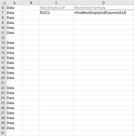
#20. Excel VBA Find Value in Array
VBA Code to Find Value in Array
To find a numeric value in a one-dimensional array, use the following structure/template in the applicable procedure:
Dim PositionOfValueInArray As Variant
Dim LoopCounter As Long
PositionOfValueInArray = OutputIfValueNotInArray
For LoopCounter = LBound(SearchedArray) To UBound(SearchedArray)
    If SearchedArray(LoopCounter) = SearchedValue Then
        PositionOfValueInArray = LoopCounter
        Exit For
    End If
Next LoopCounter
The following Sections describe the main elements in this structure.
Lines #1 and #2: Dim PositionOfValueInArray As Variant | Dim LoopCounter As Long
The Dim statement:
- Declares variables.
- Allocates storage space.
PositionOfValueInArray | LoopCounter
The names of the variables declared with the Dim statement.
- PositionOfValueInArray holds/represents:
- The position of the searched numeric value in the array, if the searched numeric value is found in the array.
- The default/fallback output/data, if the searched numeric value isn’t found in the array.
- LoopCounter represents the loop counter used in the For… Next loop in lines #4 to #9.
As Variant | As Long
The data type of the variables declared with the Dim statement.
- PositionOfValueInArray is of the Variant data type. The Variant data type can (generally) contain any type of data, except for fixed-length Strings.
- LoopCounter is of the Long data type. The Long data type can contain integers between -2,147,483,648 and 2,147,483,647.
Line #3: PositionOfValueInArray = OutputIfValueNotInArray
PositionOfValueInArray
Variable holding/representing:
- The position of the searched numeric value in the array, if the searched numeric value is found in the array.
- The default/fallback output/data, if the searched numeric value isn’t found in the array.
=
The assignment operator assigns the result returned by an expression (OutputIfValueNotInArray) to a variable (PositionOfValueInArray).
OutputIfValueNotInArray
Expression specifying the default/fallback output/data to be assigned to the PositionOfValueInArray variable if the searched numeric value isn’t found in the array.
Lines #4 and #9: For LoopCounter = LBound(SearchedArray) To UBound(SearchedArray) | Next LoopCounter
For… = … To … | Next…
The For… Next statement repeats a series of statements a specific number of times.
LoopCounter
Variable holding/representing the loop counter.
LBound(…) | UBound(…)
The LBound/UBound functions return the lower/upper bound of an array’s dimension. The LBound/UBound functions accept two arguments:
- ArrayName: The name of the array whose lower/upper bound you want to obtain.
- Dimension:
- An optional argument.
- The dimension (of the applicable array) whose lower/upper bound you want to obtain.
If you omit specifying the Dimension argument, the LBound/UBound functions return the lower/upper bound of the array’s first dimension.
The initial/final values of LoopCounter are set to the following:
- Initial value (Start) of LoopCounter: The output returned by the LBound function (LBound(SearchedArray)).
- Final value (End) of LoopCounter: The output returned by the UBound function (UBound(SearchedArray)).
SearchedArray
The array you search in.
SearchedArray is passed as the ArrayName argument of the LBound/UBound functions.
Lines #5 and #8: If SearchedArray(LoopCounter) = SearchedValue Then | End If
If… Then… End If
The If… Then… Else statement:
- Conditionally executes a set of statements (lines #6 and #7);
- Depending on an expression’s value (SearchedArray(LoopCounter) = SearchedValue).
SearchedArray(LoopCounter) = SearchedValue
The condition of an If… Then… Else statement is an expression evaluating to True or False.
- If the expression returns True, a set of statements (lines #6 and #7) is executed.
- If the expression returns False:
- No statements are executed.
- Execution continues with the statement following End If (line #8).
In this expression:
- SearchedArray: The array you search in.
- LoopCounter: Variable holding/representing the loop counter.
- SearchedArray(LoopCounter): Array element whose index number is LoopCounter.
- =: The equal to comparison operator returns True or False as follows:
- True if both expressions (SearchedArray(LoopCounter) and SearchedValue) are equal.
- False if the expressions (SearchedArray(LoopCounter) and SearchedValue) are not equal.
- SearchedValue: Numeric value you search for in the array (SearchedArray).
Line #6: PositionOfValueInArray = LoopCounter
PositionOfValueInArray
Variable holding/representing:
- The position of the searched numeric value in the array, if the searched numeric value is found in the array.
- The default/fallback output/data, if the searched numeric value isn’t found in the array.
=
The assignment operator assigns the result returned by an expression (LoopCounter) to a variable (PositionOfValueInArray).
LoopCounter
Variable holding/representing the loop counter.
Line #7: Exit For
The Exit For statement:
- Exits a For… Next loop.
- Transfers control to the statement following the Next statement (line #8).
Macro Example to Find Value in Array
The following macro (User-Defined Function) example does the following:
- Accepts two arguments:
- MyArray: The array you search in.
- MyValue: The numeric value you search for.
- Loops through each element in MyArray and tests whether the applicable element is equal to MyValue.
- Returns the following:
- If MyValue is not found in MyArray, the string “Value not found in array”.
- If MyValue is found in MyArray, the position/index number of MyValue in MyArray.
Function FindValueInArray(MyArray As Variant, MyValue As Variant) As Variant
    'Source: https://powerspreadsheets.com/
    'For further information: https://powerspreadsheets.com/excel-vba-find/

    'This UDF:
        '(1) Accepts 2 arguments: MyArray and MyValue
        '(2) Loops through each element in the array (MyArray) and tests whether the applicable element is equal to the searched value (MyValue)
        '(3) Returns the following (as applicable):
            'If MyValue is not found in MyArray: The string "Value not found in array"
            'If MyValue is found in MyArray: The position (index number) of MyValue in MyArray

    'Declare variable to represent loop counter
    Dim iCounter As Long

    'Specify default/fallback value/string to be returned ("Value not found in array") if MyValue is not found in MyArray
    FindValueInArray = "Value not found in array"

    'Loop through each element in the array (MyArray)
    For iCounter = LBound(MyArray) To UBound(MyArray)

        'Test if the current array element is equal to MyValue
        If MyArray(iCounter) = MyValue Then

            'If the current array element is equal to MyValue:
                '(1) Return the position (index number) of the current array element
                '(2) Exit the For... Next loop
            FindValueInArray = iCounter
            Exit For

        End If

    Next iCounter

End Function
Effects of Executing Macro Example to Find Value in Array
To illustrate the effects of using the macro (User-Defined Function) example, I use the following macro. The following macro does the following:
- Declare an array (MySearchedArray).
- Fill the array with values (0, 10, 20, …, 90).
- Call the FindValueInArray macro (User-Defined Function) example to find the number “50” in the array.
- Display a message box with the value/string returned by the FindValueInArray macro (User-Defined Function) example.
Sub FindValueInArrayCaller()
    'Source: https://powerspreadsheets.com/
    'For further information: https://powerspreadsheets.com/excel-vba-find/

    'This procedure:
        '(1) Declares an array and fills it with values (0, 10, 20, ..., 90)
        '(2) Calls the FindValueInArray UDF to find the number "50" in the array
        '(3) Displays a message box with the value/string returned by the FindValueInArray UDF

    'Declare a zero-based array with 10 elements of the Long data type
    Dim MySearchedArray(0 To 9) As Long

    'Assign values to array elements
    MySearchedArray(0) = 0
    MySearchedArray(1) = 10
    MySearchedArray(2) = 20
    MySearchedArray(3) = 30
    MySearchedArray(4) = 40
    MySearchedArray(5) = 50
    MySearchedArray(6) = 60
    MySearchedArray(7) = 70
    MySearchedArray(8) = 80
    MySearchedArray(9) = 90

    'Do the following:
        '(1) Call the FindValueInArray UDF and search for the number "50" in MySearchedArray
        '(2) Display a message box with the value/string returned by the FindValueInArray UDF
    MsgBox FindValueInArray(MySearchedArray, 50)


End Sub
The following GIF illustrates the effects of using the macro above to call the macro (User-Defined Function) example.
As expected, this results in Excel displaying a message box with the number 5. This is the position of the searched numeric value (50) in the array.

Learn More About Excel VBA Find
Workbook Example Used in this Excel VBA Find Tutorial
This VBA Find Tutorial is accompanied by an Excel workbook containing the data and macros I use in the examples above. You can get free access to this example workbook by clicking the button below.
The Power Spreadsheets Library
The Books at The Power Spreadsheets Library are comprehensive and actionable guides for professionals who want to:
- Automate Excel;
- Save time for the things that really matter; and
- Open new career opportunities.
Learn more about The Power Spreadsheets Library here.