
MATCH function
Tip: Try using the new XMATCH function, an improved version of MATCH that works in any direction and returns exact matches by default, making it easier and more convenient to use than its predecessor.
The MATCH function searches for a specified item in a range of cells, and then returns the relative position of that item in the range. For example, if the range A1:A3 contains the values 5, 25, and 38, then the formula =MATCH(25,A1:A3,0) returns the number 2, because 25 is the second item in the range.

Tip: Use MATCH instead of one of the LOOKUP functions when you need the position of an item in a range instead of the item itself. For example, you might use the MATCH function to provide a value for the row_num argument of the INDEX function.
Syntax
MATCH(lookup_value, lookup_array, [match_type])
The MATCH function syntax has the following arguments:
-
lookup_value Required. The value that you want to match in lookup_array. For example, when you look up someone’s number in a telephone book, you are using the person’s name as the lookup value, but the telephone number is the value you want.
The lookup_value argument can be a value (number, text, or logical value) or a cell reference to a number, text, or logical value.
-
lookup_array Required. The range of cells being searched.
-
match_type Optional. The number -1, 0, or 1. The match_type argument specifies how Excel matches lookup_value with values in lookup_array. The default value for this argument is 1.
The following table describes how the function finds values based on the setting of the match_type argument.
|
Match_type |
Behavior |
|
1 or omitted |
MATCH finds the largest value that is less than or equal to lookup_value. The values in the lookup_array argument must be placed in ascending order, for example: …-2, -1, 0, 1, 2, …, A-Z, FALSE, TRUE. |
|
0 |
MATCH finds the first value that is exactly equal to lookup_value. The values in the lookup_array argument can be in any order. |
|
-1 |
MATCH finds the smallest value that is greater than or equal tolookup_value. The values in the lookup_array argument must be placed in descending order, for example: TRUE, FALSE, Z-A, …2, 1, 0, -1, -2, …, and so on. |
-
MATCH returns the position of the matched value within lookup_array, not the value itself. For example, MATCH(«b»,{«a»,»b»,»c«},0) returns 2, which is the relative position of «b» within the array {«a»,»b»,»c»}.
-
MATCH does not distinguish between uppercase and lowercase letters when matching text values.
-
If MATCH is unsuccessful in finding a match, it returns the #N/A error value.
-
If match_type is 0 and lookup_value is a text string, you can use the wildcard characters — the question mark (?) and asterisk (*) — in the lookup_value argument. A question mark matches any single character; an asterisk matches any sequence of characters. If you want to find an actual question mark or asterisk, type a tilde (~) before the character.
Example
Copy the example data in the following table, and paste it in cell A1 of a new Excel worksheet. For formulas to show results, select them, press F2, and then press Enter. If you need to, you can adjust the column widths to see all the data.
|
Product |
Count |
|
|
Bananas |
25 |
|
|
Oranges |
38 |
|
|
Apples |
40 |
|
|
Pears |
41 |
|
|
Formula |
Description |
Result |
|
=MATCH(39,B2:B5,1) |
Because there is not an exact match, the position of the next lowest value (38) in the range B2:B5 is returned. |
2 |
|
=MATCH(41,B2:B5,0) |
The position of the value 41 in the range B2:B5. |
4 |
|
=MATCH(40,B2:B5,-1) |
Returns an error because the values in the range B2:B5 are not in descending order. |
#N/A |
Need more help?
Содержание
- MATCH
- Syntax
- Example
- How to Find Matching Values in Excel
- What’s An Excel Function?
- The Exact Function
- The MATCH Function
- The VLOOKUP Function
- How Do I Find Matching Values in Two Different Sheets?
- How Else Can I Use These Functions?
- Comparison of two tables in Excel for finding matches in columns
- Comparing two columns for finding matches in Excel
- Principle of comparing the data of two columns in Excel
MATCH
Tip: Try using the new XMATCH function, an improved version of MATCH that works in any direction and returns exact matches by default, making it easier and more convenient to use than its predecessor.
The MATCH function searches for a specified item in a range of cells, and then returns the relative position of that item in the range. For example, if the range A1:A3 contains the values 5, 25, and 38, then the formula =MATCH(25,A1:A3,0) returns the number 2, because 25 is the second item in the range.
Tip: Use MATCH instead of one of the LOOKUP functions when you need the position of an item in a range instead of the item itself. For example, you might use the MATCH function to provide a value for the row_num argument of the INDEX function.
Syntax
MATCH(lookup_value, lookup_array, [match_type])
The MATCH function syntax has the following arguments:
lookup_value Required. The value that you want to match in lookup_array. For example, when you look up someone’s number in a telephone book, you are using the person’s name as the lookup value, but the telephone number is the value you want.
The lookup_value argument can be a value (number, text, or logical value) or a cell reference to a number, text, or logical value.
lookup_array Required. The range of cells being searched.
match_type Optional. The number -1, 0, or 1. The match_type argument specifies how Excel matches lookup_value with values in lookup_array. The default value for this argument is 1.
The following table describes how the function finds values based on the setting of the match_type argument.
MATCH finds the largest value that is less than or equal to lookup_value. The values in the lookup_array argument must be placed in ascending order, for example: . -2, -1, 0, 1, 2, . A-Z, FALSE, TRUE.
MATCH finds the first value that is exactly equal to lookup_value. The values in the lookup_array argument can be in any order.
MATCH finds the smallest value that is greater than or equal to lookup_value. The values in the lookup_array argument must be placed in descending order, for example: TRUE, FALSE, Z-A, . 2, 1, 0, -1, -2, . and so on.
MATCH returns the position of the matched value within lookup_array, not the value itself. For example, MATCH(«b», <«a»,»b»,»c «>,0) returns 2, which is the relative position of «b» within the array <«a»,»b»,»c»>.
MATCH does not distinguish between uppercase and lowercase letters when matching text values.
If MATCH is unsuccessful in finding a match, it returns the #N/A error value.
If match_type is 0 and lookup_value is a text string, you can use the wildcard characters — the question mark ( ?) and asterisk ( *) — in the lookup_value argument. A question mark matches any single character; an asterisk matches any sequence of characters. If you want to find an actual question mark or asterisk, type a tilde (
) before the character.
Example
Copy the example data in the following table, and paste it in cell A1 of a new Excel worksheet. For formulas to show results, select them, press F2, and then press Enter. If you need to, you can adjust the column widths to see all the data.
Источник
How to Find Matching Values in Excel
Ladies and gentlemen, introducing the Exact function
You’ve got an Excel workbook with thousands of numbers and words. There are bound to be multiples of the same number or word in there. You might need to find them. So we’re going to look at several ways you can find matching values in Excel 365.
We’re going to cover finding the same words or numbers in two different worksheets and in two different columns. We’ll look at using the EXACT, MATCH, and VLOOKUP functions. Some of the methods we’ll use may not work in the web version of Microsoft Excel, but they will all work in the desktop version.
What’s An Excel Function?
If you’ve used functions before, skip ahead.
An Excel function is like a mini app. It applies a series of steps to perform a single task. The most commonly used Excel functions can be found in the Formulas tab. Here we see them categorized by the nature of the function –
- AutoSum
- Recently Used
- Financial
- Logical
- Text
- Date & Time
- Lookup & Reference
- Math & Trig
- More Functions.
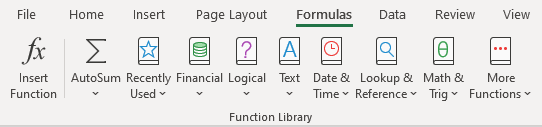
The More Functions category contains the categories Statistical, Engineering, Cube, Information, Compatibility, and Web.
The Exact Function
The Exact function’s task is to go through the rows of two columns and find matching values in the Excel cells. Exact means exact. On its own, the Exact function is case sensitive. It won’t see New York and new york as being a match.
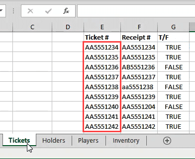
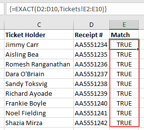
In the example below, there are two columns of text – Tickets and Receipts. For only 10 sets of text, we could compare them by looking at them. Imagine if there were 1,000 rows or more though. That’s when you would use the Exact function.
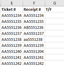
Place the cursor in cell C2. In the formula bar, enter the formula
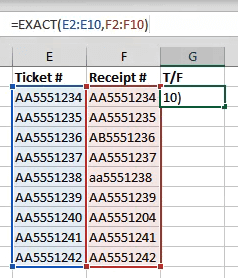
E2:E10 refers to the first column of values and F2:F10 refers to the column right next to it. Once we press Enter, Excel will compare the two values in each row and tell us if it’s a match (True) or not (False). Since we used ranges instead of just two cells, the formula will spill over into the cells below it and evaluate all the other rows.
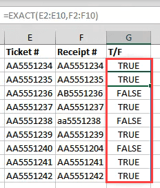
This method is limited though. It will only compare two cells that are on the same row. It won’t compare what’s in A2 with B3 for example. How do we do that? MATCH can help.
The MATCH Function
MATCH can be used to tell us where a match for a specific value is in a range of cells.
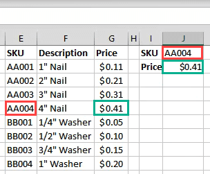
Let’s say we want to find out what row a specific SKU (Stock Keeping Unit) is in, in the example below.
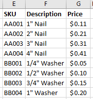
If we want to find what row AA003 is in, we would use the formula:
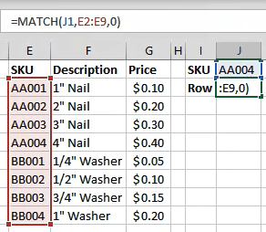
J1 refers to the cell with the value we want to match. E2:E9 refers to the range of values we’re searching through. The zero (0) at the end of the formula tells Excel to look for an exact match. If we were matching numbers, we could use 1 to find something less than our query or 2 to find something greater than our query.
But what if we wanted to find the price of AA003?
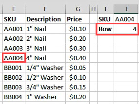
The VLOOKUP Function
The V in VLOOKUP stands for vertical. Meaning it can search for a given value in a column. What it can also do is return a value on the same row as the found value.
If you’ve got an Office 365 subscription in the Monthly channel, you can use the newer XLOOKUP. If you only have the semi-annual subscription it will be available to you in July 2020.
Let’s use the same inventory data and try to find the price of something.

Where we were looking for a row before, enter the formula:
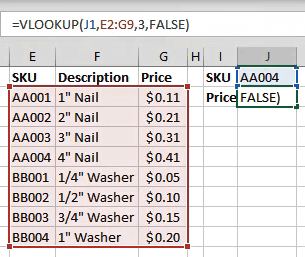
J1 refers to the cell with the value we’re matching. E2:G9 is the range of values we’re working with. But VLOOKUP will only look in the first column of that range for a match. The 3 refers to the 3rd column over from the start of the range.
So when we type a SKU in J1, VLOOKUP will find the match and grab the value from the cell 3 columns over from it. FALSE tells Excel what kind of match we’re looking for. FALSE means it must be an exact match where TRUE would tell it that it has to be a close match.
How Do I Find Matching Values in Two Different Sheets?
Each of the functions above can work across two different sheets to find matching values in Excel. We’re going to use the EXACT function to show you how. This can be done with almost any function. Not just the ones we covered here. There are also other ways to link cells between different sheets and workbooks.
Working on the Holders sheet, we enter the formula
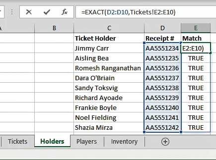
D2:D10 is the range we’ve selected on the Holders sheet. Once we put a comma after that, we can click on the Tickets sheet and drag and select the second range.
See how it references the sheet and range as Tickets!E2:E10? In this case each row matches, so the results are all True.
How Else Can I Use These Functions?
Once you master these functions for matching and finding things, you can start doing a lot of different things with them. Also take a look at using the INDEX and MATCH functions together to do something similar to VLOOKUP.
Have some cool tips on using Excel functions to find matching values in Excel? Maybe a question about how to do more? Drop us a note in the comments below.
Guy has been published online and in print newspapers, nominated for writing awards, and cited in scholarly papers due to his ability to speak tech to anyone, but still prefers analog watches. Read Guy’s Full Bio
Источник
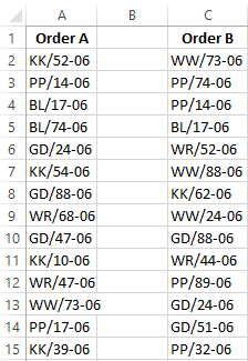
Comparison of two tables in Excel for finding matches in columns
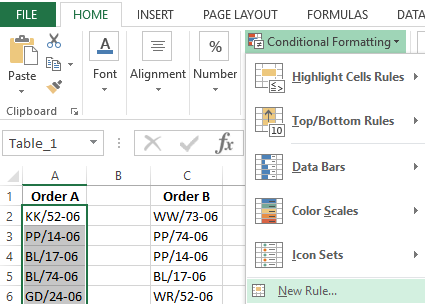
We have two tables of orders copied into one worksheet. You need to compare the data of the two tables in Excel and check which positions are in the first table but not in the second one. It makes no sense to manually compare the value of each cell.
Comparing two columns for finding matches in Excel
How can we compare values for two columns in Excel? To solve this task, we recommend using conditional formatting which quickly selects the color of positions that are only in one column. Worksheet with tables:
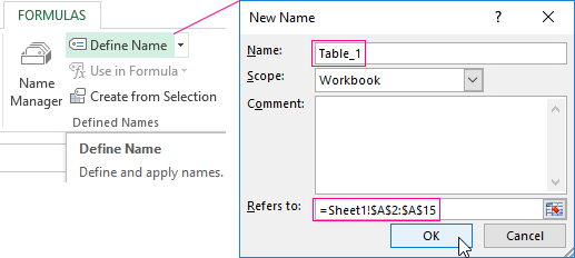
First, you need to name both tables. This makes it easier to understand which cell ranges are compared:
- Select the «FORMULAS» tool — «Defined Names» — «Define Name».
- Enter the value — Table_1 in the appeared window in the field «Name:»
- With the left mouse button click on the input field «Refers to:» and select the range: A2:A15. Then click OK.
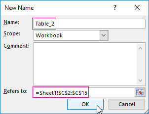
For the second list follow the same steps and just use another name — Table_2. And choose the range C2:C15 respectively.
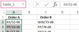
Helpful advice! Range names can be assigned more quickly by using the name field. It is located on the left of the formula row. Just select the ranges of cells, and in the name field enter the appropriate name for the range and press Enter.
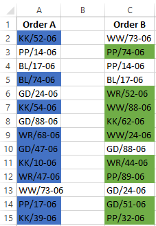
Now let’s use conditional formatting to compare two lists in Excel. We need to get the following result:
Positions that are in Table_1, but not in Table_2 will be displayed in green. At the same time, the items in Table 2 which don’t present in Table 1 will be highlighted in blue.
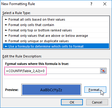
- Select the range of the first table A2:A15 and select the tool: «HOME»-«Conditional Formatting»-«New Rule»-«Use a formula to determine which cells to format:».

- Enter the formula in the input field:
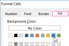
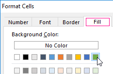
- Click on the «Format» button and specify a blue color on the «Fill» tab. Click OK in all windows.
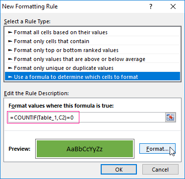
- Select the range of the first list C2:C15 and select the tool again – «HOME»-«Conditional Formatting»-«New Rule»-«Use a formula to determine which cells to format:».
- Enter the formula in the input field:
- Click on the «Format» button and specify the green color on the «Fill» tab. Click OK in all windows.
Principle of comparing the data of two columns in Excel
We used the COUNTIF function when defining conditions for formatting column cells. In this example, this function checks how many times the value of the second argument (for example, A2) occurs in the list of the first argument (for example, Table_2). If the number of times is 0, then the formula returns TRUE. In this case, the cell is assigned a custom format specified in the conditional formatting options. The reference in the second argument is relative, then all the cells of the selected range will be checked in turn (for example, A2: A15).
The second formula works similarly. The same principle can be applied to various similar tasks. For example, for comparing two prices in Excel and even on different worksheets.
Источник
MATCH function in Excel is used to find an exact match or the closest (less or more than the specified depending on the type of matching specified as an argument) value specified in the array or range of cells and returns the position number of the found element.
Examples of using the MATCH function in Excel
For example, we have a series of numbers from 1 to 10, written in cells B1:B10. Function =MATCH(3,B1,B10,0) will return the number 3, because the desired value is in cell B3, which is the third from the point of reference (cell B1).
This function is convenient for use in cases when it is necessary to return not the value contained in the desired cell, but its coordinate relative to the range in question. If arrays are used for constants, which can be represented as arrays of “key” — “value” elements, the FIND function returns a key value that is not explicitly specified.
For example, the array {«grapes»; «apple»; «pear»; «plum»} contains elements that can be represented as: 1 — «grapes», 2 — «apple», 3 — «pear», 4 — «plum «, Where 1, 2, 3, 4 — the keys, and the names of fruits — values. Then the function =MATCH(«apple»,{«grapes»,»apple»,»pear»,»plum»},0) returns the value 2, which is the key of the second element. The counting is performed not from 0 (zero), as it is implemented in many programming languages when working with arrays, but from 1.
MATCH function is rarely used independently. It is advisable to use it in conjunction with other functions, for example, INDEX.
Formula for finding inaccurate text matches in Excel
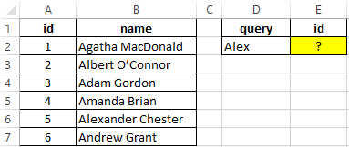
Example 1. Find the position of the first partial match of a string in a range of cells that store text values.
View source data table:
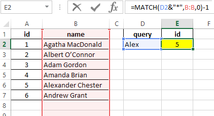
To find the position of a text string in a table, we use the following formula:
=MATCH(D2&»*»,B:B,0)-1
Argument Description:
- D2 & «*» is the sought value consisting of the last name specified in cell B2 and any number of other characters (“*”);
- B:B — reference to the column B: B, in which the search is performed;
- 0 — search for exact match.
A unit is subtracted from the obtained value to match the result with the id of the entry in the table.
Search example:
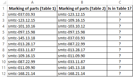
Comparison of two tables in Excel for the presence of discrepancies
Example 2. Excel stores two tables that appear to be the same at first glance. It was decided to compare one similar column of these tables for the presence of discrepancies. Implement a way to compare two cell ranges.
View of data table:
To compare the values in column B:B with the values from column A:A, use the following array formula (CTRL+SHIFT+ENTER):
MATCH function searches for a TRUE logical value in the array of logical values returned by the EXACT function (compares each element of the A2:A12 range with the value stored in cell B2 and returns an array of comparison results). If the MATCH function has found the value TRUE, the position of its first occurrence in the array will be returned. ISNA function will return FALSE if it does not accept the # N / A error value as an argument. In this case, the function IF returns the text string “is”, otherwise — “no”.
To calculate the remaining values, let us “stretch” the formula from cell C2 down to use the autocomplete function. As a result, we get:
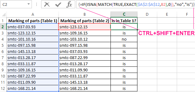
As you can see, the third elements of the lists do not match.
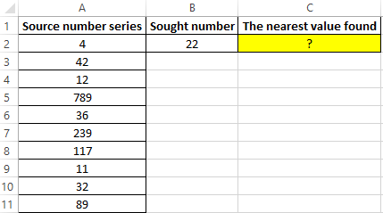
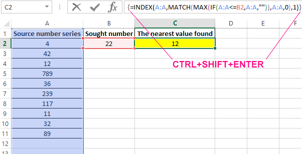
Finding the nearest greater knowledge in the range of Excel numbers
Example 3. Find the nearest smaller number to 22 in the range of numbers stored in an Excel spreadsheet column.
View source data table:
To search for the nearest larger value specified in the entire column A:A (a numerical series can be updated with new values) use the array formula (CTRL + SHIFT + ENTER):
MATCH function returns the position of the element in column A: A, which has the maximum value among the numbers that are greater than the number specified in cell B2. INDEX function returns the value stored in the found cell.
The result of the calculations:
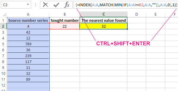
To search for the nearest smaller value, you only need to slightly change this formula and it should also be entered as an array (CTRL + SHIFT + ENTER):
Search results:
Features of using the function MATCH in Excel
The function has the following syntax entry:
=MATCH(Lookup_value,Lookup_array,[Match_type])
Argument Description:
- Lookup_value is a required argument that accepts textual, numeric values, as well as data of a logical and reference type, which is used as a search criterion (for comparing values or finding an exact match);
- Lookup_array is a required argument that accepts data of a reference type (references to a range of cells) or an array constant in which the search for the position of an element is performed according to the criteria specified by the first argument of the function;
- [Match_type] is an optional argument to fill in as a numeric value that defines how to search in a range of cells or an array. It can take the following values:
- -1 — search for the smallest nearest value given by the argument is_value in an ordered or descending array or range of cells.
- 0 — (by default) searches for the first value in an array or range of cells (not necessarily ordered), which is exactly the same as the value passed as the first argument.
- 1 — Search for the largest nearest value given by the first argument in an ordered array of cells in ascending order or range.
Download examples MATCH for finding occurring values in Excel
Notes:
- If a text string was passed as an argument to the Lookup_value, the MATCH function will return the position of the element in the array (if one exists) without case-sensitive characters. For example, the lines «New York» and «new york» are equivalent. To distinguish between registers, you can optionally use EXACT function.
- If the search using the function in question did not return results, the error code #N/A will be returned.
- If the argument [Match_type] is not explicitly specified or takes the number 0, wildcard characters can be used to search for partial match of text values (“?” Is the replacement of any single character, “*” is the replacement of any number of characters).
- If the data object passed as an argument to the Lookup_array contains two or more elements corresponding to the desired value, the position of the first occurrence of such an element will be returned.
The MATCH function is used to determine the position of a value in a range or array. For example, in the screenshot above, the formula in cell E6 is configured to get the position of the value in cell D6. The MATCH function returns 5 because the lookup value («peach») is in the 5th position in the range B6:B14:
=MATCH(D6,B6:B14,0) // returns 5
The MATCH function can perform exact and approximate matches and supports wildcards (* ?) for partial matches. There are 3 separate match modes (set by the match_type argument), as described below.
Note: the MATCH function will always return the first match. If you need to return the last match (reverse search) see the XMATCH function. If you want to return all matches, see the FILTER function.
MATCH only supports one-dimensional arrays or ranges, either vertical or horizontal. However, you can use MATCH to locate values in a two-dimensional range or table by giving MATCH the single column (or row) that contains the lookup value. You can even use MATCH twice in a single formula to find a matching row and column at the same time.
Frequently, the MATCH function is combined with the INDEX function to retrieve a value at a certain (matched) position. In other words, MATCH figures out the position, and INDEX returns the value at that position. For a detailed overview with simple examples, see How to use INDEX and MATCH.
Match type information
Match type is optional. If not provided, match_type defaults to 1 (exact or next smallest). When match_type is 1 or -1, it is sometimes referred to as an «approximate match». However, keep in mind that MATCH will always perform an exact match when possible, as noted in the table below:
| Match type | Behavior | Details |
|---|---|---|
| 1 | Approximate | MATCH finds the largest value less than or equal to the lookup value. The lookup array must be sorted in ascending order. |
| 0 | Exact | MATCH finds the first value equal to the lookup value. The lookup array does not need to be sorted. |
| -1 | Approximate | MATCH finds the smallest value greater than or equal to the lookup value. The lookup array must be sorted in descending order. |
| (omitted) | Approximate | When match_type is omitted, it defaults to 1 with behavior as explained above. |
Caution: Be sure to set match_type to zero (0) if you need an exact match. The default setting of 1 can cause MATCH to return results that look normal but are in fact incorrect. Explicitly providing a value for match_type, is a good reminder of what behavior is expected.
Exact match
When match_type is zero (0), MATCH performs an exact match only. In the example below, the formula in E3 is:
=MATCH(E2,B3:B11,0) // returns 4

In the formula above, the lookup value comes from cell E2. If the lookup value is hardcoded into the formula, it must be enclosed in double quotes («»), since it is a text value:
=MATCH("Mars",B3:B11,0)
Note: MATCH is not case-sensitive, so «Mars» and «mars» will both return 4.
Approximate match
When match_type is set to 1, MATCH will perform an approximate match on values sorted A-Z, finding the largest value less than or equal to the lookup value. In the example shown below, the formula in E3 is:
=MATCH(E2,B3:B11,1) // returns 5

Wildcard match
When match_type is set to zero (0), MATCH can use wildcards. In the example shown below, the formula in E3 is:
=MATCH(E2,B3:B11,0) // returns 6
This is equivalent to:
=MATCH("pq*",B3:B11,0)

INDEX and MATCH
The MATCH function is commonly used together with the INDEX function. The resulting formula is called «INDEX and MATCH». For example, in the screen below, INDEX and MATCH are used to return the cost of a code entered in cell F4. The formula in F5 is:
=INDEX(C5:C12,MATCH(F4,B5:B12,0)) // returns 150

In this example, MATCH is set up to perform an exact match. The MATCH function locates the code ABX-075 and returns its position (7) directly to the INDEX function as the row number. The INDEX function then returns the 7th value from the range C5:C12 as a final result. The formula is solved like this:
=INDEX(C5:C12,MATCH(F4,B5:B12,0))
=INDEX(C5:C12,7)
=150
See below for more examples of the MATCH function. For an overview of how to use INDEX and MATCH with many examples, see: How to use INDEX and MATCH.
Case-sensitive match
The MATCH function is not case-sensitive. However, MATCH can be configured to perform a case-sensitive match when combined with the EXACT function in a generic formula like this:
=MATCH(TRUE,EXACT(lookup_value,array),0))
The EXACT function compares every value in array with the lookup_value in a case-sensitive manner. This formula is explained with an INDEX and MATCH example here.
Notes
- MATCH is not case-sensitive.
- MATCH returns the #N/A error if no match is found.
- MATCH only works with text up to 255 characters in length.
- In case of duplicates, MATCH returns the first match.
- If match_type is -1 or 1, the lookup_array must be sorted as noted above.
- If match_type is 0, the lookup_value can contain the wildcards.
- The MATCH function is frequently used together with the INDEX function.
![]()
Download Article
![]()
Download Article
Excel remains one of the most powerful tools in the Microsoft Office Suite, but it can be understandably daunting as well. Fortunately, we have broken down one of Excel’s most essential features into just a few simple steps. This wikiHow article will teach you how to find matching values in two columns in Excel.
-
1
Select the columns you would like to compare. Using conditional formatting in Excel will allow you to automatically highlight any matching values across multiple columns. Click and drag your mouse over the columns you would like to compare.
- If the two columns are not side by side, simply hold down Ctrl and select whichever columns you need.
-
2
Click Conditional Formatting from the «Home» tab. This will open up a drop-down menu with various additional options.
Advertisement
-
3
Select Highlight Cells Rule and then Duplicate Values. This setting tells Excel that you want your conditional formatting to detect values that are duplicated (i.e., match) across your selected columns. [1]
-
4
Click OK on the pop-up window. After selecting your conditional formatting settings, Excel will show you a pop-up window. Ensure the window reads Duplicate in the left-hand box, and click «OK.»
- The other box in the pop-up window allows you to change the colors Excel uses to indicate duplicates. The default is «Light Red Fill with Dark Red Text», but you may choose whichever you prefer.
-
5
Identify the matching values. Excel will now highlight any duplicates with the formatting you chose in the previous pop-up box. Look for this colored formatting and identify any matches.
- Using conditional formatting to find matching values is a handy way to find matches that may not be in the same row.


Advertisement
-
1
Create a third column next to your two columns of data. The VLOOKUP function involves using a specific formula to find matching values. You’ll need a third column to input the formula and display any matches.
-
2
Enter the VLOOKUP formula into the first row of the third column. Assuming your data begins from the top-left corner of your spreadsheet, the formula is as follows: =VLOOKUP(B1,$A$1:$A$17,1,FALSE).
- The «17» in the formula indicates 17 rows of data. Change the number to fit however many rows of data you have.
- The «FALSE» value at the end of the formula is what tells Excel to look for an exact match in value. Replace it with «TRUE» to search for the nearest match that is less than or equal to the corresponding data point (represented in this case by B1). [2]
- Just entering «=VLOOKUP» in Excel will pull up the full formula, which you can reference in populating each field with the necessary info.
-
3
Copy the VLOOKUP formula all the way down. Drag down from the corner of the first box to your final row of data to copy the formula. Excel will automatically change the first value to the corresponding data point in that row. [3]
-
4
Look for matching values in your third column. If there are any matching values, they will display as a number in your spreadsheet’s third column. If there are no matching values, the VLOOKUP formula will simply turn up «#N/A».


Advertisement
-
1
Create a third column next to your two columns of data. This method involves using a specific formula to find matching values. You’ll need a third column to input the formula and display its results.
-
2
Enter the TRUE/FALSE formula into the third column. Assuming your data begins from the top-left corner of your spreadsheet, the formula is as follows: =A1=B1.
-
3
Copy the formula all the way down. Drag down from the corner of the first box to your final row of data to copy the formula. Excel will automatically change the values to the corresponding data points in that row.
-
4
Look for a «TRUE» or «FALSE» assessment in the third column. Matching values will turn up a «TRUE» value. If there is no match, the box in the third column will read «FALSE.»


Advertisement
Ask a Question
200 characters left
Include your email address to get a message when this question is answered.
Submit
Advertisement
About This Article
Article SummaryX
1. Use conditional formatting to highlight matching values.
2. Use VLOOKUP or a TRUE/FALSE formula to display matching values in a new column.
Did this summary help you?
Thanks to all authors for creating a page that has been read 40,151 times.
Is this article up to date?
Different Methods to Match Data in Excel
There are various methods to match data in Excel. For example, suppose we want to compare the data in the same column, e.g., check for duplicity. In that case, we can use “Conditional Formatting” from the “Home” tab. On the other hand, if we want to match the data in two or more different columns, we can use conditional functions like the IF function.
Table of contents
- Different Methods to Match Data in Excel
- #1 – Match Data Using VLOOKUP Function
- #2 – Match Data Using INDEX + MATCH Function
- #3 – Create Your Own Lookup Value
- Recommended Articles
- Method #1 – Using Vlookup Function
- Method #2 – Using Index + Match Function
- Method #3 – Create Your Own Lookup Value
Now, let us discuss each of the methods in detail.
You can download this Match Data Excel Template here – Match Data Excel Template
#1 – Match Data Using VLOOKUP Function
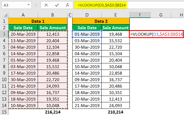
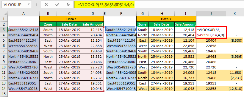
The VLOOKUP function is not only used to get the required information from the data table. It can also be used as a reconciliation tool. When reconciling or matching the data, the VLOOKUP formula leads the table.
- For example, look at the below table.

- We have two data tables here. The first is Data 1. The second is Data 2.
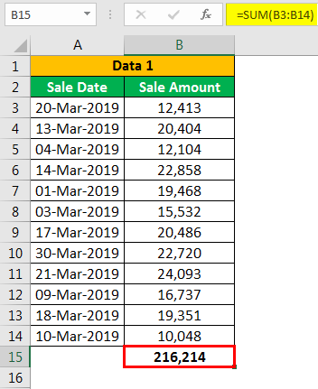
Now, we need to reconcile whether the data in the two tables match. The first way of comparing the data is the SUM function in excel to two tables to get the total sales.
Data 1 – Table

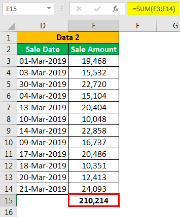
Data 2 – Table

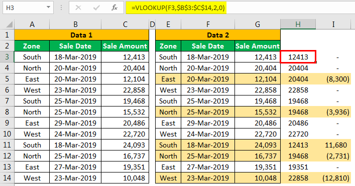
- We have applied the SUM function for the table’s Sale Amount column. In the beginning, we have got the difference in values. The Data 1 table shows the total sales of 2,16,214, and the Data 2 table shows 2,10,214.
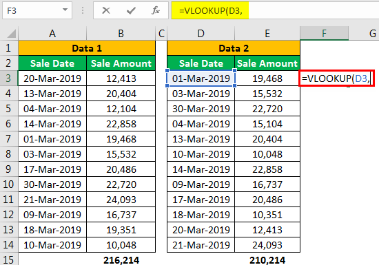
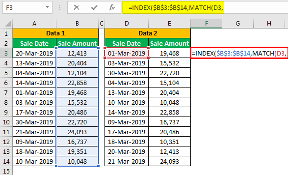
Now, we need to examine this in detail. So, let us apply the VLOOKUP function for each date.

- Select the table array as Data 1 range.

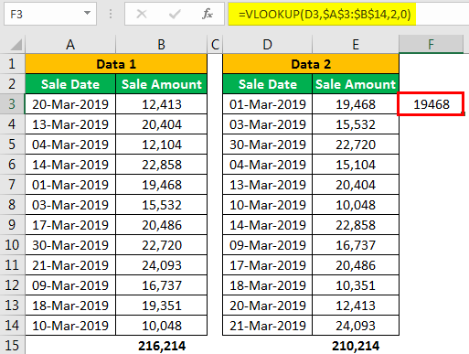
- We need the data from the second column, and the range of LOOKUP is FALSE, i.e., exact match.

- The output is given below:

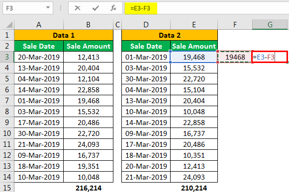
- First, we must deduct the original value from the next cell’s arrival value.

- After deducting, we get the result as zero.

- We must copy and paste the formula to all the cells to get the variance values.

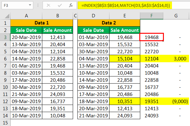
- In cells G6 and G12, we got the differences.


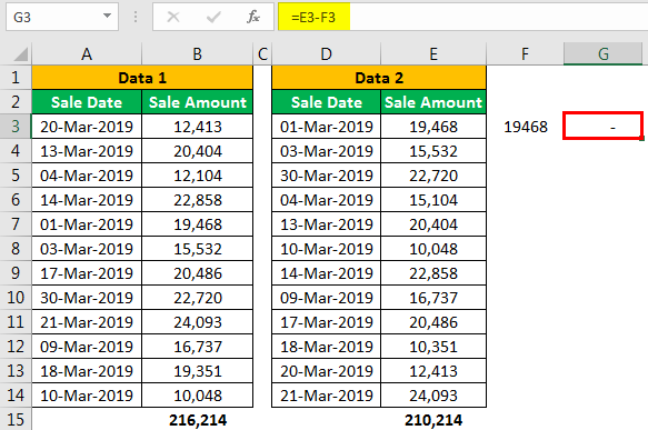
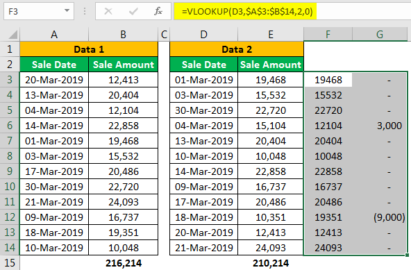
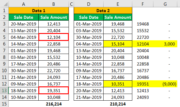
In Data 1, we have 12,104 for 04-Mar-2019. However, in Data 2, we have 15,104 for the same date, so there is a difference of 3,000.
Similarly, for 18-Mar-2019 in Data 1, we have 19,351. In Data 2, we have 10,351, so the difference is 9,000.
#2 – Match Data Using INDEX + MATCH Function
For the same data, we can use the INDEX + MATCH function. We can use this as an alternative to the VLOOKUP functionTo reference data in columns from right to left, we can combine the index and match functions, which is one of the best Excel alternatives to Vlookup.read more.
The INDEX function is used to get the value from the selected column based on the row number provided. We need to use the MATCH functionThe MATCH function looks for a specific value and returns its relative position in a given range of cells. The output is the first position found for the given value. Being a lookup and reference function, it works for both an exact and approximate match. For example, if the range A11:A15 consists of the numbers 2, 9, 8, 14, 32, the formula “MATCH(8,A11:A15,0)” returns 3. This is because the number 8 is at the third position.
read more based on the LOOKUP value to give the row number.
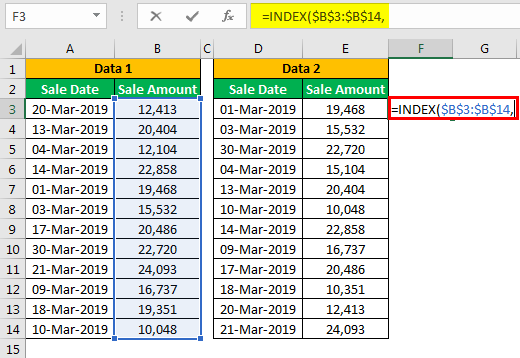
We must Open INDEX functionThe INDEX function in Excel helps extract the value of a cell, which is within a specified array (range) and, at the intersection of the stated row and column numbers.read more in the F3 cell.

Then, select the array as a result column range, B2 to B14.
Open the MATCH function as the next argument to get the row number.
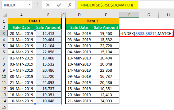
Select the LOOKUP value as a D3 cell.
Next, select the lookup array as the “Sales Date” column in Data 1.
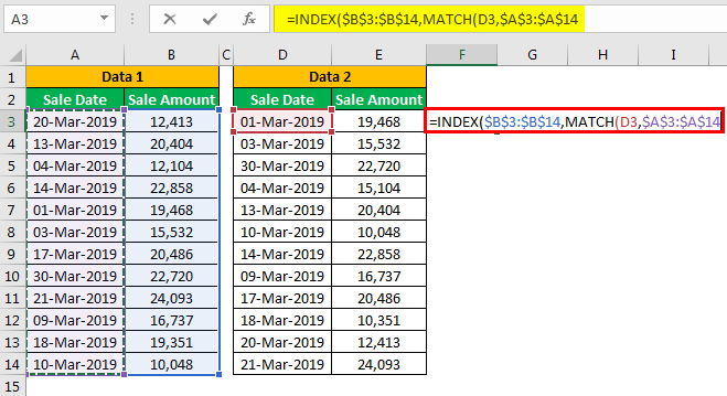
In the match type, select “0 – Exact Match.”

Now, close two brackets and press the “Enter” key to get the result.
It also gives the same result as VLOOKUP. Since we have used the same data, we got the numbers as it is.
#3 – Create Your Lookup Value
Now, we have seen how to match data using Excel functions. Now, we will see the different scenarios in real-time. For this example, look at the below data.
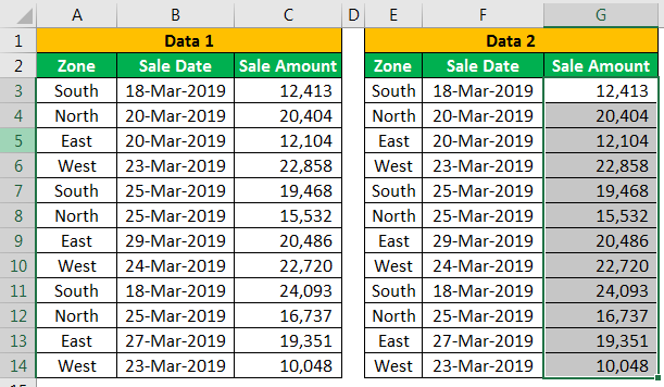
As shown above, we have zone-wise and date-wise sales data in the above data. Therefore, we need to perform the data matching process again. But, first, let us apply the VLOOKUP function as per the previous example.
We got many variances. Let us examine each case by case.
In cell I5, we got a variance of 8,300. Let us look at the main table.
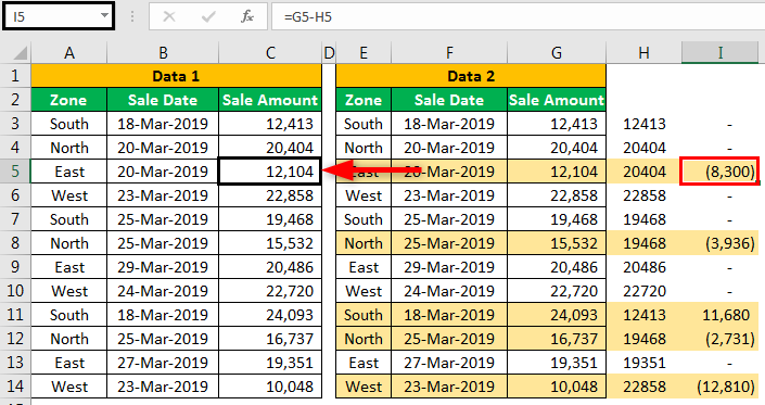
Even though the main table value is 12,104, we got the value of 20,404 from the VLOOKUP function. That is because VLOOKUP can return the first found LOOKUP value.
In this case, our LOOKUP value is a date of 20-Mar-2019. In the above cell for the “North” zone for the same date, we have a value of 20,404, so VLOOKUP has returned this value for the “East” zone.
To overcome this issue, we need to create unique LOOKUP values. For example, combine Zone, Date, and Sales Amount in Data 1 and Data 2.
Data 1 – Table
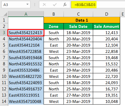
Data 2 – Table
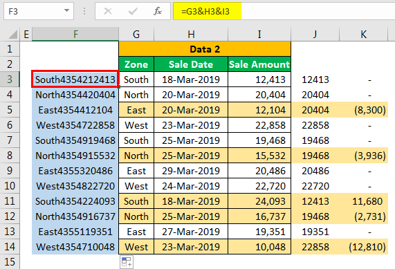
We have created unique values for each zone with the combined value of “Zone,” “Sale Date,” and “Sale Amount.”
Using these unique values, let us apply the VLOOKUP function.
Apply the formula to all the cells. We will get the variance of zero in all the cells.

Like this, by using Excel functions, we can match the data and find the variances. First, however, we need to look at the duplicates in the LOOKUP value for accurate reconciliationReconciliation is the process of comparing account balances to identify any financial inconsistencies, discrepancies, omissions, or even fraud. At the end of any accounting period, reconciliation involves matching balances and ensuring that debits (credits) from one account for one transaction is same as the credit (debits) to another account for the same transaction.read more before applying the formula. The above example is the best illustration of duplicate values in the LOOKUP value. We need to create our unique LOOKUP values in such scenarios and arrive at the result.
Recommended Articles
This article is a guide to Match Data in Excel. We discuss matching data in Excel using the VLOOKUP function, INDEX + MATCH function, and our LOOKUP value with a downloadable Excel template. You may learn more about Excel from the following articles: –
- What is VBA Match?
- Vlookup to the Left
- VLOOKUP Table Array
- Lookup Excel Table
Excel has a lot of functions – about 450+ of them.
And many of these are simply awesome. The amount of work you can get done with a few formulas still surprises me (even after having used Excel for 10+ years).
And among all these amazing functions, the INDEX MATCH functions combo stands out.
I am a huge fan of INDEX MATCH combo and I have made it pretty clear many times.
I even wrote an article about Index Match Vs VLOOKUP which sparked a little bit of debate (you can check the comments section for some firework).
And today, I am writing this article solely focussed on Index Match to show you some simple and advanced scenarios where you can use this powerful formula combo and get the work done.
Note: There are other lookup formulas in Excel – such as VLOOKUP and HLOOKUP and these are great. Many people find VLOOKUP to be easier to use (and that’s true as well). I believe INDEX MATCH is a better option in many cases. But since people find it difficult, it gets used less. So I am trying to simplify it using this tutorial.
Now before I show you how the combination of INDEX MATCH is changing the world of analysts and data scientists, let me first introduce you to the individual parts – INDEX and MATCH functions.
INDEX Function: Finds the Value-Based on Coordinates
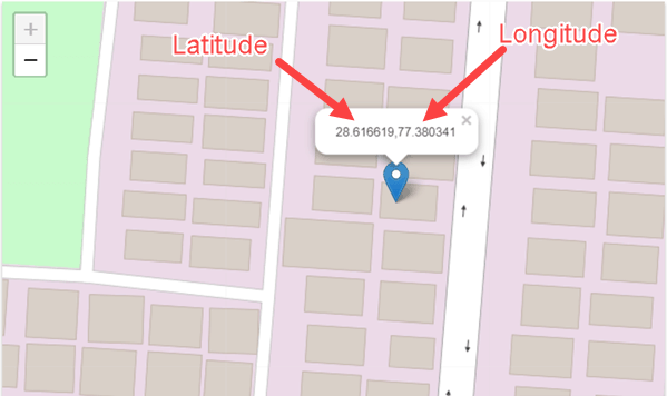
The easiest way to understand how Index function works is by thinking of it as a GPS satellite.
As soon as you tell the satellite the latitude and longitude coordinates, it will know exactly where to go and find that location.
So despite having a mind-boggling number of lat-long combinations, the satellite would know exactly where to look.
I quickly did a search for my work location and this is what I got.
Anyway, enough of geography.
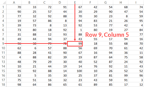
Just like a satellite needs latitude and longitude coordinates, the INDEX function in Excel would need the row and column number to know what cell you’re referring to.
And that’s Excel INDEX function in a nut-shell.
So let me define it in simple words for you.
The INDEX function will use the row number and column number to find a cell in the given range and return the value in it.
All by itself, INDEX is a very simple function, with no utility. After all, in most cases, you are not likely to know the row and column numbers.
But…
The fact that you can use it with other functions (hint: MATCH) that can find the row number and the column number makes INDEX an extremely powerful Excel function.
Below is the syntax of the INDEX function:
=INDEX (array, row_num, [col_num])
=INDEX (array, row_num, [col_num], [area_num])
- array – a range of cells or an array constant.
- row_num – the row number from which the value is to be fetched.
- [col_num] – the column number from which the value is to be fetched. Although this is an optional argument, but if row_num is not provided, it needs to be given.
- [area_num] – (Optional) If array argument is made up of multiple ranges, this number would be used to select the reference from all the ranges.
INDEX function has 2 syntaxes (just FYI).
The first one is used in most cases. The second one is used in advanced cases only (such as doing a three-way lookup) which we will cover in one of the examples later in this tutorial.
But if you’re new to this function, just remember the first syntax.
Below is a video that explains how to use the INDEX function
MATCH Function: Finds the Position baed on a Lookup Value
Going back to my previous example of longitude and latitude, MATCH is the function that can find these positions (in the Excel spreadsheet world).
In simple language, the Excel MATCH function can find the position of a cell in a range.
And on what basis would it find a cell’s position?
Based on the lookup value.
For example, if you have a list as shown below and you want to find the position of the name ‘Mark’ in it, then you can use the MATCH function.
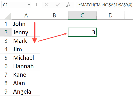
The function returns 3, as that’s the position of the cell with the name Mark in it.
MATCH function starts looking from top to bottom for the lookup value (which is ‘Mark’) in the specified range (which is A1:A9 in this example). As soon as it finds the name, it returns the position in that specific range.
Below is the syntax of the MATCH function in Excel.
=MATCH(lookup_value, lookup_array, [match_type])
- lookup_value – The value for which you are looking for a match in the lookup_array.
- lookup_array – The range of cells in which you are searching for the lookup_value.
- [match_type] – (Optional) This specifies how excel should look for a matching value. It can take three values -1, 0 , or 1.
Understanding Match Type Argument in MATCH Function
There is one additional thing you need to know about the MATCH function, and it’s about how it goes through the data and finds the cell position.
The third argument of the MATCH function can be 0, 1 or -1.
Below is an explanation of how these arguments work:
- 0 – this will look for an exact match of the value. If an exact match is found, the MATCH function will return the cell position. Else, it will return an error.
- 1 – this finds the largest value that is less than or equal to the lookup value. For this to work, your data range needs to be sorted in ascending order.
- -1 – this finds the smallest value that is greater than or equal to the lookup value. For this to work, your data range needs to be sorted in descending order.
Below is a video that explains how to use the MATCH function (along with the match type argument)
To summarize and put it in simple words:
- INDEX needs the cell position (row and column number) and gives the cell value.
- MATCH finds the position by using a lookup value.
Let’s Combine Them to Create a Powerhouse (INDEX + MATCH)
Now that you have a basic understanding of how INDEX and MATCH functions work individually, let’s combine these two and learn about all the wonderful things it can do.
To understand this better, I have a few examples that use the INDEX MATCH combination.
I will start with a simple example and then show you some advanced use cases as well.
Click here to download the example file
Example 1: A simple Lookup Using INDEX MATCH Combo
Let’s do a simple lookup with INDEX/MATCH.
Below is a table where I have the marks for ten students.
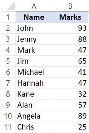
From this table, I want to find the marks for Jim.
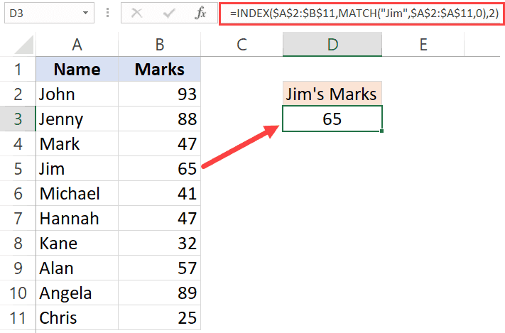
Below is the formula that can easily do this:
=INDEX($A$2:$B$11,MATCH("Jim",$A$2:$A$11,0),2)
Now, if you’re thinking this can easily be done using a VLOOKUP function, you’re right! This is not the best use of INDEX MATCH awesomeness. Despite the fact that I am a fan of INDEX MATCH, it is a little more difficult than VLOOKUP. If fetching data from a column on the right is all you want to do, I recommend you use VLOOKUP.
The reason I have shown this example, which can also easily be done with VLOOKUP is to show you how INDEX MATCH works in a simple setting.
Now let me show a benefit of INDEX MATCH.
Suppose you have the same data, but instead of having it in columns, you have it in rows (as shown below).

You know what, you can still use INDEX MATCH combo to get Jim’s marks.
Below is the formula that will give you the result:
=INDEX($B$1:$K$2,2,MATCH(“Jim”,$B$1:$K$1,0))
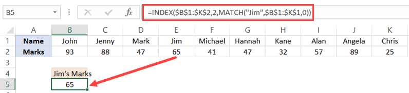
Note that you need to change the range and switch the row/column parts to make this formula work for horizontal data as well.
This can’t be done with VLOOKUP, but you can still do this easily with HLOOKUP.
INDEX MATCH combination can easily handle horizontal as well as vertical data.
Click here to download the example file
Example 2: Lookup to the Left
It’s more common than you think.
A lot of times, you may be required to fetch the data from a column which is to the left of the column that has the lookup value.
Something as shown below:
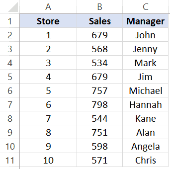
To find out Michael’s sales, you will have to do a lookup on the left.
If you’re thinking VLOOKUP, let me stop your right there.
VLOOKUP is not made to look for and fetch the values on the left.
Can you still do it using VLOOKUP?
Yes, you can!
But that can turn into a long and ugly formula.
So if you want to do a lookup and fetch data from the columns on the left, you are better off using INDEX MATCH combo.
Below is the formula that will get Michael’s sales number:
=INDEX($A$2:$C$11,MATCH("Michael",C2:C11,0),2)
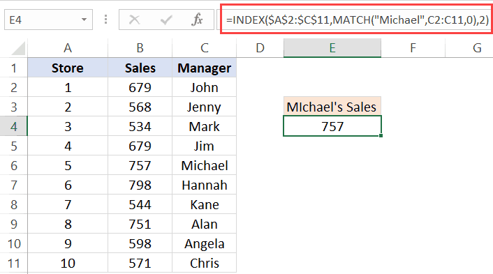
Another point here for INDEX MATCH. VLOOKUP can fetch the data only from the columns that are to the right of the column that has the lookup value.
Example 3: Two Way Lookup
So far, we have seen the examples where we wanted to fetch the data from the column adjacent to the column that has the lookup value.
But in real life, the data often spans through multiple columns.
INDEX MATCH can easily handle a two-way lookup.
Below is a dataset of the student’s marks in three different subjects.
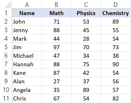
If you want to quickly fetch the marks of a student in all three subjects, you can do that with INDEX MATCH.
The below formula will give you the marks for Jim for all the three subjects (copy and paste in one cell and drag to fill other cells or copy and paste on other cells).
=INDEX($B$2:$D$11,MATCH($F$3,$A$2:$A$11,0),MATCH(G$2,$B$1:$D$1,0))

Let me quickly also explain this formula.
INDEX formula uses B2:D11 as the range.
The first MATCH uses the name (Jim in cell F3) and fetches the position of it in the names column (A2:A11). This becomes the row number from which the data needs to be fetched.
The second MATCH formula uses the subject name (in cell G2) to get the position of that specific subject name in B1:D1. For example, Math is 1, Physics is 2 and Chemistry is 3.
Since these MATCH positions are fed into the INDEX function, it returns the score based on the student name and subject name.
This formula is dynamic, which means that if you change the student name or the subject names, it would still work and fetch the correct data.
One great thing about using INDEX/MATCH is that even if you interchange the names of the subjects, it will continue to give you the correct result.
Example 4: Lookup Value From Multiple Column/Criteria
Suppose you have a dataset as shown below and you want to fetch the marks for ‘Mark Long’.

Since the data is in two columns, I can’t a lookup for Mark and get the data.
If I do it that way, I am going to get the marks data for Mark Frost and not Mark Long (because the MATCH function will give me the result for the MARK it meets).
One way of doing this is to create a helper column and combine the names. Once you have the helper column, you can use VLOOKUP and get the marks data.
If you’re interested in learning how to do this, read this tutorial on using VLOOKUP with multiple criteria.
But with INDEX/MATCH combo, you don’t need a helper column. You can create a formula that handles multiple criteria in the formula itself.
The below formula will give the result.
=INDEX($C$2:$C$11,MATCH($E$3&"|"&$F$3,$A$2:A11&"|"&$B$2:$B$11,0))

Let me quickly explain what this formula does.
The MATCH part of the formula combines the lookup value (Mark and Long) as well as the entire lookup array. When $A$2:A11&”|”&$B$2:$B$11 is used as the lookup array, it actually checks the lookup value against the combined string of first and last name (separated by the pipe symbol).
This ensures that you get the right result without using any helper columns.
You can do this kind of lookup (where there are multiple columns/criteria) with VLOOKUP as well, but you need to use a helper column. INDEX MATCH combo makes it slightly easy to do this without any helper columns.
Example 5: Get Values from Entire Row/Column
In the examples above, we have used the INDEX function to get value from a specific cell. You provide the row and column number, and it returns the value in that specific cell.
But you can do more.
You can also use the INDEX function to get the values from an entire row or column.
And how can this be useful you ask!
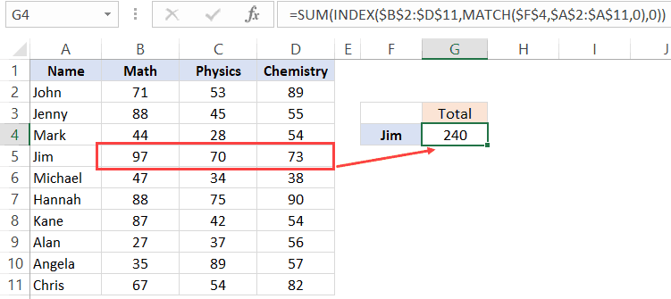
Suppose you want to know the total score of Jim in all the three subjects.
You can use the INDEX function to first get all the marks of Jim and then use the SUM function to get a total.
Let’s see how to do this.
Below I have the scores of all the students in three subjects.
The below formula will give me the total score of Jim in all the three subjects.
=SUM(INDEX($B$2:$D$11,MATCH($F$4,$A$2:$A$11,0),0))
Let me explain how this formula works.
The trick here is to use 0 as the column number.
When you use 0 as the column number in the INDEX function, it will return all the row values. Similarly, if you use 0 as the row number, it will return all the values in the column.
So the below part of the formula returns an array of values – {97, 70, 73}
INDEX($B$2:$D$11,MATCH($F$4,$A$2:$A$11,0),0)
If you just enter this above formula in a cell in Excel and hit enter, you will see a #VALUE! error. This is because it’s not returning a single value, but an array of value.
But don’t worry, the array of values are still there. You can check this by selecting the formula and press the F9 key. It will show you the result of the formula which in this case is an array of three value – {97, 70, 73}
Now, if you wrap this INDEX formula in the SUM function, it will give you the sum of all the marks scored by Jim.
You can also use the same to get the highest, lowest and average marks of Jim.
Just like we have done this for a student, you can also do this for a subject. For example, if you want the average score in a subject, you can keep the row number as 0 in the INDEX formula and it will give you all the column values of that subject.
Click here to download the example file
Example 6: Find the Student’s Grade (Approximate Match Technique)
So far, we have used the MATCH formula to get the exact match of the lookup value.
But you can also use it to do an approximate match.
Now, what the hell is Approximate Match?
Let me explain.
When you’re looking for stuff such as names or ids, you’re looking for an exact match. But sometimes, you need to know the range in which your lookup values lie. This is usually the case with numbers.
For example, as a class teacher, you may want to know what’s the grade of each student in a subject, and the grade is decided based on the score.
Below is an example, where I want the grade for all the students and the grading is decided based on the table on the right.
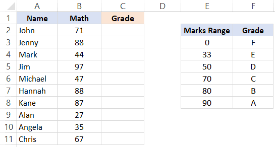
So if a student gets less than 33, the grade is F and if he/she gets less than 50 but more than 33, it’s E, and so on.
Below is the formula that will do this.
=INDEX($F$3:$F$8,MATCH(B2,$E$3:$E$8,1),1)
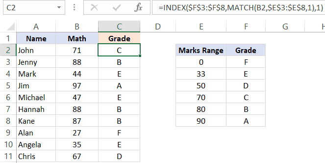
Let me explain how this formula works.
In the MATCH function, we have used 1 as the [match_type] argument. This argument will return the largest value that is less than or equal to the lookup value.
This means that the MATCH formula goes through the marks range, and as soon as it finds a marks range that is equal to or less than the lookup marks value, it will stop there and return its position.
So if the lookup mark value is 20, the MATCH function would return 1 and if it’s 85, it would return 5.
And the INDEX function uses this position value to get the grade.
IMPORTANT: For this to work, your data needs to be sorted in ascending order. If it’s not, you can get wrong results.
Note that the above can also be done using below VLOOKUP formula:
=VLOOKUP(B2,$E$3:$F$8,2,TRUE)
But MATCH function can go a step further when it comes to approximate match.
You can also have a descending data and can use INDEX MATCH combo to find the result. For example, if I change the order of the grade table (as shown below), I can still find the grades of the students.
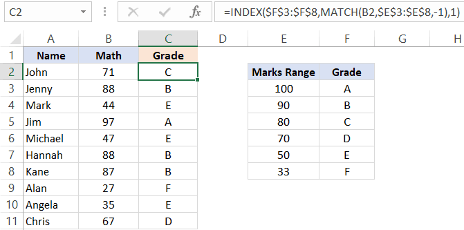
To do this, all I have to do is change the [match_type] argument to -1.
Below is the formula that I have used:
=INDEX($F$3:$F$8,MATCH(B2,$E$3:$E$8,-1),1)
VLOOKUP can also do an approximate match but only when data is sorted in ascending order(but it doesn’t work if the data is sorted in descending order).
Example 7: Case Sensitive Lookups
So far all the lookups we have done have been case insensitive.
This means that whether the lookup value was Jim or JIM or jim, it didn’t matter. You’ll get the same result.
But what if you want the lookup to be case sensitive.
This is usually the case when you have large data sets and a possibility of repetition or distinct names/ids (with the only difference being the case)
For example, suppose I have the following data set of students where there are two students with the name Jim (the only difference being that one is entered as Jim and another one as jim).

Note that there are two students with the same name – Jim (cell A2 and A5).
Since a normal lookup wouldn’t work, you need to do a case sensitive lookup.
Below is the formula that will give you the right result. Since this is an array formula, you need to use Control + Shift + Enter.
=INDEX($B$2:$B$11,MATCH(TRUE,EXACT(D3,A2:A11),0),1)

Let me explain how this formula works.
The EXACT function checks for an exact match of the lookup value (which is ‘jim’ in this case). It goes through all the names and returns FALSE if it isn’t a match and TRUE if it’s a match.
So the output of the EXACT function in this example is – {FALSE;FALSE;FALSE;TRUE;FALSE;FALSE;FALSE;FALSE;FALSE;FALSE}
Note that there is only one TRUE, which is when the EXACT function found a perfect match.
The MATCH function then finds the position of TRUE in the array returned by the EXACT function, which is 4 in this example.
Once we have the position, the INDEX function uses it to find the marks.
Example 8: Find the Closest Match
Let’s get a little advanced now.
Suppose you have a dataset where you want to find the person who has the work experience closest to the required experience (mentioned in cell D2).
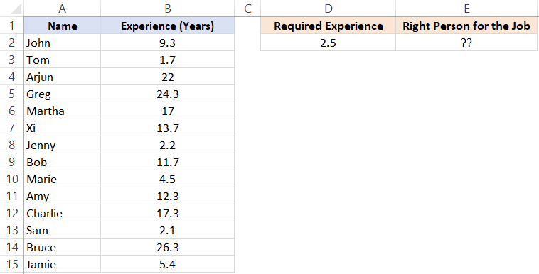
While lookup formulas are not made to do this, you can combine it with other functions (such as MIN and ABS) to get this done.
Below is the formula that will find the person with the experience closest to the required one and return the name of the person. Note that the experience needs to be closest (which can be either less or more).
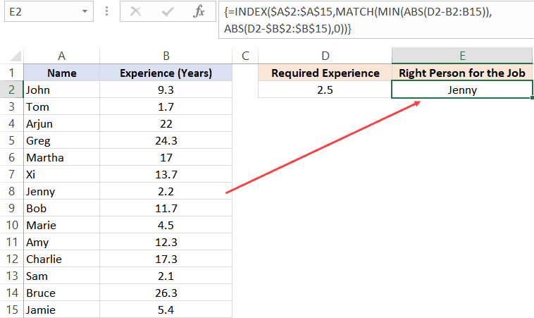
=INDEX($A$2:$A$15,MATCH(MIN(ABS(D2-B2:B15)),ABS(D2-$B$2:$B$15),0))
Since this is an array formula, you need to use Control + Shift + Enter.
The trick in this formula is to change the lookup value and lookup array to find the minimum experience difference in required and actual values.
Before I explain the formula, let’s understand how you would do it manually.
You will go through each cell in column B and find the difference in the experience between what is required and the one that a person has. Once you have all the differences, you will find the one which is minimum and fetch the name of that person.
This is exactly what we are doing with this formula.
Let me explain.
The lookup value in the MATCH formula is MIN(ABS(D2-B2:B15)).
This part gives you the minimum difference between the given experience (which is 2.5 years) and all the other experiences. In this example, it returns 0.3
Note that I have used ABS to make sure I am looking for the closest (which can be more or less than the given experience).
Now, this minimum value becomes our lookup value.
The lookup array in the MATCH function is ABS(D2-$B$2:$B$15).
This gives us an array of numbers from which 2.5 (the required experience) has been subtracted.
So now we have a lookup value (0.3) and a lookup array ({6.8;0.8;19.5;21.8;14.5;11.2;0.3;9.2;2;9.8;14.8;0.4;23.8;2.9})
MATCH function finds the position of 0.3 in this array, which is also the position of the person’s name who has the closest experience.
This position number is then used by the INDEX function to return the name of the person.
Related Read: Find the Closest Match in Excel (examples using lookup formulas)
Click here to download the example file
Example 9: Use INDEX MATCH with Wildcard Characters
If you want to look up a value when there is a partial match, then you need to use wildcard characters.
For example, below is a dataset of company name and their market capitalizations and you want to want to get the market cap. data for the three companies on the right.
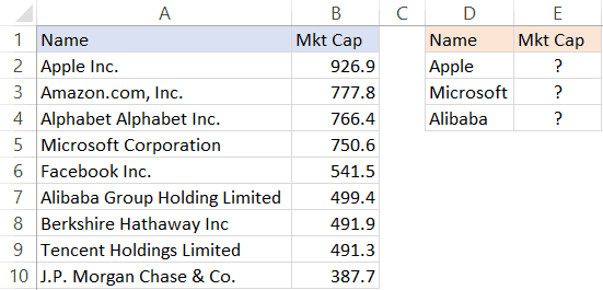
Since these are not exact matches, you can’t do a regular lookup in this case.
But you can still get the right data by using an asterisk (*), which is a wildcard character.
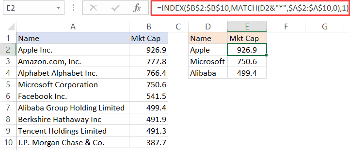
Below is the formula that will give you the data by matching the company names from the main column and fetching the market cap figure for it.
=INDEX($B$2:$B$10,MATCH(D2&”*”,$A$2:$A$10,0),1)
Let me explain how this formula works.
Since there is no exact match of lookup values, I have used D2&”*” as the lookup value in the MATCH function.
An asterisk is a wildcard character that represents any number of characters. This means that Apple* in the formula would mean any text string that starts with the word Apple and can have any number of characters after it.
So when Apple* is used as the lookup value and the MATCH formula looks for it in column A, it returns the position of ‘Apple Inc.’, as it starts with the word Apple.
You can also use wildcard characters to find text strings where the lookup value is in between. For example, if you use *Apple* as the lookup value, it will find any string that has the word apple anywhere in it.
Note: This technique works well when you only have one instance of matching. But if you have multiple instances of matching (for example Apple Inc and Apple Corporation, then the MATCH function would return the position of the first matching instance only.
Example 10: Three Way Lookup
This is an advanced use of INDEX MATCH, but I will still cover it to show you the power of this combination.
Remember I said that INDEX function has two syntaxes:
=INDEX (array, row_num, [col_num])
=INDEX (array, row_num, [col_num], [area_num])
So far in all our examples, we have only used the first one.
But for a three-way lookup, you need to use the second syntax.
Let me first explain what a three-way look means.
In a two-way lookup, we use the INDEX MATCH formula to get the marks when we have the student’s name and the subject name. For example, fetching the marks of Jim in Math is a two-way lookup.
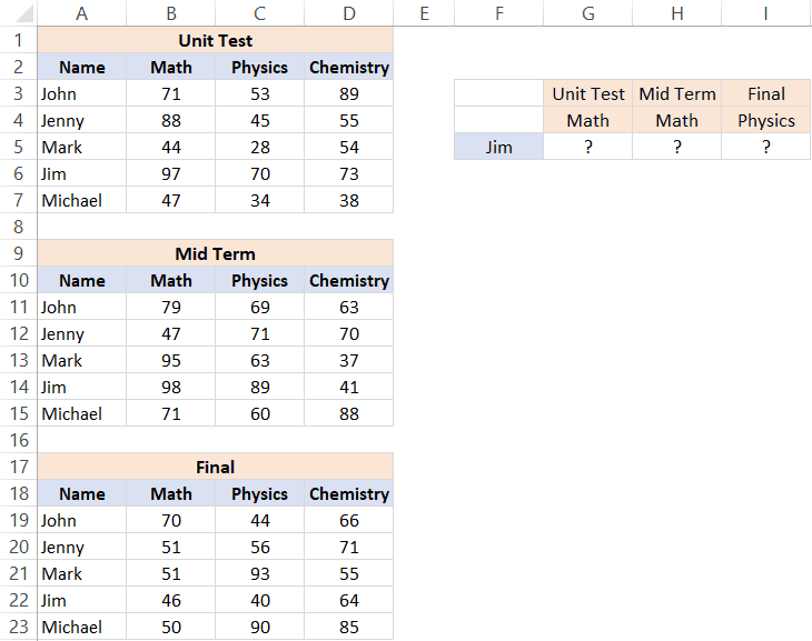
A three-way look would add another dimension to it. For example, suppose you have a dataset as shown below and you want to know the score of Jim in Math in Mid-term exam, then this would be three-way lookup.
Below is the formula that will give the result.
=INDEX(($B$3:$D$7,$B$11:$D$15,$B$19:$D$23),MATCH($F$5,$A$3:$A$7,0),MATCH(G$4,$B$2:$D$2,0),(IF(G$3="Unit Test",1,IF(G$3="Mid Term",2,3))))
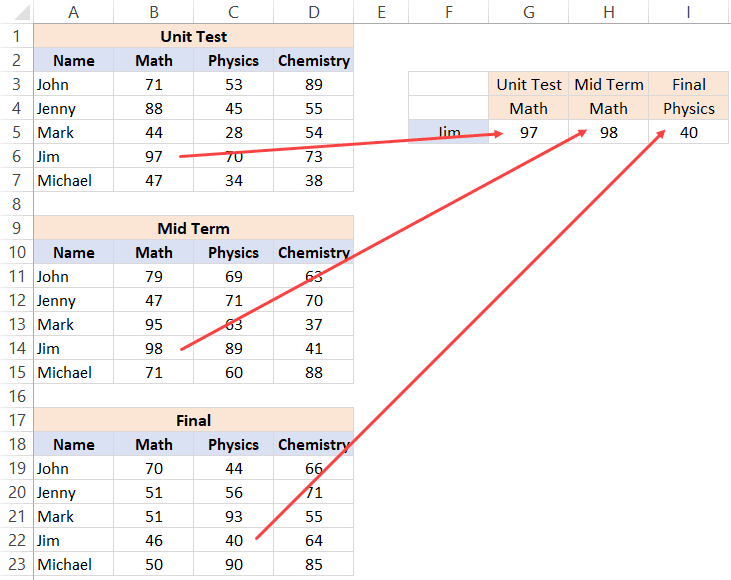
The above formula checked for three things – the name of the student, the subject, and the exam. After it finds the right value, it returns it in the cell.
Let me explain how this formula works by breaking down the formula into parts.
- array – ($B$3:$D$7,$B$11:$D$15,$B$19:$D$23): Instead of using a single array, in this case, I have used three arrays within parenthesis.
- row_num – MATCH($F$5,$A$3:$A$7,0): MATCH function is used to find the position of the student’s name in cell $F$5 in the list of student’s name.
- col_num – MATCH(G$4,$B$2:$D$2,0): MATCH function is used to find the position of the subject name in cell $B$2 in the list of subject’s name.
- [area_num] – IF(G$3=”Unit Test”,1,IF(G$3=”Mid Term”,2,3)): The area number value tells the INDEX function which of the three arrays to use to fetch the value. If the exam is Unit Term, the IF function would return 1 and the INDEX function would use the first array to fetch the value. If the exam is Mid-term, the IF formula would return 2, else it will return 3.
This is an advanced example of using INDEX MATCH, and you’re unlikely to find a situation when you have to use this. But it’s still good to know what Excel formulas can do.
Click here to download the example file
Why is INDEX/MATCH Better than VLOOKUP?
OR Is it?
Yes, it is – in most cases.
I will present my case in a while.
But before I do that, let me say this – VLOOKUP is an extremely useful function and I love it. It can do a lot of things in Excel and I use it every now and then myself. Having said that, it doesn’t mean that there can’t be anything better, and INDEX/MATCH (with more flexibility and functionalities) is better.
So if you want to do some basic lookup, you’re better off using VLOOKUP.
INDEX/MATCH is VLOOKUP on steroids. And once you learn INDEX/MATCH, you might always prefer using it (especially because of the flexibility it has).
Without stretching it too far, let me quickly give you the reasons why INDEX/MATCH is better than VLOOKUP.
INDEX/MATCH can look to the Left (as well as to the right) of the lookup value
I covered it in one of the example above.
If you have a value which is on the left of the lookup value, you can’t do that with VLOOKUP
At least not with just VLOOKUP.
Yes, you can combine VLOOKUP with other formulas and get it done, but it gets complicated and messy.
INDEX/MATCH, on the other hand, is made to lookup everywhere (be it left, right, up, or down)
INDEX/MATCH can work with vertical and horizontal ranges
Again, with full respect to VLOOKUP, it’s not made to do this.
After all, the V in VLOOKUP stands for vertical.
VLOOKUP can only go through data that is vertical, while INDEX/MATCH can go through data vertically as well horizontally.
Of course, there is the HLOOKUP function to take care of horizontal lookup, but it isn’t VLOOKUP then.. right?
I like the fact that INDEX MATCH combo is flexible enough to work with both vertical and horizontal data.
VLOOKUP cannot work with descending data
When it comes to the approximate match, VLOOKUP and INDEX/MATCH are at the same level.
But INDEX MATCH takes the point as it can also handle data that is in descending order.
I show this in one of the examples in this tutorial where we have to find the grade of students based on the grading table. If the table is sorted in descending order, VLOOKUP would not work (but INDEX MATCH would).
INDEX/MATCH can be slightly faster
I will be truthful. I didn’t run this test myself.
I am relying on the wisdom an Excel master – Charley Kyd.
The difference in speed in VLOOKUP and INDEX/MATCH is hardly noticeable when you have small data sets. But if you have thousands of rows and many columns, this can be a deciding factor.
In his article, Charley Kyd states:
“At its worst, the INDEX-MATCH method is about as fast as VLOOKUP; at its best, it’s much faster.”
INDEX/MATCH is Independent of the Actual Column Position
If you have a dataset as shown below as you’re fetching the score of Jim in Physics, you can do that using VLOOKUP.
And to do that, you can specify the column number as 3 in VLOOKUP.
All is fine.
But what if I delete the Math column.
In that case, the VLOOKUP formula will break.
Why? – Because it was hardcoded to use the third column, and when I delete a column in between, the third column becomes the second column.
Using INDEX/MATCH, in this case, is better as you can make the column number dynamic by using MATCH. So instead of a column number, it checks for the subject name and uses that to return the column number.
Surely you can do that by combining VLOOKUP with MATCH, but if you combining anyway, why not do it with INDEX which is a lot more flexible.
When using INDEX/MATCH, you can safely insert/delete columns in your dataset.
Despite all these factors, there is a reason VLOOKUP is so popular.
And it’s a big reason.
VLOOKUP is easier to use
VLOOKUP only takes a maximum of four arguments. If you can wrap your head around these four, you’re good to go.
And since most of the basic lookup cases are handled by VLOOKUP as well, it has quickly become the most popular Excel function.
I call it the King of Excel functions.
INDEX/MATCH, on the other hand, is a little more difficult to use. You may get a hang if it when you start using it, but for a beginner, VLOOKUP is far more easy to explain and learn.
And this is not a zero-sum game.
So, if you’re new to the lookup world and don’t know how to use VLOOKUP, better learn that.
I have a detailed guide on using VLOOKUP in Excel (with lots of examples)
My intent in this article is not to pitch two awesome functions against each other. I wanted to show you the power of INDEX MATCH combo and all the great things it can do.
Hope you found this article useful.
Let me know your thoughts in the comments section, and in case you find any mistake in this tutorial, please let me know.
You May Also Like the Following Excel Tutorials:
- Excel Functions
- 100+ Excel Interview Questions
- Find the Last Occurrnece of a Lookup Value in a List
- Lookup the Second, the Third, or the Nth Value in Excel
- Use IFERROR with VLOOKUP to Get Rid of #N/A Errors
There are enough functions in Excel to help you if you need to find an exact match for a value from a list.
However, if you’re looking to find the closest matching value from a list, then things may get a little tricky.
Not that it’s impossible though. With Excel, there’s always a workaround.
In this tutorial we will show you two ways to find the closest match (nearest value) in Excel:
- Using the INDEX-MATCH Formula
- Using the XLOOKUP Formula
Let us look at a use-case, where finding the closest value would be helpful.
Consider the following dataset:

The above dataset consists of unit prices of different products.
Now say you are looking for a product that is priced closest to a given amount (specified in cell E2 of the screenshot below).
The price could be less than or greater than the given amount, but among all the product prices, it has to be the closest.
To find out which product’s cost is closest to the value in cell E2, you can use one of the following two methods.
Using INDEX-MATCH Formula to Find the Closest Match in Excel
The combination of the INDEX and MATCH functions in Excel is a powerful one. Individually these functions don’t do much.
The MATCH function provides the relative position or ‘index’ of an item in a range of cells, while the INDEX function provides the contents at a given index of a range of cells.
However, when combined together the two formulas can look up a value in a cell from a table and return the corresponding value in another cell in the same row or column.
We can use this combination to find out the index of the price closest to the given value and then return the name of the product corresponding to that price.
But the question remains – how to find the closest value?
For this, we will need a combination of the ABS, MIN, and MATCH functions.
Together, the formula to find the product corresponding to the price closest to the value in E2 is:
{=INDEX(A2:A10,MATCH(MIN(ABS(B2:B10-E2)), ABS(B2:B10-E2),0))}
Note that this is an array formula, so you will need to click on one of the parameters in the formula bar and press the CTRL+SHIFT+Enter shortcut from your keyboard, in order for this function to give the correct result.
When you press the return key, the above formula returns the product corresponding to the value (in the cell range B2:B10) that matches most closely to the value in cell E2.
In this case, the closest value is the second one in the array B2:B10, which is 732.
So the formula returns the corresponding product, “Stacking chairs”.

Note that in case there are two values that are equally closed to the lookup value, you’ll get the first one as the result
Explanation of the Formula
The above formula is quite a complex one, so it would make sense to explain it by breaking it down.
Let’s start from the innermost function:
- B2:B10-E2
Here, we are subtracting the value in E2 from each value in the range B2:B10.
This is an array operation. Since there are 8 values in the range B2:B10, the above formula returns an array of 8 values containing each of the differences, like this:
{-238;232;-485;458;-478;-451;-493;407;-481}
Notice that some of the above values are negative. This is because those values are less than the value in E2.
- ABS(B2:B10-E2)
We want to find the closest value, irrespective of whether the value is less than or greater than the value in E2.
Therefore, we need to convert all the values to their absolute values, so that we can compare the magnitude of the differences, without bothering about the sign.
The above formula returns the following array:
{238;232;485;458;478;451;493;407;481}
- MIN(ABS(B2:B10-E2))
Once we get the differences, we can find out which of the numbers is the closest.
In other words, which of them have the smallest difference from the value in cell E2. To find the smallest difference here, we use the MIN function.
The smallest difference in our list of differences is 232.
- MATCH(MIN(ABS(B2:B10-E2)), ABS(B2:B10-E2),0)
Since we’ve now got the value with the smallest difference from the value in E2, we can simply use the MATCH function to find out the relative position (or index) of this value in the list of differences.
In our example, the number 232 is the 2nd value in our list of differences. So the MATCH function returns the value 2.
- INDEX(A2:A10,MATCH(MIN(ABS(B2:B10-E2)), ABS(B2:B10-E2),0))
Finally, the INDEX function is used to find the product at index 2 in our table.
In this case, the ‘Stacking Chairs” are the 2nd product (or are at the second index of our list), so the formula returns “Stacking Chairs” at its result.
Note: If there is a tie in the matching, then the formula will return the first match.
Using XLOOKUP to Find the Closest Value in Excel (for Excel 365 and Later Versions)
The second method is way simpler and uses the XLOOKUP Function.
The formula used does not require nesting ABS and MIN functions, so it’s easy and quick.
So we can use this function in our original example:

The formula to find the price closest to the value in cell E2 of the above sample dataset is as follows:
=XLOOKUP(E2,B2:B10,A2:A10,,1)
To understand this formula, it is important to first understand the XLOOKUP function, its syntax, and what it does.
The XLOOKUP Function
The XLOOKUP function is a modern and sophisticated replacement to the earlier lookup functions like VLOOKUP, HLOOKUP, etc.
This is because the function is capable of performing both vertical and horizontal lookups.
It also supports different types of matching algorithms, including exact matching, approximate matching as well as partial matching wildcards.
Another advantage over the traditional lookup functions is that it does not require the data to be sorted in order to perform a search.
Note: The XLOOKUP function is only available in Excel 365 and later versions
Syntax for the XLOOKUP Function
The syntax for the XLOOKUP function is as follows:
XLOOKUP (lookup_value, lookup_array, return_array, [not_found], [match_mode], [search_mode])
Here,
- lookup_value is the value that you want to lookup or search
- lookup_array is the array or range that you want to search in
- return_array is the array from which you want to return the value corresponding to the matched item
- not_found is the value you want to return if a match is not found. This is an optional parameter and is a blank string by default
- match_mode is an integer representing the type of matching you want. Here are the possible values this parameter can have:
- 0 represents an exact match. This is the default value
- 1 represents an exact match or the next larger value
- -1 represents an exact match or the next smaller value
- 2 represents a wildcard match
- search_mode is an integer that represents the order in which you want the search to be performed. Here are the possible values this parameter can have:
- 1 represents a search from the first item. This is the default value
- -1 represents a search from the last item
- 2 represents a binary search in ascending order
- -2 represents a binary search in descending order
The XLOOKUP function searches the lookup_array for the lookup_value and returns the value in the return_array that corresponds to the matched value.
It uses the optional parameters in the match_mode and search_mode to perform its searching and matching.
If it doesn’t find an appropriate match, it returns the text specified in the optional not_found parameter. If this parameter is not specified, the function returns a blank.
We used the XLOOKUP function as follows to find the price closest to the value in cell E2 is as follows:
=XLOOKUP(E2,B2:B10,A2:A10,,1)
Notice we kept the 4th parameter (not_found) blank.
This is because we don’t want to return anything if a match is not found. If you need to, you can change this to any suitable text of your choice.
We also did not specify the 6th parameter, because we just want to stick with the default search mode and start searching from the top.
The above function, when applied to our sample data, returns the product “Stacked chairs”, corresponding to the closest matching price (732).

This is the same result that we got from the first method, but we could get this using a much simpler formula.
In this tutorial, we showed you two ways to find the closest match in Excel, with the help of a short practical example.
The first method is complex but can be used in all Excel versions. The second method is simple and quick, but can only be used in newer Excel versions.
Other Excel tutorials you may also find useful:
- How to Find the Last Space in Text String in Excel?
- How to COUNTIF Partial Match in Excel?
- How to Round to Nearest 100 in Excel?
- Find Last Monday of the Month Date in Excel (Easy Formula)
- How to Compare Two Columns in Excel (using VLOOKUP & IF)
- How to Extract Text After Space Character in Excel?
- How to Compare Two Cells in Excel?
- How to Get the Cell Address Instead Of Value In Excel?
- Round Up to the Nearest Whole Number in Excel (Formulas)
MATCH in Excel
The MATCH function is a powerful tool in Excel that helps users search for a specific value within a range of cells and return its relative position. It’s a useful function for those who work with large datasets or need to locate specific values quickly. For instance, consider a situation where you have a long list of names, and you need to find the position of a particular name (John) within that list. You can use the MATCH function to search for the name and get its position (5).
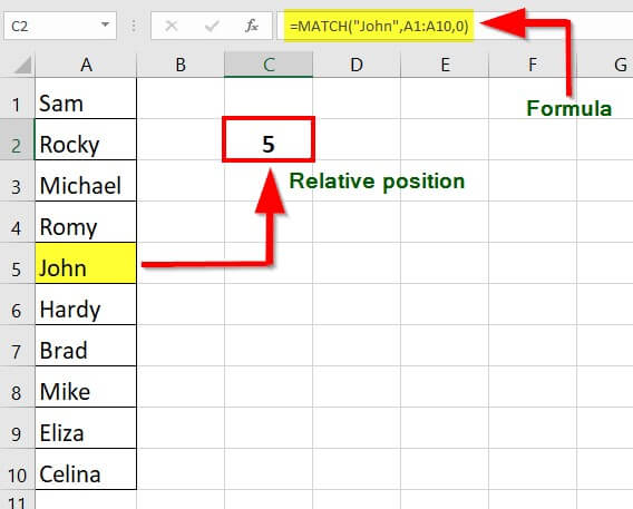
The utility of the MATCH function extends beyond simple searches within a range. For instance, one can use it in conjunction with other functions like INDEX and OFFSET to perform more complex operations.
Key Highlights
- The MATCH function in Excel can perform both exact and approximate matches.
- It can perform partial matches using wildcard operators such as * and ?.
- The MATCH function returns a #N/A error if it does not find a match in the given array.
- By using the MATCH and INDEX functions together, one can avoid using the VLOOKUP function to find a value at a matched position.
- The Match type is an optional argument in the MATCH function, and if not specified, it defaults to 1.
Syntax of MATCH Function in Excel
The syntax of MATCH function is as follows:
1. Lookup_value (required): Indicates the value whose position we want to find in the selected range. A lookup value can be text, number, logical value, or cell reference.
2. Lookup_array (required): The cell range that contains the lookup value. Lookup array can be a row or a column.
3. Match_Type (optional): An optional argument with values 1, 0, and -1. The match_type argument, set to 0, returns an exact match, while the other two values allow for an approximate match.
a) Match_Type “1”: If the match type value is set as 1, Excel provides a value less than or equal to the lookup value.
b) Match_Type “0”: If the match type value is set as 0, Excel provides the first value that is equal to the lookup value.
c) Match_Type “-1”: If the match type value is set as 0, Excel provides the smallest value that is greater than or equal to the lookup value.
Types of MATCH Function in Excel
You can download this MATCH Function Excel Template here – MATCH Function Excel Template
Here are the different types of MATCH functions in Excel:
#1 Exact MATCH
The MATCH function performs an exact match when the match type is set to zero. In the below-given example, the formula in E3 is:
=MATCH(E2,B3:B10,0)
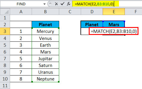
Here, the MATCH Function returns the Exact match as 4.
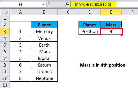
#2 Approximate MATCH
MATCH will perform an approximate match on values sorted A-Z when the match type is set to 1, finding the largest value less than or equal to the lookup value. In the below-given example, the formula in E3 is:
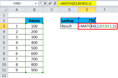
The MATCH in Excel returns an approximate match as 7.
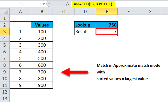
#3 Wildcard MATCH
MATCH function can perform a match using wildcards when the match type is set to zero. In the below-given example, the formula in E3 is:
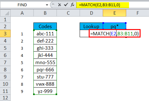
The MATCH function returns the result of wildcards as “pq”.
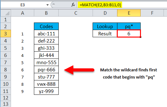
Points to Note:
- A MATCH Function is not case-sensitive.
- MATCH returns the #N/A error if there is no match is found.
- The argument lookup_array must be in descending order: True, False, Z-A,…9,8,7,6,5,4,3,…, and so on. However, if match_type is set to 1 or omitted, the lookup_array must be sorted in ascending order.
- The wildcard characters like an asterisk () and question mark (?) can be used in the lookup_value argument if match_type is set to 0 and lookup_value is in text format, regardless of whether the lookup_value contains these characters. The asterisk () matches any sequence of characters, while the question mark (?) matches any single character.
How to Use MATCH Function in Excel?
Example #1 Finding The Exact Match
The table below shows a list of ordered products with their order ID, unit price, and sales quantity. We want to find the position of “Deodorant” in the table using the MATCH function in Excel.
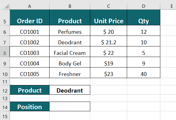
Solution:
Step 1: Select the cell where you want to display the position of the product “Deodorant“. In this case, let’s assume it is cell B12.
Step 2: Type the MATCH function in the formula bar: =MATCH(B12,B6:B10,0)
- The first argument in the formula is the lookup value, which is “Deodorant“, i.e., cell B12.
- The second argument of the MATCH function is the lookup array, which is the range B6:B10. This range contains the products listed in the table.
Note: The lookup_array can be a row or a column.
- The third argument of the MATCH function is the match type, which is 0. This means we want to find an exact match of the lookup value in the array.
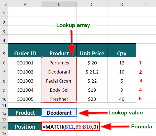
Step 3: Press Enter to get the result, as shown below.
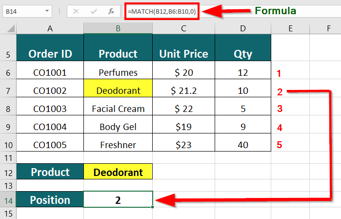
The formula returns the position of “Deodorant” in the table, which is 2. This means that “Deodorant” is the second product listed in the table.
Explanation of the Formula:
When you press the Enter key, Excel searches through the cells in the lookup array “B6:B10” to find an exact match for the lookup value “Deodorant”. After finding the match, it returns the position of the first cell containing the lookup value. In this scenario, the formula returns the value “2“, indicating that the first cell containing “Deodorant” is the second cell in the range B6:B10.
Example #2 Finding Partial MATCH using Wildcard Character
Let’s say we have a list of cities in Column A, and we want to find the position of the city that starts with “New” in the list.
Here’s how we can do it:
Step 1: Open a new Excel spreadsheet and enter the list of cities in Column A.
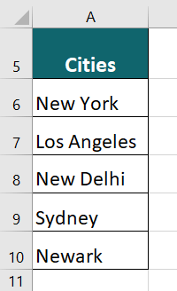
Step 2: In an empty cell, enter the formula =MATCH(“New*”,A6:A10,0).
Explanation of the Formula:
- “New*”: This is the search criteria. The asterisk () is a wildcard character representing any number of characters. So, “New” will match any city name that starts with “New”.
- A6:A10: This is the range of cells we want to search for our city name in.
- 0: This is the match_type argument. Here, we’re using an exact match, so we specify 0.
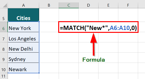
Step 3: Press the “Enter” key to display the result in the cell where you entered the formula.
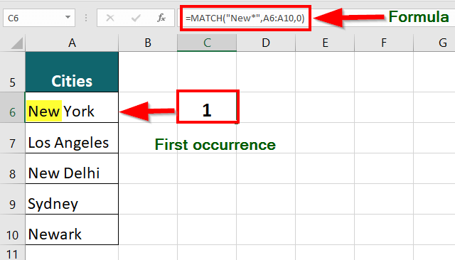
The result is “1,” which is the position of the first city that starts with “New”. In this case, “New York” is the first city that starts with “New” in the list.
Note: If multiple cities match the search criteria, the MATCH function will only return the position of the first occurrence.
Example #3 Using INDEX and MATCH Function Together
The table below shows a list of students with their marks in the subjects – Language, Maths, History, and Physics. Using the INDEX and MATCH functions together, we want to find Alex’s marks in History
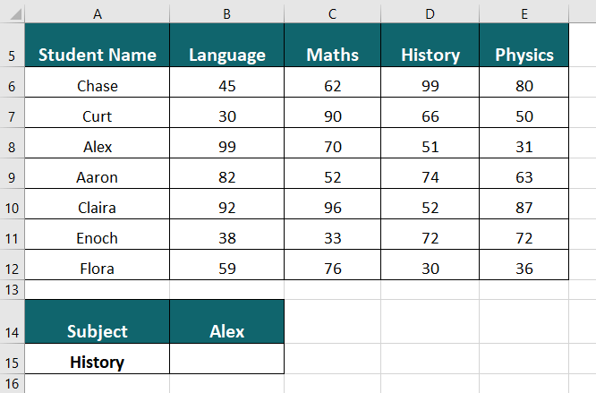
Solution:
Step 1: Select the cell where you want to display the result. In this case, it is cell B15.
Step 2: Enter the formula in the cell:
=INDEX(A5:E12,MATCH(B14,A5:A12,0),MATCH(A15,A5:E5,0))
- A5:E12: This is the range of cells containing the table of student data.
- B14: This is the value we want to find in the first column of the table, which is the name of the student whose marks we want to find (in this case, “Alex”).
- A5:A12: This is the range of cells containing the students’ names in the table’s first column.
- 0: This argument specifies that we want an exact match.
- A15: This is the value we’re looking for in row 5, which is the subject “History”.
- A5:E5: This is the cell range containing the subject names.
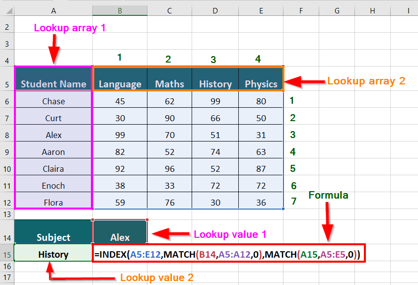
Step 3: Press Enter key to get the below result.
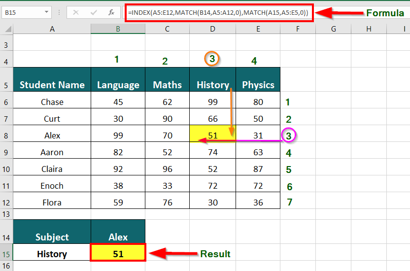
The INDEX and MATCH functions of Excel work together to provide the result of 51, which denote History marks of Alex.
Explanation of the Formula:
- The first MATCH function in the formula =INDEX(A5:E12,MATCH(B14,A5:A12,0),MATCH(A15,A5:E5,0)) searches for the student name “Alex” in the range A5:A12 and returns the relative position of that name within the range. The third argument of the MATCH function is 0, which specifies that we want an exact match. In this case, “Alex” is in the third row of the range, so the first MATCH function returns the value 3.
- The second MATCH function in the formula searches for the subject “History” in the range A5:E5 and returns the relative position of that subject within the range. Again, the third argument of the MATCH function is 0, which specifies that we want an exact match. In this case, “History” is in the third column of the range, so the second MATCH function returns the value 3.
- The INDEX function then uses these two values (3 and 3) to return the corresponding value in the table, which is the marks that Alex scored in History (51).
Example #4 When a Cell contains One of Many Things
Generic formula: {=INDEX(results,MATCH(TRUE,ISNUMBER(SEARCH(things,A1)),0))}
Explanation: The INDEX / MATCH function formed on the SEARCH function can be used to check a cell for one of many things and give back a custom result for the first match found.
In the example shown below, the formula in cell C5 is:
{=INDEX(results,MATCH(TRUE,ISNUMBER(SEARCH(things,B5)),0))}
Since the above is an array formula, it should be entered using Control + Shift + Enter keys.
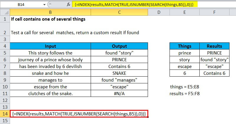
Explanation of the Formula:
- This formula uses two named ranges: E5:E8 is named “things”, and F5:F8 is named “results”.
- Ensure using the name ranges with the same names (depending on the data). If one doesn’t want to use named ranges, use absolute references instead.
- The main part of this formula is the below snippet:
ISNUMBER(SEARCH(things, B5)
- This is based on another formula that checks a cell for a single substring. If the cell has the substring, the formula gives TRUE; if not, the formula gives FALSE
Example #5 Lookup using the Lowest Value
Generic formula =INDEX(range,MATCH(MIN(vals),vals,0))
Explanation: To lookup information associated with the lowest value in a table, one can use a formula depending on MATCH, INDEX, and MIN functions.
In the below example, a formula is used to find the name of the contractor who has the lowest bid. The formula in F6 is:
=INDEX(B5:B9,MATCH(MIN(C5:C9),C5:C9,0)))
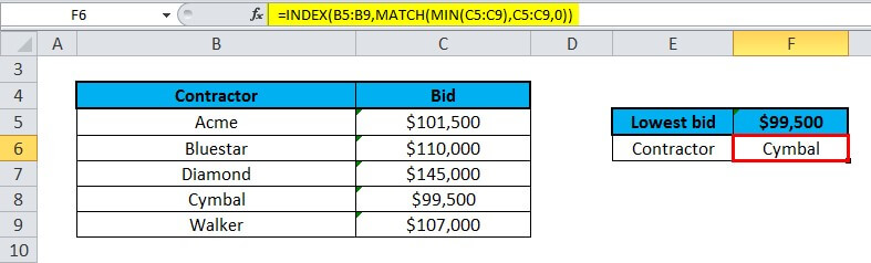
Explanation of the Formula:
- Working from the inside out, the MIN function is generally used to find the lowest bid in the range C5:C9:
- The result, 99500, is fed into the MATCH function as the lookup value:
- MATCH then gives back the position of this value in the range, 4, which goes into INDEX as the row number and B5:B9 as the array:
=INDEX(B5:B9, 4) // returns Cymbal
- The INDEX function then gives back the value at that position: Cymbal.
Match Function Errors
If you get an error from the Match function, this is likely to be the #N/A error:
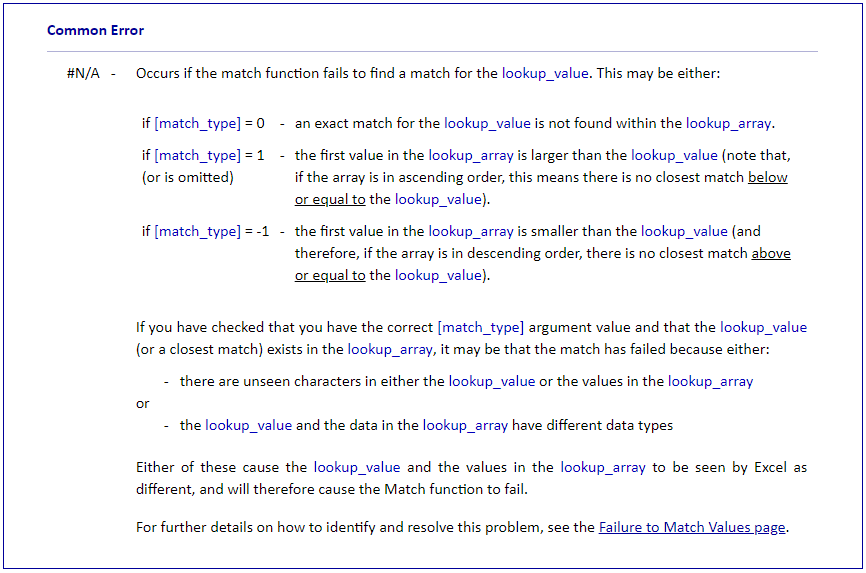
Also, some users experience the following common problem with the Match Function:
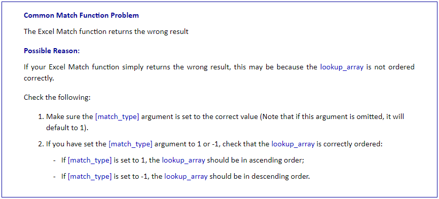
Things to Remember
- MATCH types: One can use three match types with the MATCH function: 0, 1, and -1. The default match type is 0, which finds an exact match. Match type 1 finds the largest value that is less than or equal to the lookup_value, while match type -1 finds the smallest value that is greater than or equal to the lookup_value.
- Array size: The lookup_array argument must be a one-dimensional array or a reference to a one-dimensional range of cells. If the lookup_array is not one-dimensional, the MATCH function will return a #N/A error.
- Sorted order: If the values in the lookup_array are not sorted in ascending order, the MATCH function in Excel may return an incorrect result. In such cases, use the match_type argument to specify the appropriate match type.
- Exact MATCH: If the MATCH function does not find the lookup_value in the lookup_array, it will return a #N/A error. You can use the IFERROR function to handle this error and return a more meaningful result.
- Relative or absolute cell reference: The MATCH function is compatible with both relative and absolute cell references. When copying the formula to other cells, the function will adjust the cell references accordingly.
Frequently Asked Questions (FAQs)
Q1. What is an example of a MATCH function in Excel?
Answer: The MATCH function searches for a given value in a data set and provides the position of that value in the range. For instance, suppose you have a data set that includes items like Spinach, Brinjal, Tomato, French Bean, and Cabbage in the range B6:B10. If you want to find the position of the value “French Bean” in the range, you can use the MATCH function.
The formula =MATCH(B12,B6:B10,0) returns the “French Bean” position in the range B6:B10 as the number 4.
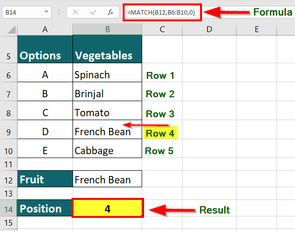
Q2. What is the benefit of including the MATCH function within an INDEX function?
Answer: Including the MATCH function within an INDEX function allows you to retrieve data dynamically based on specific search criteria.
Suppose you have a list of fruits and their prices in a table. You want to retrieve the price of a specific fruit, say “Apple”, from the table. One way to do this is to search the table for the row containing “Apple” manually, and then look for the price in the corresponding column. However, if you have a large dataset with many rows and columns, this can be a time-consuming and error-prone process. Instead, you can use the MATCH function to find the row number of “Apple” in the table and then use the INDEX function to retrieve the price from the corresponding column. The formula would look like this:
=INDEX(B2:E6,MATCH(“Apple”,A2:A6,0),3)
The MATCH function searches for “Apple” in the table’s first column (A2:A6) and returns the row number where it is found. The INDEX function then retrieves the value from the table’s third column (price column) at the intersection of the row and column numbers that the MATCH function returns.
Q3. Can the MATCH function have multiple criteria?
Answer: It is possible to use the MATCH function with multiple criteria by combining it with other functions such as INDEX, SUMPRODUCT, and COUNTIFS. For instance, consider this formula:
= MATCH(1, (B2:B10=”Sales”) * (C2:C10>20000), 0) + COUNTIFS(B2:B10, “Sales”, C2:C10, “>20000”)
This formula uses MATCH with multiple criteria to find the position of the first employee in the “Sales” department who earns more than $20,000 per year. Then, it adds the count of cells that satisfy only the second condition using the COUNTIFS function.
Q4. What is the difference between MATCH and VLOOKUP in Excel?
Answer: The MATCH function helps us find the location of a particular value in a column or row, while the VLOOKUP function helps us retrieve information associated with that value.
For instance, if we want to find the price of oranges in the following table, we will have to use the MATCH function in conjunction with the INDEX function to find the price. Alternatively, the VLOOKUP function can directly provide the price of oranges at $0.75.
|
Product |
Price |
| Apples | $1.00 |
| Oranges | $0.75 |
| Bananas | $0.50 |
The formula for using MATCH and INDEX functions together is =INDEX(B:B, MATCH(“Oranges”, A:A, 0)). Using MATCH, this formula finds the position of “Oranges” in column A, which returns the value 2. Then, INDEX retrieves the value in column B’s corresponding row, i.e., $0.75.
- The VLOOKUP function formula is =VLOOKUP(“Oranges”, A:B, 2, 0). This formula looks for “Oranges” in the first column of the range A:B, and returns the corresponding value from the second column (i.e., the price column), resulting in $0.75.
Recommended Articles
The above article is our guide to using the MATCH function in Excel. Here are some further examples of expanding understanding:
- Excel Match Multiple Criteria
- How to Match Data in Excel
- Matching Columns in Excel
- Compare Two Columns in Excel for Matches