Finding empty cells excel

See all How-To Articles

In this tutorial, you will learn how to find blank cells in Excel and Google Sheets.

Find & Select Empty Cells

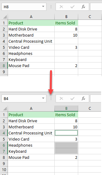
There is an easy way to select all the blank cells in any selected range in Excel. Although this method won’t show you the number of blank cells, it will highlight all of them so you can easily locate them in a spreadsheet.

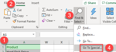
1. First, select the entire data range. Then in the Ribbon, go to Home > Find & Select > Go To Special.

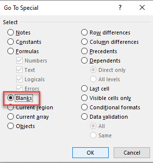
2. In Go To Special dialog window click on Blanks and when done press OK.

As a result, all blank cells are selected.

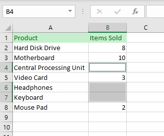
With this method, you won’t find pseudo-blank cells (cells with formulas that return blanks and cells containing only spaces).

Other ways to identify blanks:

• IsEmpty Function in VBA
• How to use the ISBLANK Function

Find Blank Cells in Google Sheets

Unlike Excel, Google Sheets doesn’t have a Go To Special feature. But you can identify blank cells and select them one-by-one, highlight them, or replace them.

Sometimes you need to check if a cell is blank, generally because you might not want a formula to display a result without input.

In this case we’re using IF with the ISBLANK function:

• =IF(ISBLANK(D2),»Blank»,»Not Blank»)

Which says IF(D2 is blank, then return «Blank», otherwise return «Not Blank»). You could just as easily use your own formula for the «Not Blank» condition as well. In the next example we’re using «» instead of ISBLANK. The «» essentially means «nothing».

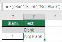
=IF(D3=»»,»Blank»,»Not Blank»)

This formula says IF(D3 is nothing, then return «Blank», otherwise «Not Blank»). Here is an example of a very common method of using «» to prevent a formula from calculating if a dependent cell is blank:

• =IF(D3=»»,»»,YourFormula())

  IF(D3 is nothing, then return nothing, otherwise calculate your formula).

In Excel, a blank cell doesn’t always mean a cell with an empty string («»). An example to this is invisible characters like a new line character which can be entered by pressing the Alt + Enter key combination when you’re in a cell. You can detect the cells that are actually blank by using Excel’s Go To feature. In this article, we’re going to show you how to find blank cells in Excel using the Go To feature.

How to Find Blank Cells in Excel using Go To

1. Begin by selecting your data including the blank rows
2. Open the Go To Special dialog by following HOME > Find & Select > Go To Special in the ribbon
3. Select the Blanks option
4. Click OK to apply your selection

In our example, you can see that Excel selects only two cells, D6 and C7, even though the cells F6 and F7 look empty as well. This is not an error, but an example of «actually not blank cells». The cells like F6 and F7 will also affect results of the COUNTA function, which also counts these types of cells. For example, the =COUNTA(B3:F8) formula returns 28 as it ignores only cells D6 and C7.

You might want to be extra careful when removing blank rows using the Go To feature, because it selects individual blank cells in rows that have values. Removing them will cause data loss, even though you can revert your actions with Undo.

Some blank cells in a worksheet are actually not empty. But their existence will make you confused. Therefore, you need to find those non-empty cells in your Excel worksheet.

There are many conditions that a cell will be non-empty while the content in it is invisible. For example, a formula will return null value, the font color in the cell is the same as the fill color, or the invisible values that returned by VBA macros. All those reasons can make the content invisible. But actually those cells are non-empty. And to avoid the problems caused by those cells in your work, you can use the following 4 methods to find those cells that contain invisible contents.

Method 1: Use Ctrl and Arrows Keys

In this method, you need to use the Ctrl and Arrows keys in the keyboard. And below we will demonstrate the thorough step.

In the image below, there is a blank row in the range.

And before deleting the row, you need to make sure that there are no contents in the row. Otherwise some errors will appear and can result in mistakes in other cells.

1. Click the cell A1 in the worksheet.
2. And then press the shortcut keys “Ctrl + ↓” on the keyboard. When you use this shortcut keys combo, the cursor will move to the last non-empty cell in the column.

And in this example, it will move to cell A7. When you press the keys again, the cursor will move to the first non-empty cell in the next range. And in this example, it will move to cell A9. This means that cell A8 is really an empty cell.

1. Now you need to check the second column. Here click the cell B1.
2. And then press the shortcut keys “Ctrl + ↓” again.
3. After that, see where the cursor position at.

This time, the cursor move to cell B14 directly. This means that cell B8 is a non-empty cell.

1. Now click the cell B8 and check the value in it. In the formula bar, you can see that there is a formula in the cell.

Here because the font color of the cell is white, so you cannot see it.

1. Now continue using the shortcut keys and check the next column.

When you need to check many cells in a range, clicking those cells one after another and check in the formula bar can be time-consuming. Therefore, you can use this method. Besides, you can also combine other arrow keys with the Ctrl key to check other rows or columns.

Method 2: Use ISBLANK Function

Instead of using shortcut keys, you can also use the ISBLANK function in your worksheet.

1. Click a blank cell in the worksheet. In this example, we click cell D8.
2. And then input the formula into the cell.

=ISBLANK(A8)

1. Next press the button “Enter” on the keyboard. Thus, you will get a result in this cell.

Here the formula returns a result “TRUE” in the cell.

1. Now click the fill handle of the cell and drag rightward to fill other cells.

And then you will see all the result for the three cells. You can see that the result in cell E8 is “FALSE”, which means that cell B8 is a non-empty cell.

You can see that using this function is very easy. When you need to check for a whole column or a whole row, you can use this method quickly.

Method 3: Use Conditional Formatting

In this method, you can also use conditional formatting to highlight certain cells. Here you can highlight the empty cells in a range.

1. Select the target range that contains all the target cells.
2. And then click the button “Conditional Formatting”.
3. After that, in the drop-down menu, choose the option “New Rule”.
4. In the “New Formatting Rule” window, choose the last option that needs to use formula.
5. Now input the formula into the text box:

=ISBLANK(A1)

Here you will also use the ISBLANK function. Here make sure that the cell is the first cell in the range. On the other hand, if you need to highlight non-empty cells in a range, you can input this formula:

=NOT(ISBLANK(A6))

1. And then click the button “Format”.
2. In the “Format Cells” window, set a format for the cell.
3. When you have finished the setting, click the button “OK”.
4. Next click “OK” in the “New Formatting Rule” window.

And then you can see that in the range, true empty cells will be highlighted.

Hence you can know that the cell B8 contains a value. Using conditional formatting can also help you judge those cells quickly.

Method 4: Use VBA Macro

This is the last method and you will use the VBA macros.

1. Press the shortcut keys “Alt +F11” on the keyboard to open the VBA editor.
2. And then click the button “Insert” in the toolbar.
3. After that, choose the option “Module” in the sub menu. Thus, you have inserted a new module into the file.
4. Now copy and paste the following codes into the module.

Sub findcell()

    Dim cel As Range

    For Each cel In Range(“A1:C14”)

        If IsEmpty(cel) = True Then

            cel.Interior.Color = vbYellow

        End If

    Next cel

End Sub

Here we will also find the empty cells and format them. If you need to format cells that contain contents, you can also modify the codes according to your need. You may also pay attention that you need to clear all the conditional formatting. Otherwise the format of VBA macro will be covered by the format of conditional formatting. And this will cause trouble to you.

1. Now click the button “Run Sub” in the toolbar or press the button “F5” on the keyboard to run this macro.
2. After that, come back to the worksheet. And you will see the result like the image below shows.

The formats of real empty cells change. Therefore, cell B8 is a non-empty cell in this range.

A Comparison between the Methods

Here we have listed the advantages and disadvantages of the above four methods.

Comparison	Ctrl and Arrows Keys	ISBLANK Function	Conditional Formatting	VBA Macro
Advantages	You can apply this method quickly when you need to find non-empty cells in a row or a column.	When you need to judge cells in a range, this function is very helpful.	All the result can be listed clearly in the worksheet. And you can choose to format empty cells or non-empty cells according to your need.	With just one click, you can easily get the result. Besides, you can also modify the codes according to your need.
Disadvantages	Compared with other methods, this method will be time-consuming.	If the non-empty cells are separate in different position, it will be inconvenient to use this formula.	The format of conditional formatting will interfere with other cell formats.	If you are not familiar with Excel VBA, the task will be more complicated.

From the above analysis, you will have a comprehensive understanding of the four methods. And you can choose the most suitable method according to your need.

Protect Your Excel Files

The safety of mission-critical Excel files in your storage devices is very essential. Therefore, you need to carefully protect your Excel files. The Excel files have long been victim to malicious virus and malware. Whenever you find Excel corruption in your computer, you need to take the right actions. And you can also use a recovery tool to repair Excel file. In all the methods that can deal with Excel errors, using a tool is the most cost-effective method.

Author Introduction:

Anna Ma is a data recovery expert in DataNumen, Inc., which is the world leader in data recovery technologies, including repair docx data problem and outlook repair software products. For more information visit www.datanumen.com

Author: Oscar Cronquist Article last updated on February 02, 2023

This article demonstrates how to find empty cells and populate them automatically with a formula that adds numbers above and returns a total.

Is it possible to quickly select all empty cells and then sum cells above to the next empty cell? Yes, I will show you how.

Can I have a formula in grand total (row 18) that only sums all the totals above? Yes!

1. How to select empty cells in a cell range

The image above demonstrates how to find empty cells in a given cell range.

1. Select all values and the blank total cells.
   
2. Press F5, a dialog box appears.
   
3. Press the left mouse on the «Special…» button.
   
4. Press on «Blanks» to select it, then press on the «OK» button.

Back to top

2. Populate empty cells with a formula

1. Go to tab «Home» on the ribbon and press with left mouse button on the «AutoSum» button.
   
2. All empty cells now have a SUM formula that adds all the above values to the next SUM formula.
   

3. Add grand totals that only sums cells populated with formulas

1. Select cell C18 and type this formula:

   =SUMPRODUCT(ISFORMULA(C3:C17)*C3:C17)

   

2. Press Enter. Copy cell C18 and paste to cell range D18:F18.
   

3.1 Explaining formula in cell C18

Step 1 — Check if cell contains a formula

The ISFORMULA function checks if a cell in cell range C3:C17 has a formula. It returns TRUE or FALSE.

ISFORMULA(C3:C17)

returns this array:

{FALSE; FALSE; TRUE; FALSE; FALSE; FALSE; TRUE; FALSE; FALSE; TRUE; FALSE; FALSE; FALSE; FALSE; TRUE}

The picture below shows this array in column D.

The array shows that there is a formula in C5, C9, C12, and C17.

Step 2 —  Multiply with value

The asterisk character allows you to multiply numbers and boolean values.

ISFORMULA(C3:C17)*C3:C17 multiplies the boolean values with their corresponding values in column C, shown in column E below.

ISFORMULA(C3:C17)*C3:C17

becomes

{FALSE; FALSE; TRUE; FALSE; FALSE; FALSE; TRUE; FALSE; FALSE; TRUE; FALSE; FALSE; FALSE; FALSE; TRUE}*C3:C17

becomes

{FALSE; FALSE; TRUE; FALSE; FALSE; FALSE; TRUE; FALSE; FALSE; TRUE; FALSE; FALSE; FALSE; FALSE; TRUE}*{748; 508; 1256; 283; 960; 23; 1266; 821; 658; 1479; 970; 109; 599; 252; 1930}

and returns

{0; 0; 1256; 0; 0; 0; 1266; 0; 0; 1479; 0; 0; 0; 0; 1930}

Step 3 — Add values and return the total

The SUMPRODUCT function then sums all values in the array.

SUMPRODUCT(ISFORMULA(C3:C17)*C3:C17)

becomes

SUMPRODUCT({0; 0; 1256; 0; 0; 0; 1266; 0; 0; 1479; 0; 0; 0; 0; 1930})

and returns 5931 in cell C18.

Why not use the SUM function? You need to enter it as an array formula if you use the SUM function. Use the SUM function if you are an Excel 365 user.

Back to top

4. Add grand totals that only sums cells populated with formulas — Excel 2013

The following formula won’t work, the SUMIF function seems to not be capable of processing the ISFORMULA function. The ISFORMULA function is an Excel 2013 function, they seem incompatible.

=SUMIF(C3:C17, ISFORMULA(C3:C17))

Let me know if you have a solution that allows me to use the SUMIF function.

5. Add grand totals that only sums cells populated with formulas — Excel 365

=SUM(FILTER(C3:C17, ISFORMULA(C3:C17)))

5.1 Explaining formula

Step 1 — Check if cell contains formula

The ISFORMULA function returns a boolean value TRUE or FALSE if a cell contains a formula or not.

ISFORMULA(C3:C17)

Step 2 — Filter numbers based on boolean values

FILTER(C3:C17,ISFORMULA(C3:C17))

Step 3 — Add numbers and return a total

SUM(FILTER(C3:C17,ISFORMULA(C3:C17)))

Running totals based on criteria
Andrew asks: LOVE this example, my issue/need is, I need to add the results. So instead of States and Names, […]

Sum unique numbers
Table of Contents Sum unique numbers Get Excel *.xlsx file Sum unique distinct numbers Get Excel *.xlsx file Sum number […]

Sum cells based on criteria
Katie asks: I have 57 sheets many of which are linked together by formulas, I need to get numbers from […]

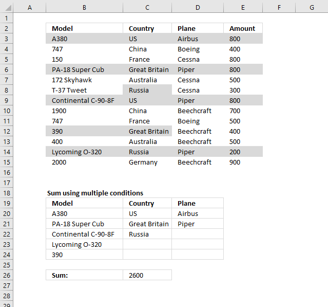
Sum based on OR – AND logic
Question: It’s easy to sum a list by multiple criteria, you just use array formula a la: =SUM((column_plane=TRUE)*(column_countries=»USA»)*(column_producer=»Boeing»)*(column_to_sum)) But all […]

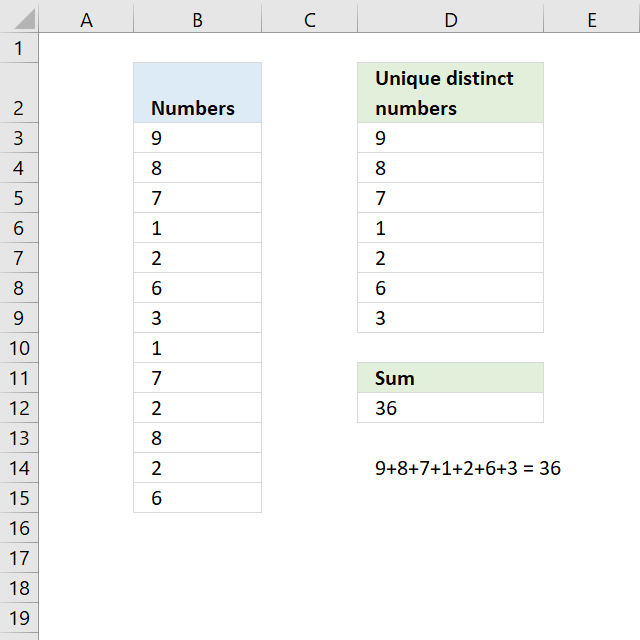
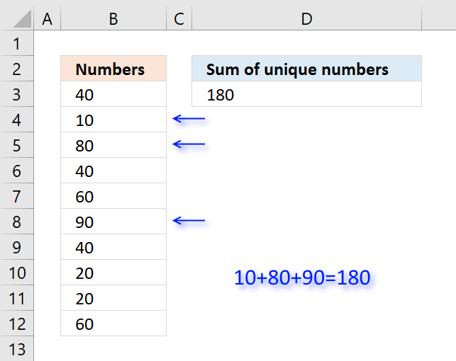
Sum unique distinct numbers
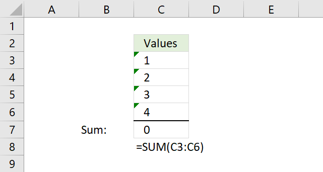
The image above shows numbers in column B, some of these numbers are duplicates. The formula in D12 adds unique […]

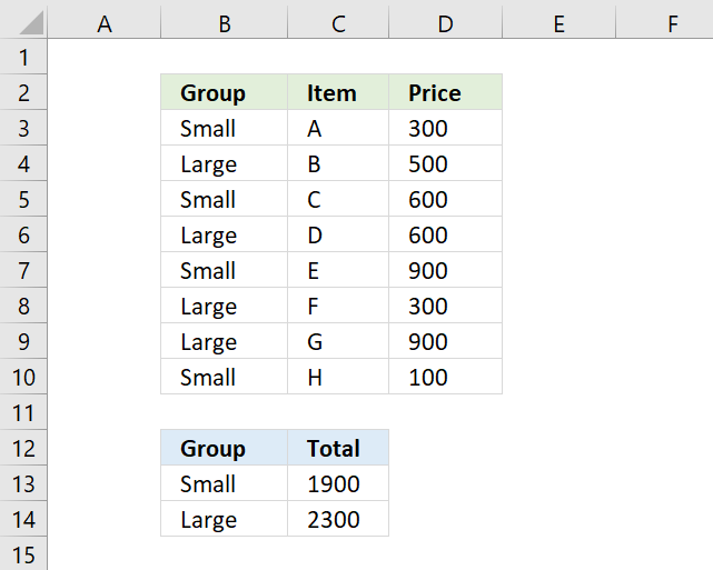
Sum by group
To extract groups from cell range B3:B10 I use the following regular formula in cell B13.

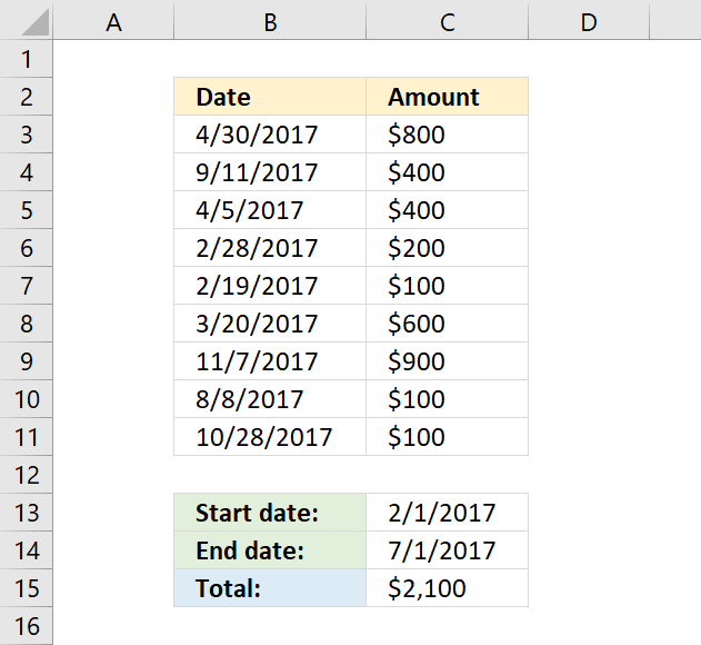
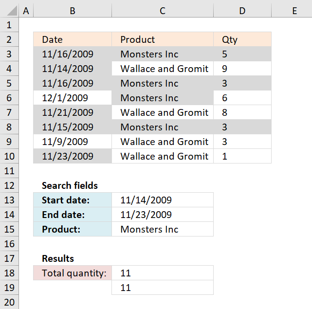
Sum numbers between two dates
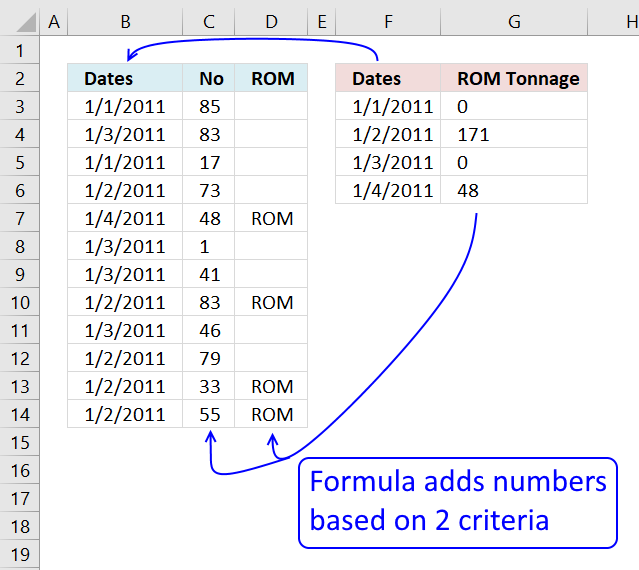
The formula in cell C15 uses two dates two to filter and then sum values in column C, the SUMIFS […]

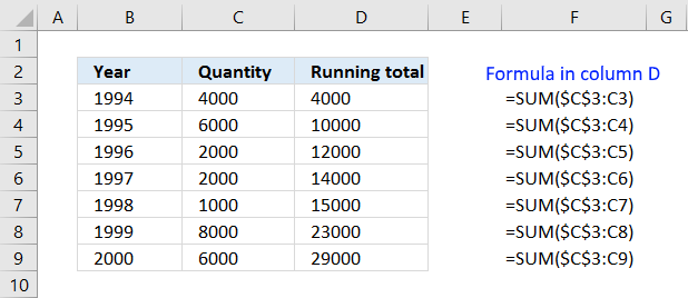
How to create running totals
This article demonstrates a formula that calculates a running total. A running total is a sum that adds new numbers […]

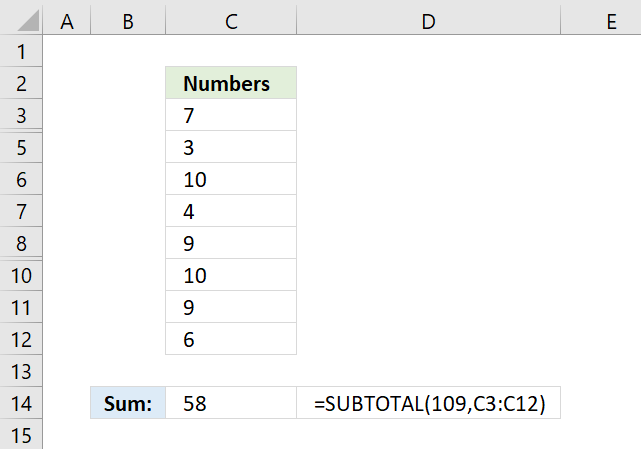
Sum only visible cells
The SUBTOTAL function lets you sum values in a cell range that have some rows hidden or filtered, the picture […]

How to sum a cell range
I will in this article demonstrate different ways to sum values, the first method is so easy and fast it’s […]

Excel formula not working
This article explains why your formula is not working properly, there are usually four different things that can go wrong. […]

Latest updated articles.

More than 300 Excel functions with detailed information including syntax, arguments, return values, and examples for most of the functions used in Excel formulas.

More than 1300 formulas organized in subcategories.

Excel Tables simplifies your work with data, adding or removing data, filtering, totals, sorting, enhance readability using cell formatting, cell references, formulas, and more.

Allows you to filter data based on selected value , a given text, or other criteria. It also lets you filter existing data or move filtered values to a new location.

Lets you control what a user can type into a cell. It allows you to specifiy conditions and show a custom message if entered data is not valid.

Lets the user work more efficiently by showing a list that the user can select a value from. This lets you control what is shown in the list and is faster than typing into a cell.

Lets you name one or more cells, this makes it easier to find cells using the Name box, read and understand formulas containing names instead of cell references.

The Excel Solver is a free add-in that uses objective cells, constraints based on formulas on a worksheet to perform what-if analysis and other decision problems like permutations and combinations.

An Excel feature that lets you visualize data in a graph.

Format cells or cell values based a condition or criteria, there a multiple built-in Conditional Formatting tools you can use or use a custom-made conditional formatting formula.

Lets you quickly summarize vast amounts of data in a very user-friendly way. This powerful Excel feature lets you then analyze, organize and categorize important data efficiently.

VBA stands for Visual Basic for Applications and is a computer programming language developed by Microsoft, it allows you to automate time-consuming tasks and create custom functions.

A program or subroutine built in VBA that anyone can create. Use the macro-recorder to quickly create your own VBA macros.

UDF stands for User Defined Functions and is custom built functions anyone can create.

A list of all published articles.

In this article, we will learn:

How To Check If A Cell Is Blank Using IF

How To Check If A Cell Is Blank Using ISBLANK

Count Blank Cells Using COUNTIF

Count Blank Cells Using COUNTBLANK

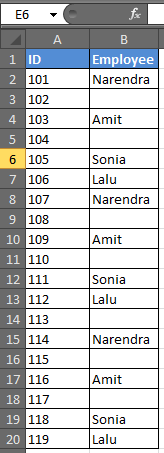
Assume you have this data.

Let’s just step into the example.

How To Check If A Cell Is Blank Using IF

Generic Formula

=IF(cell_address=»»,TRUE,FALSE)

In the above data, there are some names that are missing. In Column C you want TRUE if it doesn’t have a name and FALSE if it does. It is easy to do this. In C2 write this formula and copy it in the cells below.

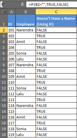
The formula simply checks to see if the cell is blank or not. It uses “”  to indicate blank. Prints TRUE  if it is blank, and FALSE if not.

How To Check If A Cell Is Blank Using ISBLANK

Generic Formula

Now the same task can be done easily by using the ISBLANKfunction in excel 2016.

ISBLANK takes only one argument and that is the cell you want to check.

In D2 write this formula and copy it below cells.

This will be your result.

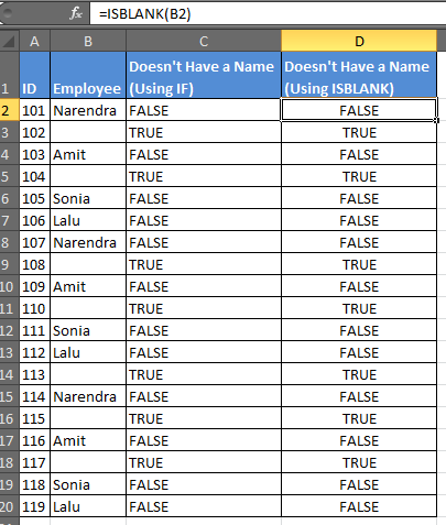
You got the same answers by giving just one argument in ISBLANK.

Mostly you would want to do something after knowing if the cell is blank or not. This is where IF is necessary.

For example, if you want to print the name Cells of B column has one, and “mystry_man” if it is a blank cell. You can use IF and ISBLANK in excel together.

In Range E2, write this formula:

Count Blank Cells Using COUNTIF

Generic Formula

Now if you want to know how many blank cells there are, you can use this formula.

In any version of Excel 2016, 2013, 2010, write this formula in any cell.

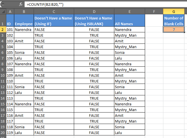
We have our answer as 7 for this example.

Now if you want to know how many names there are, you need to count if not blank. Use the COUNTA function to count non-blank cells in a range.

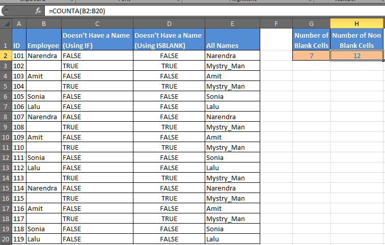
Count Blank Cells Using COUNTBLANK

Generic Formula

COUNTA counts if cell contains any text and the COUNTBLANK function counts all blank cells in a range in Excel. It only requires one argument to count empty cells in a range.

In cell G2, enter this formula:

COUNTBLANK will find blank cells in excel of the given range.

We learned how to work with blank cells in excel, how to find blank cells, how to count blank cells in a range, how to check if a cell is empty or not, how to manipulate blank cells etc.

Related Articles:

How to Calculate Only If Cell is Not Blank in Excel

Adjusting a Formula to Return a Blank

Checking Whether Cells in a Range are Blank, and Counting the Blank Cells

SUMIF with non-blank cells

Only Return Results from Non-Blank Cells

Popular Articles:

50 Excel Shortcuts to Increase Your Productivity

How to use the VLOOKUP Function in Excel

How to use the COUNTIF function in Excel

How to use the SUMIF Function in Excel