

Use the Find and Replace features in Excel to search for something in your workbook, such as a particular number or text string. You can either locate the search item for reference, or you can replace it with something else. You can include wildcard characters such as question marks, tildes, and asterisks, or numbers in your search terms. You can search by rows and columns, search within comments or values, and search within worksheets or entire workbooks.

Find
To find something, press Ctrl+F, or go to Home > Editing > Find & Select > Find.
Note: In the following example, we’ve clicked the Options >> button to show the entire Find dialog. By default, it will display with Options hidden.

-
In the Find what: box, type the text or numbers you want to find, or click the arrow in the Find what: box, and then select a recent search item from the list.
Tips: You can use wildcard characters — question mark (?), asterisk (*), tilde (~) — in your search criteria.
-
Use the question mark (?) to find any single character — for example, s?t finds «sat» and «set».
-
Use the asterisk (*) to find any number of characters — for example, s*d finds «sad» and «started».
-
Use the tilde (~) followed by ?, *, or ~ to find question marks, asterisks, or other tilde characters — for example, fy91~? finds «fy91?».
-
-
Click Find All or Find Next to run your search.
Tip: When you click Find All, every occurrence of the criteria that you are searching for will be listed, and clicking a specific occurrence in the list will select its cell. You can sort the results of a Find All search by clicking a column heading.
-
Click Options>> to further define your search if needed:
-
Within: To search for data in a worksheet or in an entire workbook, select Sheet or Workbook.
-
Search: You can choose to search either By Rows (default), or By Columns.
-
Look in: To search for data with specific details, in the box, click Formulas, Values, Notes, or Comments.
Note: Formulas, Values, Notes and Comments are only available on the Find tab; only Formulas are available on the Replace tab.
-
Match case — Check this if you want to search for case-sensitive data.
-
Match entire cell contents — Check this if you want to search for cells that contain just the characters that you typed in the Find what: box.
-
-
If you want to search for text or numbers with specific formatting, click Format, and then make your selections in the Find Format dialog box.
Tip: If you want to find cells that just match a specific format, you can delete any criteria in the Find what box, and then select a specific cell format as an example. Click the arrow next to Format, click Choose Format From Cell, and then click the cell that has the formatting that you want to search for.
Replace
To replace text or numbers, press Ctrl+H, or go to Home > Editing > Find & Select > Replace.
Note: In the following example, we’ve clicked the Options >> button to show the entire Find dialog. By default, it will display with Options hidden.

-
In the Find what: box, type the text or numbers you want to find, or click the arrow in the Find what: box, and then select a recent search item from the list.
Tips: You can use wildcard characters — question mark (?), asterisk (*), tilde (~) — in your search criteria.
-
Use the question mark (?) to find any single character — for example, s?t finds «sat» and «set».
-
Use the asterisk (*) to find any number of characters — for example, s*d finds «sad» and «started».
-
Use the tilde (~) followed by ?, *, or ~ to find question marks, asterisks, or other tilde characters — for example, fy91~? finds «fy91?».
-
-
In the Replace with: box, enter the text or numbers you want to use to replace the search text.
-
Click Replace All or Replace.
Tip: When you click Replace All, every occurrence of the criteria that you are searching for will be replaced, while Replace will update one occurrence at a time.
-
Click Options>> to further define your search if needed:
-
Within: To search for data in a worksheet or in an entire workbook, select Sheet or Workbook.
-
Search: You can choose to search either By Rows (default), or By Columns.
-
Look in: To search for data with specific details, in the box, click Formulas, Values, Notes, or Comments.
Note: Formulas, Values, Notes and Comments are only available on the Find tab; only Formulas are available on the Replace tab.
-
Match case — Check this if you want to search for case-sensitive data.
-
Match entire cell contents — Check this if you want to search for cells that contain just the characters that you typed in the Find what: box.
-
-
If you want to search for text or numbers with specific formatting, click Format, and then make your selections in the Find Format dialog box.
Tip: If you want to find cells that just match a specific format, you can delete any criteria in the Find what box, and then select a specific cell format as an example. Click the arrow next to Format, click Choose Format From Cell, and then click the cell that has the formatting that you want to search for.
There are two distinct methods for finding or replacing text or numbers on the Mac. The first is to use the Find & Replace dialog. The second is to use the Search bar in the ribbon.
Find & Replace dialog
Search bar and options

-
Press Ctrl+F or go to Home > Find & Select > Find.
-
In Find what: type the text or numbers you want to find.
-
Select Find Next to run your search.
-
You can further define your search:
-
Within: To search for data in a worksheet or in an entire workbook, select Sheet or Workbook.
-
Search: You can choose to search either By Rows (default), or By Columns.
-
Look in: To search for data with specific details, in the box, click Formulas, Values, Notes, or Comments.
-
Match case — Check this if you want to search for case-sensitive data.
-
Match entire cell contents — Check this if you want to search for cells that contain just the characters that you typed in the Find what: box.
-
Tips: You can use wildcard characters — question mark (?), asterisk (*), tilde (~) — in your search criteria.
-
Use the question mark (?) to find any single character — for example, s?t finds «sat» and «set».
-
Use the asterisk (*) to find any number of characters — for example, s*d finds «sad» and «started».
-
Use the tilde (~) followed by ?, *, or ~ to find question marks, asterisks, or other tilde characters — for example, fy91~? finds «fy91?».

-
Press Ctrl+F or go to Home > Find & Select > Find.
-
In Find what: type the text or numbers you want to find.
-
Select Find All to run your search for all occurrences.

Note: The dialog box expands to show a list of all the cells that contain the search term, and the total number of cells in which it appears.
-
Select any item in the list to highlight the corresponding cell in your worksheet.
Note: You can edit the contents of the highlighted cell.

-
Press Ctrl+H or go to Home > Find & Select > Replace.
-
In Find what, type the text or numbers you want to find.
-
You can further define your search:
-
Within: To search for data in a worksheet or in an entire workbook, select Sheet or Workbook.
-
Search: You can choose to search either By Rows (default), or By Columns.
-
Match case — Check this if you want to search for case-sensitive data.
-
Match entire cell contents — Check this if you want to search for cells that contain just the characters that you typed in the Find what: box.
Tips: You can use wildcard characters — question mark (?), asterisk (*), tilde (~) — in your search criteria.
-
Use the question mark (?) to find any single character — for example, s?t finds «sat» and «set».
-
Use the asterisk (*) to find any number of characters — for example, s*d finds «sad» and «started».
-
Use the tilde (~) followed by ?, *, or ~ to find question marks, asterisks, or other tilde characters — for example, fy91~? finds «fy91?».
-
-
-
In the Replace with box, enter the text or numbers you want to use to replace the search text.
-
Select Replace or Replace All.
Tips:
-
When you select Replace All, every occurrence of the criteria that you are searching for is replaced.
-
When you select Replace, you can replace one instance at a time by selecting Next to highlight the next instance.
-
-
Select any cell to search the entire sheet or select a specific range of cells to search.
-
Press Command + F or select the magnifying glass to expand the Search bar and type the text or number you want to find in the search field.
Tips: You can use wildcard characters — question mark (?), asterisk (*), tilde (~) — in your search criteria.
-
Use the question mark (?) to find any single character — for example, s?t finds «sat» and «set».
-
Use the asterisk (*) to find any number of characters — for example, s*d finds «sad» and «started».
-
Use the tilde (~) followed by ?, *, or ~ to find question marks, asterisks, or other tilde characters — for example, fy91~? finds «fy91?».
-
-
Press return.
Notes:
-
To find the next instance of the item you are searching for, press return again or use the Find dialog box and select Find Next.
-
To specify additional search options, select the magnifying glass and select Search in Sheet or Search in Workbook. You can also select the Advanced option, which launches the Find dialog.
Tip: You can cancel a search in progress by pressing ESC.
-
Find
To find something, press Ctrl+F, or go to Home > Editing > Find & Select > Find.
Note: In the following example, we’ve clicked > Search Options to show the entire Find dialog. By default, it will display with Search Options hidden.

-
In the Find what: box, type the text or numbers you want to find.
Tips: You can use wildcard characters — question mark (?), asterisk (*), tilde (~) — in your search criteria.
-
Use the question mark (?) to find any single character — for example, s?t finds «sat» and «set».
-
Use the asterisk (*) to find any number of characters — for example, s*d finds «sad» and «started».
-
Use the tilde (~) followed by ?, *, or ~ to find question marks, asterisks, or other tilde characters — for example, fy91~? finds «fy91?».
-
-
Click Find Next or Find All to run your search.
Tip: When you click Find All, every occurrence of the criteria that you are searching for will be listed, and clicking a specific occurrence in the list will select its cell. You can sort the results of a Find All search by clicking a column heading.
-
Click > Search Options to further define your search if needed:
-
Within: To search for data within a certain selection, choose Selection. To search for data in a worksheet or in an entire workbook, select Sheet or Workbook.
-
Direction: You can choose to search either Down (default), or Up.
-
Match case — Check this if you want to search for case-sensitive data.
-
Match entire cell contents — Check this if you want to search for cells that contain just the characters that you typed in the Find what box.
-
Replace
To replace text or numbers, press Ctrl+H, or go to Home > Editing > Find & Select > Replace.
Note: In the following example, we’ve clicked > Search Options to show the entire Find dialog. By default, it will display with Search Options hidden.

-
In the Find what: box, type the text or numbers you want to find.
Tips: You can use wildcard characters — question mark (?), asterisk (*), tilde (~) — in your search criteria.
-
Use the question mark (?) to find any single character — for example, s?t finds «sat» and «set».
-
Use the asterisk (*) to find any number of characters — for example, s*d finds «sad» and «started».
-
Use the tilde (~) followed by ?, *, or ~ to find question marks, asterisks, or other tilde characters — for example, fy91~? finds «fy91?».
-
-
In the Replace with: box, enter the text or numbers you want to use to replace the search text.
-
Click Replace or Replace All.
Tip: When you click Replace All, every occurrence of the criteria that you are searching for will be replaced, while Replace will update one occurrence at a time.
-
Click > Search Options to further define your search if needed:
-
Within: To search for data within a certain selection, choose Selection. To search for data in a worksheet or in an entire workbook, select Sheet or Workbook.
-
Direction: You can choose to search either Down (default), or Up.
-
Match case — Check this if you want to search for case-sensitive data.
-
Match entire cell contents — Check this if you want to search for cells that contain just the characters that you typed in the Find what box.
-
Need more help?
You can always ask an expert in the Excel Tech Community or get support in the Answers community.
Recommended articles
Merge and unmerge cells
REPLACE, REPLACEB functions
Apply data validation to cells
![]()
Download Article
![]()
Download Article
An Excel document can be overwhelming to look through. Thankfully, you can use the search function to conveniently locate a particular word, or group of words, in an Excel worksheet.
-
1
Launch MS Excel. Do this by clicking on its icon in your desktop. It is the green X icon with spreadsheets in its background.
- If you don’t have an Excel shortcut icon on your desktop, find it in your Start menu and click the icon there.
-
2
Find the Excel file you want to open. Click “File” in the upper left corner of the window then click “Open.” A file browser will appear. Browse your computer for the Excel file you want to open.
Advertisement
-
3
Open the file. Once you’ve located the file, click on it to select then click “Open” in the lower-right portion of the file browser.


Advertisement
-
1
Click a cell. Once you’re in the worksheet, click on any cell on the worksheet to ensure that the window is active.
-
2
Open the Find/Replace With window. Hit the key combination Ctrl + F on your keyboard. A new window will appear with two fields: “Find” and “Replace with.”
-
3
Type in the words you want to find. Enter the exact word or phrase you want to search for, and click on the “Find” button in the lower right of the Find window.
- Excel will begin searching for matches of the word, or words, you entered in the search field. All words in the document that matches those you entered will be highlighted to help you better locate them.


Advertisement
Ask a Question
200 characters left
Include your email address to get a message when this question is answered.
Submit
Advertisement
Thanks for submitting a tip for review!
About This Article
Thanks to all authors for creating a page that has been read 91,003 times.
Is this article up to date?
- Поиск по одному слову
- Фильтрация по слову в Excel
- Поиск по слову в ячейке: формула
- Поиск по слову в Excel с помощью !SEMTools
- Поиск по нескольким словам
- Найти любое слово из списка
- Найти все слова из списка
Чем отличается поиск по словам от простого поиска текста?
В первую очередь тем, что, если искать короткие слова обычным вхождением, мы можем найти слова, находящиеся внутри других слов. В результат фильтрации попадут ячейки, которые нам не нужны.
Поиск по словам предполагает показывать только ячейки, в которых слова совпадают целиком.
Поиск по одному слову
Рассмотрим сначала простой случай — когда найти нужно одно слово.
Фильтрация по слову в Excel
Процедура фильтрации в Excel содержит 3 метода текстовой фильтрации, иными словами, фильтровать можно по 3 критериям вхождения слова:
- ячейка содержит слово — тогда ставим пробелы перед и после слова;
- начинается с него — пробел после;
- заканчивается на него — пробел перед ним.
Проблема заключается в том, что в Excel нельзя фильтровать сразу по 3 критериям – можно только по двум. В этой ситуации есть простой лайфхак:
- Сделать копию исходного столбца;
- Удалить все символы, кроме текста и цифр (и пробелов между ними);
- Добавить символы в конце и начале каждой ячейки столбца, например, символ “”;
- Заменить оставшиеся пробелы на этот же символ;
- После этого фильтровать по полученному столбцу уже наше слово с “” перед и после него (пример – “слово”).
Символ как раз и поможет отфильтровать целые слова.
Как вы заметили, шагов целых пять, поэтому, если вам нужно найти только одно слово один раз, лучше просто 3 раза отфильтровать. Но если нужно будет искать несколько слов, это существенно ускорит процесс.
Смотрите пример ниже:

Можно сделать иначе — добавить в начале и конце строк пробелы, но тогда при поиске и фильтрации слова перед пробелом слева и после пробела справа нужно использовать символ “*” (звездочку). Иначе Excel не учтет пробелы.
Итак, чтобы сделать поиск или фильтрацию по слову в Excel, нужно добавить символ пробела справа и слева ко всем ячейкам столбца и после этого осуществлять поиск и фильтрацию по слову вместе с пробелами перед и после него.
Поиск по слову в ячейке: формула
Идеальной функцией для формулы поиска слова будет функция ПОИСК.
Формула:
=ПОИСК(" "&"вашеСлово"&" ";" "&A1&" ")>0
где вашеСлово — искомое слово, а A1 — ячейка, в которой мы его ищем.
Однако нужно помнить, что пунктуацию нужно предварительно удалить.

Поиск по слову в Excel с помощью !SEMTools
Пожалуй, самое быстрое решение, доступное владельцам полной версии моей надстройки для Excel. Алгоритм простой — выделяем диапазон, жмем макрос, вводим слово, жмем «ОК».

Поиск по нескольким словам
Как выяснить для каждой ячейки большого диапазона, присутствует ли в ней хотя бы одно из списка слов? Да так, чтобы слово не просто содержалось внутри строки, в том числе внутри других слов, а находить именно целые слова? А если нужно найти пару сотен слов в десятках тысяч ячеек?
Найти любое слово из списка
Настройка !SEMTools с лёгкостью решает такого рода проблемы. Более того, практически вне зависимости от количества слов, распознавание их наличия происходит очень быстро даже в диапазоне из 10 000 ячеек и более.
Чтобы найти список слов диапазоне ячеек с помощью !SEMTools, нужно:
- скопировать в соседний столбец диапазон, в котором мы хотим найти список слов. Это нужно для того, чтобы не стереть исходные данные,
- вызвать макрос на панели настройки,
- выбрать список слов, которые необходимо найти,
- нажать OK.
Макрос даёт проверить, есть ли хотя бы одно слово из списка в ячейке.
Конкретные примеры использования
Данная процедура обычно полезна перед двумя другими — извлечь слова из списка и удалить из текста список слов. Почему не производить их сразу? Дело в том, что первый более медленный, а второй не даст понимания, какие ячейки затронула операция удаления.
Есть множество случаев применения данного макроса.
Специалисты по контекстной рекламе могут искать маркеры покупки, аренды, отзывы, многие хранят собственные длинные списки минус-слов, наличие которых в запросе означает, что его необходимо не включать в рекламную кампанию.
Если вас интересует, присутствуют ли в прайс-листе товары определенных производителей, список которых у вас уже имеется, или каковы остатки товара на складе по этим позициям, вам также может пригодиться данный макрос.
Найти все слова из списка
Данная процедура производит тот же поиск по словам, но с кардинальным отличием. Ключевое условие — чтобы ВСЕ слова содержались в ячейке, только тогда она возвращает ИСТИНА.

Нужно сделать поиск в Excel по словам?
!SEMTools поможет решить задачу за пару кликов!
Excel FIND Function (Example + Video)
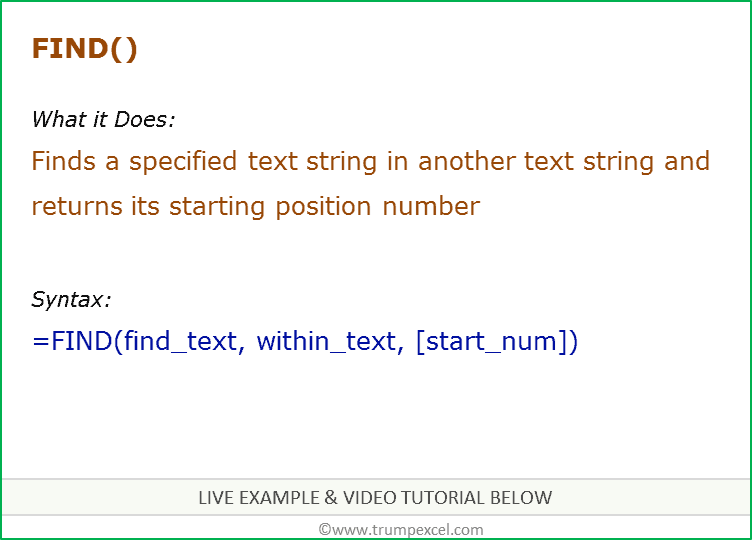
When to use Excel FIND Function
Excel FIND function can be used when you want to locate a text string within another text string and find its position.
What it Returns
It returns a number that represents the starting position of the string you are finding in another string.
Syntax
=FIND(find_text, within_text, [start_num])
Input Arguments
- find_text – the text or string that you need to find.
- within_text – the text within which you want to find the find_text argument.
- [start_num] – a number that represents the position from which you want the search to begin. If you omit it, it starts from the beginning.
Additional Notes
- If the start number is not specified, then it starts looking from the beginning of the string.
- Excel FIND function is case-sensitive. If you want to do a case-insensitive search, use Excel SEARCH function.
- Excel FIND function cannot handle wildcard characters. If you want to use wildcard characters, use the Excel SEARCH function.
- It returns a #VALUE! error if the searched string is not found in the text.
Excel FIND Function – Examples
Here are four examples of using Excel FIND function:
Searching for a Word in a Text String (from the beginning)
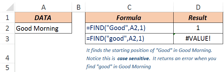
In the above example, when you look for the word Good in the text Good Morning, it returns 1, which is the position of the starting point of the searched word.
Note that Excel FIND function is case-sensitive. When you use good instead of Good, it returns a #VALUE! error.
If you are looking for a case-insensitive search, use Excel SEARCH function.
Finding a Word in a Text String (with a specified beginning)
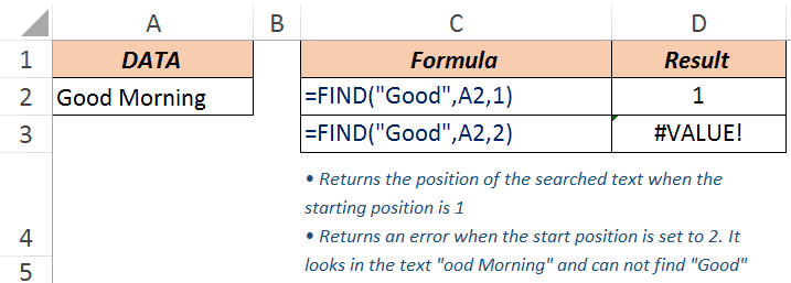
The third argument in the FIND function is the position within the text from where you want to start the search. In the example above, the function returns 1 when you search for the text Good in Good Morning and the starting position is 1.
However, it returns an error when you make it start at 2. Hence, it looks for the text Good in ood Morning. Since it can not find it, it returns an error.
Note: If you skip the last argument and don’t provide the starting position, by default it takes it as 1.
When there are Multiple Occurrence of the Searched Text
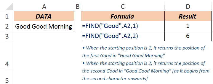
Excel FIND function starts looking in the specified text from the specified position. In the above example, when you look for the text Good in Good Good Morning with the starting position as 1, it returns 1, as it finds it at the beginning.
When you start the search from the second character onwards, it returns 6, as it finds the matching text at the sixth position.
Extracting Everything to the Left a Specified Character/String
Suppose you have the email ids do some superheroes as shown below and you want to extract only the username part (which would be the characters before the @).
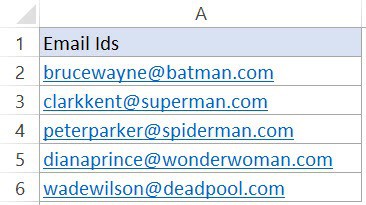
Below is the formula that will find the position of ‘@’ in each email id and extract all the characters to the left of it:
=LEFT(A2,FIND(“@”,A2,1)-1)

The FIND function in this formula gives the position of the ‘@’ character. The LEFT function that uses this position to extract the username.
For example, in the case of brucewayne@batman.com, the FIND function returns 11. LEFT function then uses FIND(“@”,A2,1)-1 as the second argument to get the username.
Note that 1 is subtracted from the value returned by the FIND function as we want to exclude the @ from the result of the LEFT function.
Excel FIND Function – VIDEO
Related Excel Functions:
- Excel LOWER Function.
- Excel UPPER Function.
- Excel PROPER Function.
- Excel REPLACE Function.
- Excel SEARCH Function.
- Excel SUBSTITUTE Function.
You May Also Like the Following Tutorials:
- How to Quickly Find and Remove Hyperlinks in Excel.
- How to Find Merged Cells in Excel.
- How to Find and Remove Duplicates in Excel.
- Using Find and Replace in Excel.
When working with Excel, we see so many peculiar situations. One of those situations is searching for the particular text in the cell. The first thing that comes to mind when we say we want to search for a specific text in the worksheet is the “Find and Replace” method in Excel, which is the most popular one. But Ctrl + F can find the text you are looking for but cannot go beyond that. So, for example, if the cell contains certain words, you may want the result in the next cell as “TRUE” or “FALSE.” So, Ctrl + F stops there.
Table of contents
- How to Search For Text in Excel?
- Which Formula Can Tell Us A Cell Contains Specific Text?
- Alternatives to FIND Function
- Alternative #1 – Excel Search Function
- Alternative #2 – Excel Countif Function
- Highlight the Cell which has Particular Text Value
- Recommended Articles
Here, we will take you through the formulas to search for the particular text in the cell value and arrive at the result.
You can download this Search For Text Excel Template here – Search For Text Excel Template
Which Formula Can Tell Us A Cell Contains Specific Text?
It is a question we have seen many times in Excel forums. The first formula that came to mind was the “FIND” function.
The FIND function can return the position of the supplied text values in the string. So, if the FIND method returns any number, then we can consider the cell as it has the text or else not.
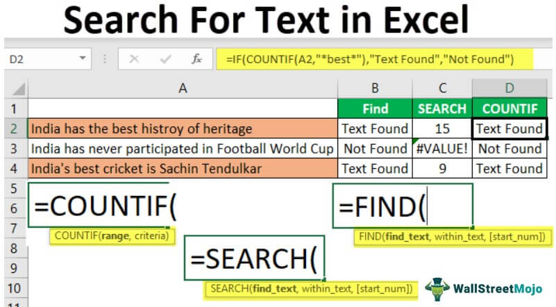
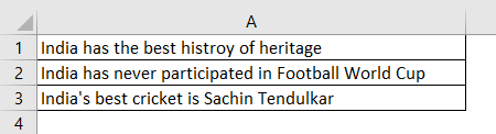
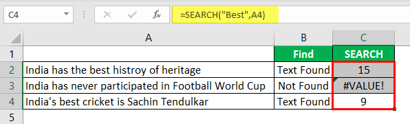
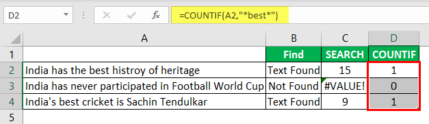
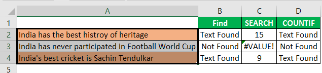
- For example, look at the below data.

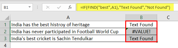
- In the above data, we have three sentences in three different rows. Now in each cell, we need to search for the text “Best.” So, apply the FIND function.

- The “find_text” argument mentions the text we need to find.

- For the “within_text,” select the full sentence, i.e., cell reference.

- The last parameter is not required to close the bracket and press the “Enter” key.

So, in two sentences, we have the word “best.” We can see the error value of #VALUE! in cell B2, which shows that cell A2 does not have the text value “best.”
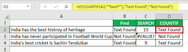
- Instead of numbers, we can also enter the result in our own words. For this, we need to use the IF condition.


So, in the IF condition, we have supplied the result as “Text Found” if the value “best” is found. Otherwise, we have provided the result as “Not Found.”
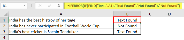
But, here we have a problem, even though we have supplied the result as “Not Found,” if the text is still not found, we are getting the error value as #VALUE!.
So, nobody wants to have an error value in their Excel sheet. Therefore, we must enclose the formula with the ISNUMERIC function to overcome this error value.

The ISNUMERIC function evaluates whether the FIND function returns the number or not. If the FIND function returns the number, it will supply TRUE to the IF condition or else FALSE condition. Based on the result provided by the ISNUMERIC function, the IF condition will return the result accordingly.
We can also use the IFERROR function in excelThe IFERROR function in Excel checks a formula (or a cell) for errors and returns a specified value in place of the error.read more to deal with error values instead of ISNUMERIC. For example, the below formula will also return “Not Found” if the FIND function returns the error value.
Alternatives to FIND Function
Alternative #1 – Excel Search Function
Instead of the FIND function, we can also use the SEARCH function in excelSearch function gives the position of a substring in a given string when we give a parameter of the position to search from. As a result, this formula requires three arguments. The first is the substring, the second is the string itself, and the last is the position to start the search.read more to search the particular text in the string. The syntax of the SEARCH function is the same as the FIND function.
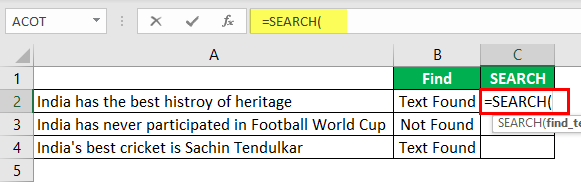
Supply the “find_text” as “Best.”
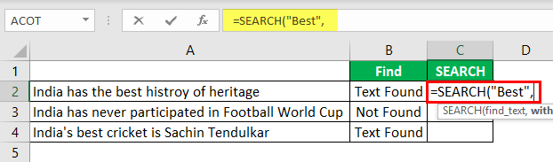
The “within_text” is our cell reference.
Even the SEARCH function returns an error value as #VALUE! If the finding text “best” is not found. As we have seen above, we need to enclose the formula with ISNUMERIC or IFERROR functions.
Alternative #2 – Excel Countif Function
Another way to search for a particular text is using the COUNTIF functionThe COUNTIF function in Excel counts the number of cells within a range based on pre-defined criteria. It is used to count cells that include dates, numbers, or text. For example, COUNTIF(A1:A10,”Trump”) will count the number of cells within the range A1:A10 that contain the text “Trump”
read more. This function works without any error.
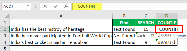
In the range, the argument selects the cell reference.
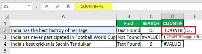
In the criteria column, we need to use a wildcard in excelIn Excel, wildcards are the three special characters asterisk, question mark, and tilde. Asterisk denotes multiple characters, a question mark denotes a single character, and a tilde denotes the identification of a wild card character.read more because we are just finding the part of the string value, so enclose the word “best” with an asterisk (*) wildcard.
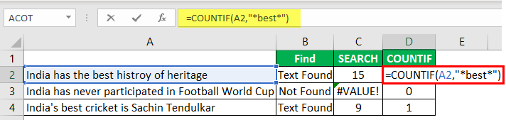
This formula will return the word “best” count in the selected cell value. Since we have only one “best” value, we will get only 1 as the count.
We can apply only the IF condition to get the result without error.
Highlight the Cell which has a Particular Text Value
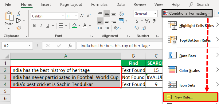
If you are not a fan of formulas, you can highlight the cell with a particular word. For example, to highlight the cell with the word “best,” we need to use conditional formatting in excelConditional formatting is a technique in Excel that allows us to format cells in a worksheet based on certain conditions. It can be found in the styles section of the Home tab.read more.
First, select the data cells and click “Conditional Formatting” > “New Rule.”
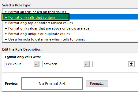
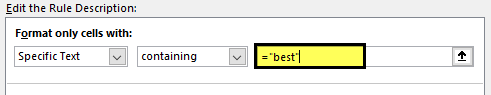
Under “New Rule,” select the “Format only cells that contain” option.
From the first dropdown, select “Specific Text.”

The formula section enters the text we search for in double quotes with the equal sign. =’best.’
Then, click on “FORMAT” and choose the formatting style.
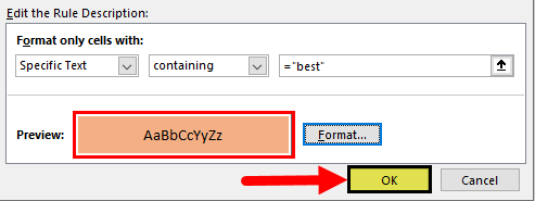
Click on “OK.” It will highlight all the cells which have the word “best.”
Using various techniques, we can search the particular text in Excel.
Recommended Articles
This article is a guide to Search For Text in Excel. Here, we discuss the top three methods to search the cell value for a specific text and arrive at the result with practical examples and a downloadable Excel template. You may learn more about Excel from the following articles: –
- Find Links in Excel
- Using Find and Select in Excel
- Search Box in Excel
Question: What formula tells you if A1 contains the text «apple»?
This is a surprisingly tricky problem in Excel. The «obvious» answer is to use the FIND function to «look» for the text, like this:
=FIND("apple",A1)
Then, if you want a TRUE/FALSE result, add the IF function:
=IF(FIND("apple",A1),TRUE)
This works great if «apple» is found – FIND returns a number to indicate the position, and IF calls it good and returns TRUE.
But FIND has an annoying quirk – if it doesn’t find «apple», it returns the #VALUE error. This means that the formula above doesn’t return FALSE when text isn’t found, it returns #VALUE:

FIND returns the position of the text (if found), but #VALUE if not found.

Unfortunately, this error appears even if we wrap the FIND function in the IF function.
Grrrr. Nobody likes to see errors in their spreadsheets.
(There may be some good reason for this, but returning zero would be much nicer.)
What about the SEARCH function, which also locates the position of text? Unlike FIND, SEARCH supports wildcards, and is not case-sensitive. Maybe SEARCH returns FALSE or zero if the text isn’t found?
Nope. SEARCH also returns #VALUE when the text isn’t found.
So, what to do? Well, in a classic, counter-intuitive Excel move, you can trap the #VALUE error with the ISNUMBER function, like this:
=ISNUMBER(FIND("apple",A1))
Now ISNUMBER returns TRUE when FIND yields a number, and FALSE when FIND throws the error.

Another way with COUNTIF
If all that seems a little crazy, you can also the COUNTIF function to find text:
=COUNTIF(A1,"*apple*")
It might seem strange to use COUNTIF like this, since we’re just counting one cell. But COUNTIF does the job well – if «apple» is found, it returns 1, if not, it returns zero.

For many situations (e.g. conditional formatting) a 1 or 0 result will be just fine. But if you want to force a TRUE/FALSE result, just wrap with IF:
=IF(COUNTIF(A1,"*apple*"),TRUE)
Now we get TRUE if «apple» is found, FALSE if not:

Note that COUNTIF supports wildcards – in fact, you must use wildcards to get the «contains» behavior, by adding an asterisk to either side of the text you’re looking for. On the downside, COUNTIF isn’t case-sensitive, so you’ll need to use FIND if case is important.
Other examples
So what can you do with these kind of formulas? A lot!
Here are a few examples (with full explanations) to inspire you:
- Count cells that contain specific text
- Sum cells that contain specific text
- Test a cell to see if contains one of many things
- Highlight cells that contain specific text
- Build a search box to highlight data (video)
Logical confusion?
If you need to brush up on how logical formulas work, see this video. It’s kind of boring, but it runs through a lot of examples.
Other formulas
If you like formulas (who doesn’t?!), we maintain a big list of examples.
Содержание
- Cell contains specific text
- Related functions
- Summary
- Generic formula
- Explanation
- SEARCH function (not case-sensitive)
- Wildcards
- FIND function (case-sensitive)
- If cell contains
- With hardcoded search string
- How to Extract the First Word from a Text String in Excel (3 Easy Ways)
- Extract the First Word Using Text Formulas
- Extract the First Word Using Find and Replace
- Extract the First Word Using Flash Fill
- Use Excel built-in functions to find data in a table or a range of cells
- Summary
- Create the Sample Worksheet
- Term Definitions
- Functions
- LOOKUP()
- VLOOKUP()
- INDEX() and MATCH()
- OFFSET() and MATCH()
Cell contains specific text
Summary
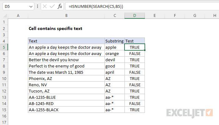
To check if a cell contains specific text (i.e. a substring), you can use the SEARCH function together with the ISNUMBER function. In the example shown, the formula in D5 is:
This formula returns TRUE if the substring is found, and FALSE if not. Note the SEARCH function is not case-sensitive. See below for a case-sensitive formula.
Generic formula
Explanation
In this example, the goal is to test a value in a cell to see if it contains a specific substring. Excel contains two functions designed to check the occurrence of one text string inside another: the SEARCH function and the FIND function. Both functions return the position of the substring if found as a number, and a #VALUE! error if the substring is not found. The difference is that the SEARCH function supports wildcards but is not case-sensitive, while the FIND function is case-sensitive but does not support wildcards. The general approach with either function is to use the ISNUMBER function to check for a numeric result (a match) and return TRUE or FALSE.
SEARCH function (not case-sensitive)
The SEARCH function is designed to look inside a text string for a specific substring. If SEARCH finds the substring, it returns a position of the substring in the text as a number. If the substring is not found, SEARCH returns a #VALUE error. For example:
To force a TRUE or FALSE result, we use the ISNUMBER function. ISNUMBER returns TRUE for numeric values and FALSE for anything else. So, if SEARCH finds the substring, it returns the position as a number, and ISNUMBER returns TRUE:
If SEARCH doesn’t find the substring, it returns an error, which causes the ISNUMBER to return FALSE.
Wildcards
Although SEARCH is not case-sensitive, it does support wildcards (*?
). For example, the question mark (?) wildcard matches any one character. The formula below looks for a 3-character substring beginning with «x» and ending in «y»:
The asterisk (*) wildcard matches zero or more characters. This wildcard is not as useful in the SEARCH function because SEARCH already looks for a substring. For example, it might seem like the following formula will test for a value that ends with «z»:
However, because SEARCH automatically looks for a substring, the following formulas all return 1 as a result, even though the text in the first formula is the only text that ends with «z»:
This means the asterisk (*) is not a reliable way to test for «ends with». However, you an use the the asterisk (*) wildcard like this:
Here we are looking for «x», «2», and «b» in that order, with any number of characters in between. Finally, you can use the tilde (
) as an escape character to indicate that the next character is a literal like this:
The above formulas use SEARCH to find a literal asterisk (*), question mark (?) , and tilde (
FIND function (case-sensitive)
Like the SEARCH function, the FIND function returns the position of a substring in text as a number, and an error if the substring is not found. However, unlike the SEARCH function, the FIND function respects case:
To make a case-sensitive version of the formula, just replace the SEARCH function with the FIND function in the formula above:
The result is a case-sensitive search:
If cell contains
To return a custom result when a cell contains specific text, add the IF function like this:
Instead of returning TRUE or FALSE, the formula above will return «Yes» if substring is found and «No» if not.
With hardcoded search string
To test for a hardcoded substring, enclose the text in double quotes («»). For example, to check A1 for the text «apple» use:
Источник
Excel has some wonderful formulas that can help you slice and dice the text data.
Sometimes, when you have the text data, you may want to extract the first word from the text string in a cell.
There are multiple ways you can do this in Excel (using a combination of formulas, using Find and Replace, and using Flash Fill)
In this tutorial, I will show you some really simple ways to extract the first word from a text string in Excel.
This Tutorial Covers:
Suppose you have the following dataset, where you want to get the first word from each cell.

The below formula will do this:

Let me explain how this formula works.
The FIND part of the formula is used to find the position of the space character in the text string. When the formula finds the position of the space character, the LEFT function is used to extract all the characters before that first space character in the text string.
While the LEFT formula alone should be enough, it will give you an error in case there is only one word in the cell and no space characters.
To handle this situation, I have wrapped the LEFT formula in the IFERROR formula, which simply returns the original cell content (as there are no space characters indicating that it’s either empty or has only one word).
One good thing about this method is that the result is dynamic. This means that in case you change the original text string in the cells in column A, the formula in column B will automatically update and give the correct result.
In case you don’t want the formula, you can convert it into values.
Extract the First Word Using Find and Replace
Another quick method to extract the first word is to use Find and Replace to remove everything except the first word.
Suppose you have the dataset as shown below:
Below are the steps to use Find and Replace to only get the first word and remove everything else:
- Copy the text from column A to column B. This is to make sure that we have the original data as well.
- Select all the cells in Column B where you want to get the first word
- Click the Home tab
- In the Editing group, click on Find and Select option and then click on Replace. This will open the Find & Replace dialog box.
- In the Find what field, enter * (one space character followed by the asterisk sign)
- Leave the Replace with field empty
- Click on Replace All button.


The above steps would remove everything except the first word in the cells.

How does this work?
In Find what field, we have used a space character followed by the asterisk sign. The asterisk sign (*) is a wild card character that represents any number of characters.
So when we ask Excel to find cells that contain space character followed by the asterisk sign and replace it with blank, it finds the first space character and removes everything after it – leaving us with the first word only.
And in case you a cell that has no text or only one word with no space characters, the above steps would not make any changes to it.
Another really simple and fast method to extract the first word using Flash Fill.
Flash Fill was introduced in Excel 2013 and is available in all the versions after that. It helps in text manipulation by identifying the pattern that you’re trying to achieve and fills it for the entire column.
For example, suppose you have the below dataset and you want to only extract the first word.
Below are the steps to do this:
- In cell B2, which is the adjacent column of our data, manually enter ‘Marketing’ (which is the expected result)
- In cell B3, enter ‘HR’
- Select the range B2:B10
- Click on the Home tab
- In the Editing group, click on the Fill drop-down
- Click on Flash Fill option


The above steps would fill all the cells with the first word from the adjacent column (column A).
Note: When typing the expected result in the second cell in column B, you may see all text in all the cells in a light gray color. That is the result you will get if you hit the enter key right away. In case you don’t see the gray line, use the Flash Fill option in the ribbon.
So these are three simple methods to extract the first word from a text string in Excel.
I hope you found this tutorial useful!
Other Excel tutorials you may like:
Источник
Use Excel built-in functions to find data in a table or a range of cells
Summary
This step-by-step article describes how to find data in a table (or range of cells) by using various built-in functions in Microsoft Excel. You can use different formulas to get the same result.
Create the Sample Worksheet
This article uses a sample worksheet to illustrate Excel built-in functions. Consider the example of referencing a name from column A and returning the age of that person from column C. To create this worksheet, enter the following data into a blank Excel worksheet.
You will type the value that you want to find into cell E2. You can type the formula in any blank cell in the same worksheet.
Term Definitions
This article uses the following terms to describe the Excel built-in functions:
The whole lookup table
The value to be found in the first column of Table_Array.
Lookup_Array
-or-
Lookup_Vector
The range of cells that contains possible lookup values.
The column number in Table_Array the matching value should be returned for.
3 (third column in Table_Array)
Result_Array
-or-
Result_Vector
A range that contains only one row or column. It must be the same size as Lookup_Array or Lookup_Vector.
A logical value (TRUE or FALSE). If TRUE or omitted, an approximate match is returned. If FALSE, it will look for an exact match.
This is the reference from which you want to base the offset. Top_Cell must refer to a cell or range of adjacent cells. Otherwise, OFFSET returns the #VALUE! error value.
This is the number of columns, to the left or right, that you want the upper-left cell of the result to refer to. For example, «5» as the Offset_Col argument specifies that the upper-left cell in the reference is five columns to the right of reference. Offset_Col can be positive (which means to the right of the starting reference) or negative (which means to the left of the starting reference).
Functions
LOOKUP()
The LOOKUP function finds a value in a single row or column and matches it with a value in the same position in a different row or column.
The following is an example of LOOKUP formula syntax:
The following formula finds Mary’s age in the sample worksheet:
The formula uses the value «Mary» in cell E2 and finds «Mary» in the lookup vector (column A). The formula then matches the value in the same row in the result vector (column C). Because «Mary» is in row 4, LOOKUP returns the value from row 4 in column C (22).
NOTE: The LOOKUP function requires that the table be sorted.
For more information about the LOOKUP function, click the following article number to view the article in the Microsoft Knowledge Base:
VLOOKUP()
The VLOOKUP or Vertical Lookup function is used when data is listed in columns. This function searches for a value in the left-most column and matches it with data in a specified column in the same row. You can use VLOOKUP to find data in a sorted or unsorted table. The following example uses a table with unsorted data.
The following is an example of VLOOKUP formula syntax:
The following formula finds Mary’s age in the sample worksheet:
The formula uses the value «Mary» in cell E2 and finds «Mary» in the left-most column (column A). The formula then matches the value in the same row in Column_Index. This example uses «3» as the Column_Index (column C). Because «Mary» is in row 4, VLOOKUP returns the value from row 4 in column C (22).
For more information about the VLOOKUP function, click the following article number to view the article in the Microsoft Knowledge Base:
INDEX() and MATCH()
You can use the INDEX and MATCH functions together to get the same results as using LOOKUP or VLOOKUP.
The following is an example of the syntax that combines INDEX and MATCH to produce the same results as LOOKUP and VLOOKUP in the previous examples:
The following formula finds Mary’s age in the sample worksheet:
The formula uses the value «Mary» in cell E2 and finds «Mary» in column A. It then matches the value in the same row in column C. Because «Mary» is in row 4, the formula returns the value from row 4 in column C (22).
NOTE: If none of the cells in Lookup_Array match Lookup_Value («Mary»), this formula will return #N/A.
For more information about the INDEX function, click the following article number to view the article in the Microsoft Knowledge Base:
OFFSET() and MATCH()
You can use the OFFSET and MATCH functions together to produce the same results as the functions in the previous example.
The following is an example of syntax that combines OFFSET and MATCH to produce the same results as LOOKUP and VLOOKUP:
This formula finds Mary’s age in the sample worksheet:
The formula uses the value «Mary» in cell E2 and finds «Mary» in column A. The formula then matches the value in the same row but two columns to the right (column C). Because «Mary» is in column A, the formula returns the value in row 4 in column C (22).
For more information about the OFFSET function, click the following article number to view the article in the Microsoft Knowledge Base:
Источник