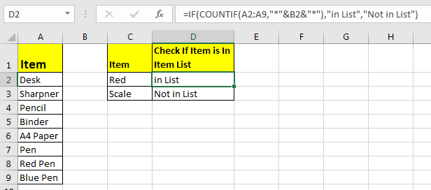
So, there are times when you would like to know that a value is in a list or not. We have done this using VLOOKUP. But we can do the same thing using COUNTIF function too. So in this article, we will learn how to check if a values is in a list or not using various ways.
Check If Value In Range Using COUNTIF Function
So as we know, using COUNTIF function in excel we can know how many times a specific value occurs in a range. So if we count for a specific value in a range and its greater than zero, it would mean that it is in the range. Isn’t it?
Generic Formula
=COUNTIF(range,value)>0
Range: The range in which you want to check if the value exist in range or not.
Value: The value that you want to check in the range.
Let’s see an example:
Excel Find Value is in Range Example
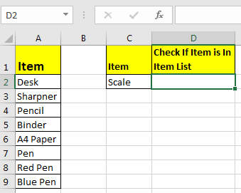
For this example, we have below sample data. We need a check-in the cell D2, if the given item in C2 exists in range A2:A9 or say item list. If it’s there then, print TRUE else FALSE.
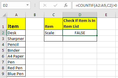
Write this formula in cell D2:
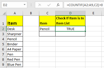
Since C2 contains “scale” and it’s not in the item list, it shows FALSE. Exactly as we wanted. Now if you replace “scale” with “Pencil” in the formula above, it’ll show TRUE.
Now, this TRUE and FALSE looks very back and white. How about customizing the output. I mean, how about we show, “found” or “not found” when value is in list and when it is not respectively.
Since this test gives us TRUE and FALSE, we can use it with IF function of excel.
Write this formula:
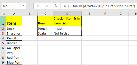
=IF(COUNTIF(A2:A9,C2)>0,»in List»,»Not in List»)
You will have this as your output.
What If you remove “>0” from this if formula?
=IF(COUNTIF(A2:A9,C2),»in List»,»Not in List»)
It will work fine. You will have same result as above. Why? Because IF function in excel treats any value greater than 0 as TRUE.
How to check if a value is in Range with Wild Card Operators
Sometimes you would want to know if there is any match of your item in the list or not. I mean when you don’t want an exact match but any match.
For example, if in the above-given list, you want to check if there is anything with “red”. To do so, write this formula.
=IF(COUNTIF(A2:A9,»*red*»),»in List»,»Not in List»)
This will return a TRUE since we have “red pen” in our list. If you replace red with pink it will return FALSE. Try it.
Now here I have hardcoded the value in list but if your value is in a cell, say in our favourite cell B2 then write this formula.
IF(COUNTIF(A2:A9,»*»&B2&»*»),»in List»,»Not in List»)
There’s one more way to do the same. We can use the MATCH function in excel to check if the column contains a value. Let’s see how.
Find if a Value is in a List Using MATCH Function
So as we all know that MATCH function in excel returns the index of a value if found, else returns #N/A error. So we can use the ISNUMBER to check if the function returns a number.
If it returns a number ISNUMBER will show TRUE, which means it’s found else FALSE, and you know what that means.
Write this formula in cell C2:
=ISNUMBER(MATCH(C2,A2:A9,0))
The MATCH function looks for an exact match of value in cell C2 in range A2:A9. Since DESK is on the list, it shows a TRUE value and FALSE for SCALE.
So yeah, these are the ways, using which you can find if a value is in the list or not and then take action on them as you like using IF function. I explained how to find value in a range in the best way possible. Let me know if you have any thoughts. The comments section is all yours.
Related Articles:
How to Check If Cell Contains Specific Text in Excel
How to Check A list of Texts In String in Excel
How to take the Average Difference between lists in Excel
How to Get Every Nth Value From A list in Excel
Popular Articles:
50 Excel Shortcuts to Increase Your Productivity
How to use the VLOOKUP Function in Excel
How to use the COUNTIF function in Excel
How to use the SUMIF Function in Excel
Summary
This step-by-step article describes how to find data in a table (or range of cells) by using various built-in functions in Microsoft Excel. You can use different formulas to get the same result.
Create the Sample Worksheet
This article uses a sample worksheet to illustrate Excel built-in functions. Consider the example of referencing a name from column A and returning the age of that person from column C. To create this worksheet, enter the following data into a blank Excel worksheet.
You will type the value that you want to find into cell E2. You can type the formula in any blank cell in the same worksheet.
|
A |
B |
C |
D |
E |
||
|
1 |
Name |
Dept |
Age |
Find Value |
||
|
2 |
Henry |
501 |
28 |
Mary |
||
|
3 |
Stan |
201 |
19 |
|||
|
4 |
Mary |
101 |
22 |
|||
|
5 |
Larry |
301 |
29 |
Term Definitions
This article uses the following terms to describe the Excel built-in functions:
|
Term |
Definition |
Example |
|
Table Array |
The whole lookup table |
A2:C5 |
|
Lookup_Value |
The value to be found in the first column of Table_Array. |
E2 |
|
Lookup_Array |
The range of cells that contains possible lookup values. |
A2:A5 |
|
Col_Index_Num |
The column number in Table_Array the matching value should be returned for. |
3 (third column in Table_Array) |
|
Result_Array |
A range that contains only one row or column. It must be the same size as Lookup_Array or Lookup_Vector. |
C2:C5 |
|
Range_Lookup |
A logical value (TRUE or FALSE). If TRUE or omitted, an approximate match is returned. If FALSE, it will look for an exact match. |
FALSE |
|
Top_cell |
This is the reference from which you want to base the offset. Top_Cell must refer to a cell or range of adjacent cells. Otherwise, OFFSET returns the #VALUE! error value. |
|
|
Offset_Col |
This is the number of columns, to the left or right, that you want the upper-left cell of the result to refer to. For example, «5» as the Offset_Col argument specifies that the upper-left cell in the reference is five columns to the right of reference. Offset_Col can be positive (which means to the right of the starting reference) or negative (which means to the left of the starting reference). |
Functions
LOOKUP()
The LOOKUP function finds a value in a single row or column and matches it with a value in the same position in a different row or column.
The following is an example of LOOKUP formula syntax:
=LOOKUP(Lookup_Value,Lookup_Vector,Result_Vector)
The following formula finds Mary’s age in the sample worksheet:
=LOOKUP(E2,A2:A5,C2:C5)
The formula uses the value «Mary» in cell E2 and finds «Mary» in the lookup vector (column A). The formula then matches the value in the same row in the result vector (column C). Because «Mary» is in row 4, LOOKUP returns the value from row 4 in column C (22).
NOTE: The LOOKUP function requires that the table be sorted.
For more information about the LOOKUP function, click the following article number to view the article in the Microsoft Knowledge Base:
How to use the LOOKUP function in Excel
VLOOKUP()
The VLOOKUP or Vertical Lookup function is used when data is listed in columns. This function searches for a value in the left-most column and matches it with data in a specified column in the same row. You can use VLOOKUP to find data in a sorted or unsorted table. The following example uses a table with unsorted data.
The following is an example of VLOOKUP formula syntax:
=VLOOKUP(Lookup_Value,Table_Array,Col_Index_Num,Range_Lookup)
The following formula finds Mary’s age in the sample worksheet:
=VLOOKUP(E2,A2:C5,3,FALSE)
The formula uses the value «Mary» in cell E2 and finds «Mary» in the left-most column (column A). The formula then matches the value in the same row in Column_Index. This example uses «3» as the Column_Index (column C). Because «Mary» is in row 4, VLOOKUP returns the value from row 4 in column C (22).
For more information about the VLOOKUP function, click the following article number to view the article in the Microsoft Knowledge Base:
How to Use VLOOKUP or HLOOKUP to find an exact match
INDEX() and MATCH()
You can use the INDEX and MATCH functions together to get the same results as using LOOKUP or VLOOKUP.
The following is an example of the syntax that combines INDEX and MATCH to produce the same results as LOOKUP and VLOOKUP in the previous examples:
=INDEX(Table_Array,MATCH(Lookup_Value,Lookup_Array,0),Col_Index_Num)
The following formula finds Mary’s age in the sample worksheet:
=INDEX(A2:C5,MATCH(E2,A2:A5,0),3)
The formula uses the value «Mary» in cell E2 and finds «Mary» in column A. It then matches the value in the same row in column C. Because «Mary» is in row 4, the formula returns the value from row 4 in column C (22).
NOTE: If none of the cells in Lookup_Array match Lookup_Value («Mary»), this formula will return #N/A.
For more information about the INDEX function, click the following article number to view the article in the Microsoft Knowledge Base:
How to use the INDEX function to find data in a table
OFFSET() and MATCH()
You can use the OFFSET and MATCH functions together to produce the same results as the functions in the previous example.
The following is an example of syntax that combines OFFSET and MATCH to produce the same results as LOOKUP and VLOOKUP:
=OFFSET(top_cell,MATCH(Lookup_Value,Lookup_Array,0),Offset_Col)
This formula finds Mary’s age in the sample worksheet:
=OFFSET(A1,MATCH(E2,A2:A5,0),2)
The formula uses the value «Mary» in cell E2 and finds «Mary» in column A. The formula then matches the value in the same row but two columns to the right (column C). Because «Mary» is in column A, the formula returns the value in row 4 in column C (22).
For more information about the OFFSET function, click the following article number to view the article in the Microsoft Knowledge Base:
How to use the OFFSET function
Need more help?
I have two columns in Excel, and I want to find (preferably highlight) the items that are in column B but not in column A.
What’s the quickest way to do this?
Excellll
12.5k11 gold badges50 silver badges78 bronze badges
asked Dec 10, 2009 at 18:44
- Select the list in column A
- Right-Click and select Name a Range…
- Enter «ColumnToSearch»
- Click cell C1
- Enter this formula:
=MATCH(B1,ColumnToSearch,0) - Drag the formula down for all items in B
If the formula fails to find a match, it will be marked #N/A, otherwise it will be a number.
If you’d like it to be TRUE for match and FALSE for no match, use this formula instead:
=ISNUMBER(MATCH(B1,ColumnToSearch,0))
If you’d like to return the unfound value and return empty string for found values
=IF(ISNUMBER(MATCH(B1,ColumnToSearch,0)),"",B1)
answered Dec 10, 2009 at 19:01
devuxerdevuxer
3,9316 gold badges31 silver badges33 bronze badges
6
Here’s a quick-and-dirty method.
Highlight Column B and open Conditional Formatting.
Pick Use a formula to determine which cells to highlight.
Enter the following formula then set your preferred format.
=countif(A:A,B1)=0
Excellll
12.5k11 gold badges50 silver badges78 bronze badges
answered May 9, 2011 at 16:18
EllesaEllesa
10.8k2 gold badges38 silver badges52 bronze badges
2
Select the two columns. Go to Conditional Formatting and select Highlight Cell Rules. Select Duplicate values. When you get to the next step you can change it to unique values. I just did it and it worked for me.
answered Apr 16, 2015 at 20:02
DOB DOB
2813 silver badges2 bronze badges
4
Took me forever to figure this out but it’s very simple. Assuming data begins in A2 and B2 (for headers) enter this formula in C2:
=MATCH(B2,$A$2:$A$287,0)
Then click and drag down.
A cell with #N/A means that the value directly next to it in column B does not show up anywhere in the entire column A.
Please note that you need to change $A$287 to match your entire search array in Column A. For instance if your data in column A goes down for 1000 entries it should be $A$1000.
n.st
1,8781 gold badge17 silver badges30 bronze badges
answered Dec 6, 2013 at 20:43
brentonbrenton
1711 silver badge2 bronze badges
1
See my array formula answer to listing A not found in B here:
=IFERROR(INDEX($A$2:$A$1999,MATCH(0,IFERROR(MATCH($A$2:$A$1999,$B$2:$B$399,0),COUNTIF($C$1:$C1,$A$2:$A$1999)),0)),»»)
Comparing two columns of names and returning missing names
C. Ross
6,06416 gold badges60 silver badges82 bronze badges
answered Oct 21, 2011 at 14:02
1
My requirements was not to highlight but to show all values except that are duplicates amongst 2 columns. I took help of @brenton’s solution and further improved to show the values so that I can use the data directly:
=IF(ISNA(MATCH(B2,$A$2:$A$2642,0)), A2, "")
Copy this in the first cell of the 3rd column and apply the formula through out the column so that it will list all items from column B there are not listed in column A.
answered Feb 24, 2014 at 11:10
1
Thank you to those who have shared their answers. Because of your solutions, I was able to make my way to my own.
In my version of this question, I had two columns to compare — a full graduating class (Col A) and a subset of that graduating class (Col B). I wanted to be able to highlight in the full graduating class those students who were members of the subset.
I put the following formula into a third column:
=if(A2=LOOKUP(A2,$B$2:$B$91),1100,0)
This coded most of my students, though it yielded some errors in the first few rows of data.
answered Sep 11, 2014 at 13:25
in C1 write =if(A1=B1 , 0, 1). Then in Conditional formatting, select Data bars or Color scales. It’s the easiest way.
Jawa
3,60913 gold badges31 silver badges36 bronze badges
answered Feb 16, 2015 at 9:52
Explanation
The COUNTIF function counts cells that meet criteria, returning the number of occurrences found. If no cells meet criteria, COUNTIF returns zero. You can use behavior directly inside an IF statement to mark values that have a zero count (i.e. values that are missing). In the example shown, the formula in G6 is:
=IF(COUNTIF(list,F6),"OK","Missing")
where «list» is a named range that corresponds to the range B6:B11.
The IF function requires a logical test to return TRUE or FALSE. In this case, the COUNTIF function performs the logical test. If the value is found in list, COUNTIF returns a number directly to the IF function. This result could be any number… 1, 2, 3, etc.
The IF function will evaluate any number as TRUE, causing IF to return «OK». If the value is not found in list, COUNTIF returns zero (0), which evaluates as FALSE, and IF returns «Missing».
Alternative with MATCH
You can also test for missing values using the MATCH function. MATCH finds the position of an item in a list and will return the #N/A error when a value is not found. You can use this behavior to build a formula that returns «Missing» or «OK» by testing the result of MATCH with the ISNA function. ISNA returns TRUE only when it receives the #N/A error.
To use MATCH as shown in the example above, the formula is:
=IF(ISNA(MATCH(F6,list,0)),"Missing","OK")
Note that MATCH must be configured for exact match. To do this, make sure the third argument is zero or FALSE.
Alternative with VLOOKUP
Since VLOOKUP also returns an #N/A error when a value isn’t round, you can build a formula with VLOOKUP that works the same as the MATCH option. As with MATCH, you must configure VLOOKUP to use exact match, then test the result with ISNA. Also note that we only give VLOOKUP a single column (column B) for the table array.
We often compare one range values with another range to check for duplicates. But how to check if one range values exist in another range in Excel? We will learn in this article how to check if a range contains a value not in another range in Excel.

Formula Syntax
The generic formula syntax is;
=SUMPRODUCT(--(ISNA(MATCH(range1,range2,0))))>0
In this formula, we use the SUMPRODUCT function along with MATCH and ISNA function. This formula checks if range one contains at least one or more values that are not part of another range and returns TRUE, else it returns FALSE.

Suppose we have two lists of students’ roll numbers and we want to check if List A contains any values (one or more values) that are not in List B. Hence, the formula compares List A (range B2: B11) with List B (range C2: C11) and returns TRUE if List A contains at least one or more values not in List B, such as;
=SUMPRODUCT(--(ISNA(MATCH(B2:B11,C2:C11,0))))>0

How Formula Works
The MATCH function returns the relative positions of range B2: B11 values that exactly match in range C2: C11, and returns the #NA error value(s) where range B2: B11 values are not found in range C2: C11 as an array. Select the MATCH part of the formula in the formula bar and press F9 to view the resulting array.

The ISNA function checks for the #NA error values and returns TRUE, else returns FALSE. Hence, it converts the array returned by the MATCH function into an array of TRUE and FALSE logical values, such as;

The double dash (–) symbol converts the TRUE and FALSE logical values into an array of 1s and 0s. The SUMPRODUCT function sums this final array of 1s and 0s and compares the result with 0 and returns TRUE if the sum of values is greater than 0.


Instant Connection to an Expert through our Excelchat Service:
Most of the time, the problem you will need to solve will be more complex than a simple application of a formula or function. If you want to save hours of research and frustration, try our live Excelchat service! Our Excel Experts are available 24/7 to answer any Excel question you may have. We guarantee a connection within 30 seconds and a customized solution within 20 minutes.

