
Summary
This step-by-step article describes how to find data in a table (or range of cells) by using various built-in functions in Microsoft Excel. You can use different formulas to get the same result.
Create the Sample Worksheet
This article uses a sample worksheet to illustrate Excel built-in functions. Consider the example of referencing a name from column A and returning the age of that person from column C. To create this worksheet, enter the following data into a blank Excel worksheet.
You will type the value that you want to find into cell E2. You can type the formula in any blank cell in the same worksheet.
|
A |
B |
C |
D |
E |
||
|
1 |
Name |
Dept |
Age |
Find Value |
||
|
2 |
Henry |
501 |
28 |
Mary |
||
|
3 |
Stan |
201 |
19 |
|||
|
4 |
Mary |
101 |
22 |
|||
|
5 |
Larry |
301 |
29 |
Term Definitions
This article uses the following terms to describe the Excel built-in functions:
|
Term |
Definition |
Example |
|
Table Array |
The whole lookup table |
A2:C5 |
|
Lookup_Value |
The value to be found in the first column of Table_Array. |
E2 |
|
Lookup_Array |
The range of cells that contains possible lookup values. |
A2:A5 |
|
Col_Index_Num |
The column number in Table_Array the matching value should be returned for. |
3 (third column in Table_Array) |
|
Result_Array |
A range that contains only one row or column. It must be the same size as Lookup_Array or Lookup_Vector. |
C2:C5 |
|
Range_Lookup |
A logical value (TRUE or FALSE). If TRUE or omitted, an approximate match is returned. If FALSE, it will look for an exact match. |
FALSE |
|
Top_cell |
This is the reference from which you want to base the offset. Top_Cell must refer to a cell or range of adjacent cells. Otherwise, OFFSET returns the #VALUE! error value. |
|
|
Offset_Col |
This is the number of columns, to the left or right, that you want the upper-left cell of the result to refer to. For example, «5» as the Offset_Col argument specifies that the upper-left cell in the reference is five columns to the right of reference. Offset_Col can be positive (which means to the right of the starting reference) or negative (which means to the left of the starting reference). |
Functions
LOOKUP()
The LOOKUP function finds a value in a single row or column and matches it with a value in the same position in a different row or column.
The following is an example of LOOKUP formula syntax:
=LOOKUP(Lookup_Value,Lookup_Vector,Result_Vector)
The following formula finds Mary’s age in the sample worksheet:
=LOOKUP(E2,A2:A5,C2:C5)
The formula uses the value «Mary» in cell E2 and finds «Mary» in the lookup vector (column A). The formula then matches the value in the same row in the result vector (column C). Because «Mary» is in row 4, LOOKUP returns the value from row 4 in column C (22).
NOTE: The LOOKUP function requires that the table be sorted.
For more information about the LOOKUP function, click the following article number to view the article in the Microsoft Knowledge Base:
How to use the LOOKUP function in Excel
VLOOKUP()
The VLOOKUP or Vertical Lookup function is used when data is listed in columns. This function searches for a value in the left-most column and matches it with data in a specified column in the same row. You can use VLOOKUP to find data in a sorted or unsorted table. The following example uses a table with unsorted data.
The following is an example of VLOOKUP formula syntax:
=VLOOKUP(Lookup_Value,Table_Array,Col_Index_Num,Range_Lookup)
The following formula finds Mary’s age in the sample worksheet:
=VLOOKUP(E2,A2:C5,3,FALSE)
The formula uses the value «Mary» in cell E2 and finds «Mary» in the left-most column (column A). The formula then matches the value in the same row in Column_Index. This example uses «3» as the Column_Index (column C). Because «Mary» is in row 4, VLOOKUP returns the value from row 4 in column C (22).
For more information about the VLOOKUP function, click the following article number to view the article in the Microsoft Knowledge Base:
How to Use VLOOKUP or HLOOKUP to find an exact match
INDEX() and MATCH()
You can use the INDEX and MATCH functions together to get the same results as using LOOKUP or VLOOKUP.
The following is an example of the syntax that combines INDEX and MATCH to produce the same results as LOOKUP and VLOOKUP in the previous examples:
=INDEX(Table_Array,MATCH(Lookup_Value,Lookup_Array,0),Col_Index_Num)
The following formula finds Mary’s age in the sample worksheet:
=INDEX(A2:C5,MATCH(E2,A2:A5,0),3)
The formula uses the value «Mary» in cell E2 and finds «Mary» in column A. It then matches the value in the same row in column C. Because «Mary» is in row 4, the formula returns the value from row 4 in column C (22).
NOTE: If none of the cells in Lookup_Array match Lookup_Value («Mary»), this formula will return #N/A.
For more information about the INDEX function, click the following article number to view the article in the Microsoft Knowledge Base:
How to use the INDEX function to find data in a table
OFFSET() and MATCH()
You can use the OFFSET and MATCH functions together to produce the same results as the functions in the previous example.
The following is an example of syntax that combines OFFSET and MATCH to produce the same results as LOOKUP and VLOOKUP:
=OFFSET(top_cell,MATCH(Lookup_Value,Lookup_Array,0),Offset_Col)
This formula finds Mary’s age in the sample worksheet:
=OFFSET(A1,MATCH(E2,A2:A5,0),2)
The formula uses the value «Mary» in cell E2 and finds «Mary» in column A. The formula then matches the value in the same row but two columns to the right (column C). Because «Mary» is in column A, the formula returns the value in row 4 in column C (22).
For more information about the OFFSET function, click the following article number to view the article in the Microsoft Knowledge Base:
How to use the OFFSET function
Need more help?
We have the table in which the sales volumes of certain products are recorded in different months. It is necessary to find the data in the table, and the search criteria will be the headings of rows and columns. But the search must be performed separately by the range of the row or column. That is, only one of the criteria will be used. Therefore, you can`t apply the INDEX function here, but you need a special formula.
Finding values in the Excel table
To solve this problem, let us illustrate the example in the schematic table that corresponds to the conditions are described above.
The sheet with the table to search for values vertically and horizontally:
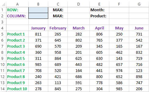
Above this table we can see the row with results. In the cell B1 we introduce the criterion for the search query, that is, the column header or the ROW name. And in the cell D1, to a search formula should return to the result of the calculation of the corresponding value. Then the second formula will work in the cell F1. She will already use the values of the cells B1 and D1 as the criteria for searching of the corresponding month.
Search of the value in the Excel ROW
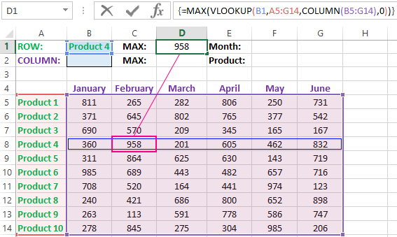
Now we are learning, in what maximum volume and in what month has been the maximum sale of the Product 4.
To search by columns:
- In the cell B1 you need to enter the value of the Product 4 — the name of the row, that will act as the criterion.
- In the cell D1 you need to enter the following:
- To confirm after entering the formula, you need to press the CTRL + SHIFT + Enter hotkey combination, because she must be executed in the array. If everything is done correctly, the curly braces will appear in the formula ROW.
- In the cell F1 you need to enter the second:
- For confirmation, to press the key combination CTRL + SHIFT + Enter again.
So we have found, in what month and what was the largest sale of the Product 4 for two quarters.
The principle of the formula for finding the value in the Excel ROW:
In the first argument of the VLOOKUP function (Vertical Look Up), indicates to the reference to the cell, where the search criterion is located. In the second argument indicates to the range of the cells for viewing during in the process of searching.
In the third argument of the VLOOKUP function should be indicated the number of the column from which you should to take the value against of the row named the Item 4. But since we do not previously know this number, we use the COLUMN function for creating the array of column numbers for the range B4:G15.
This allows the VLOOKUP function to collect the whole array of values. As a result, all relevant values are stored in memory for each column in the row Product 4 (namely: 360; 958; 201; 605; 462; 832). After that, the MAX function will only take the maximum number from this array and return it as the value for the cell D1, as the result of calculating.
As you can see, the construction of the formula is simple and concise. On its basis, it is possible in a similar way to find other indicators for a certain product. For example, the minimum or an average value of sales volume you need to find using for this purpose MIN or AVERAGE functions. Nothing hinders you from applying this skeleton of the formula to apply with more complex functions for implementation the most comfortable analysis of the sales report.
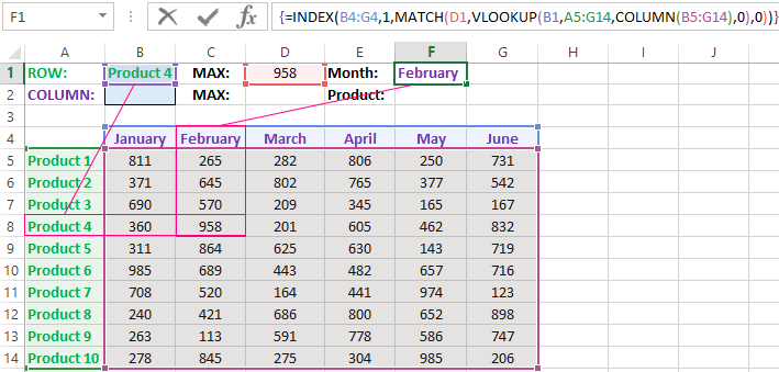
How can I get to the column headings from a single cell value?
For example, how effectively we displayed the month with the maximum sale, using of the second. It’s not difficult to notice that in the second formula we used the skeleton of the first formula without the MAX function. The main structure of the function is: VLOOKUP. We replaced the MAX on the MATCH, which in the first argument uses the value obtained by the previous formula. It acts as the criterion for searching for the month now.
And as a result, the MATCH function returns the column number 2, where the maximum value of the sales volume for the product is located for the product 4. After that, the INDEX function is included in the work. This function returns the value by the number of terms and column from the range specified in its arguments. Because the we have the number of column 2, and the row number in the range where the names of months are stored in any cases will be the value 1. Then we have the INDEX function to get the corresponding value from the range of B4:G4 — February (the second month).
Search the value in the Excel column
The second version of the task will be searching in the table with using the month name as the criterion. In such cases, we have to change the skeleton of our formula: the VLOOKUP function is replaced by the HLOOKUP (Horizontal Look Up) one, and the COLUMN function is replaced by the row one.
This will allow us to know what volume and what of the product the maximum sale was in a certain month.
To find what kind of the product had the maximum sales in a certain month, you should:
- In the cell B2 to enter the name of the month June — this value will be used as the search criterion.
- In the cell D2, you should to enter the formula:
- To confirm after entering the formula you need to press the combination of keys CTRL + SHIFT + Enter, as this formula will be executed in the array. And the curly braces will appear in the function ROW.
- In the cell F1, you need to enter the second:
- You need to click CTRL + SHIFT + Enter for confirmation again.
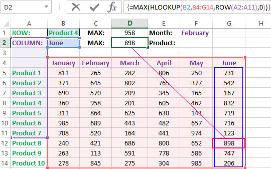
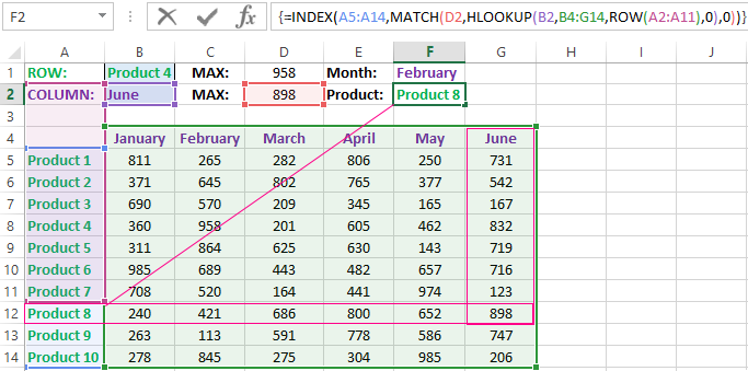
The principle of the formula for finding the value in the Excel column
In the first argument of the HLOOKUP function, we indicate to the reference by the cell with the criterion for the search. In the second argument specifies the reference to the table argument being scanned. The third argument is generated by the ROW function, what creates in the array of ROW numbers of 10 elements in memory. So there are 10 rows in the table section.
Further the HLOOKUP function, alternately using to each number of the row, creates the array of corresponding sales values from the table for the certain month (June). Further, the MAX function is left only to select the maximum value from this array.
Then just a little modifying to the first formula by using the INDEX and MATCH functions, we created the second function to display the names of the table rows according to the cell value. The names of the corresponding rows (products) we output in F2.
ATTENTION! When using the formula skeleton for other tasks, you need always to pay attention to the second and the third argument of the search HLOOKUP function. The number of covered rows in the range is specified in the argument, must match with the number of rows in the table. And also the numbering should begin with the second ROW!
Download example search values in the columns and rows
Read also: The searching of the value in a range Excel table in columns and rows
Indeed, the content of the range generally we don’t care — we just need the row counter. That is, you need to change the arguments to: ROW(B2:B11) or ROW(C2:C11) — this does not affect in the quality of the formula. The main thing is that — there are 10 rows in these ranges, as well as in the table. And the numbering starts from the second row!
Return to Excel Formulas List
Download Example Workbook
Download the example workbook
This tutorial will demonstrate how to find a number in a column or workbook in Excel and Google Sheets.
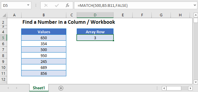
Find a Number in a Column
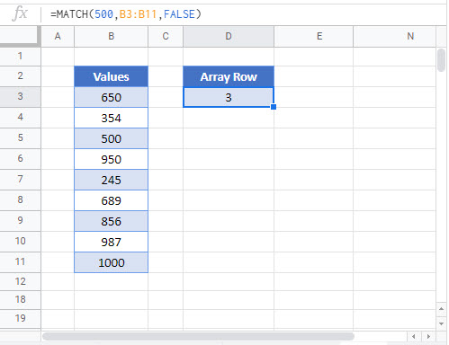
The MATCH Function is useful when you want to find a number within a array of values.
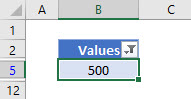
This example will find 500 in column B.
=MATCH(500,B3:B11, 0)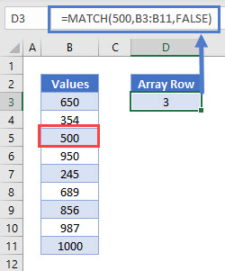
The position of 500 is the 3rd value in the range and returns 3.
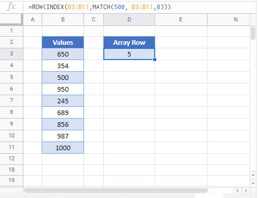
Find Row Number of Value Using ROW, INDEX and MATCH Functions
To find the row number of the value found, we can add the ROW and INDEX functions to the MATCH Function.
=ROW(INDEX(B3:B11,MATCH(987,B3:B11,0)))
ROW and INDEX Functions
The MATCH Function returns 3 as we have seen from the previous example. The INDEX Function will then return the cell reference or value of the array position returned by the MATCH Function. The ROW function will then return the row of that cell reference.
Filter in Excel
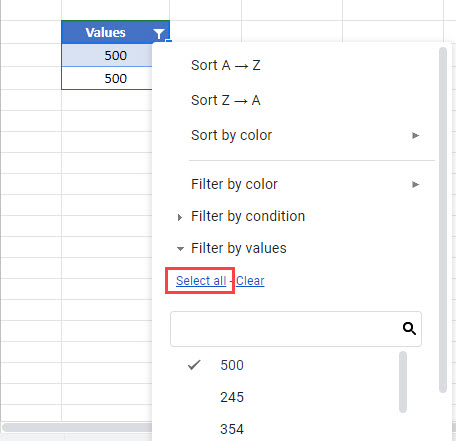
We can find a specific number in an array of data by using a Filter in Excel.
- Click in the Range you want to filter ex B3:B10.
- In the Ribbon, select Home > Editing > Sort & Filter > Filter.
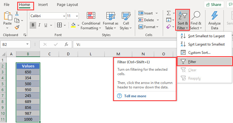
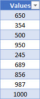
- A drop-down list will be added to the first row in your selected range.
- Click on the drop-down list to get a list of available options.
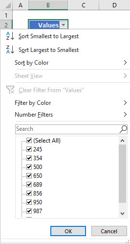
- Type 500 in the search bar.
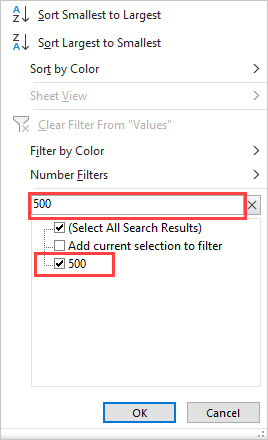
- Click OK.
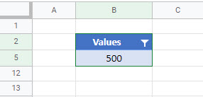
- If your range has more than one value of 500, then both would show.
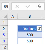
- The rows that do not contain the required values are hidden, and the visible row headers are shown in BLUE.
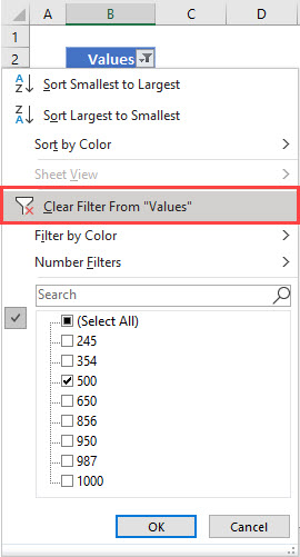
- To clear the filter, click on the drop-down and then click Clear Filter From “Values”.
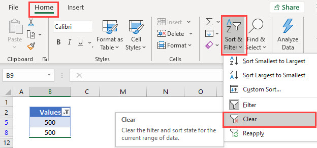
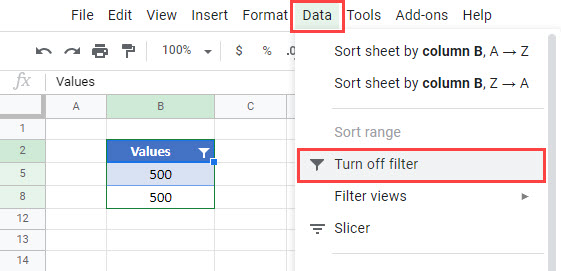
To remove the filter entirely from the Range, select Home > Editing > Sort & Filter > Clear in the Ribbon.
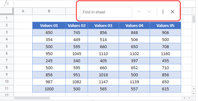
Find Number in Workbook or Worksheet using FIND in Excel
We can look for values in Excel using the FIND functionality.
- In your workbook, press Ctrl+F on the keyboard.
OR
In the Ribbon, select Home > Editing > Find & Select.
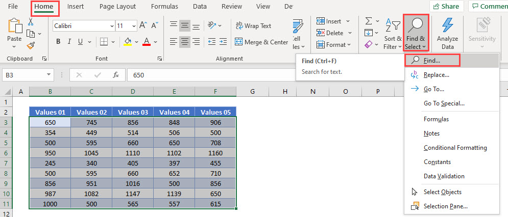
- Type in the value you wish to find.
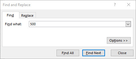
- Click Find Next.
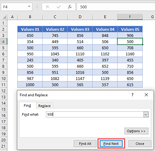
- Continue to click Find Next to move through all the available values in the Worksheet.
- Click Find All to find all the instances of the value in the worksheet.
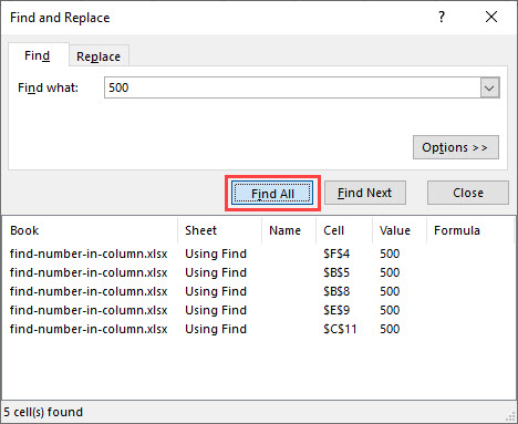
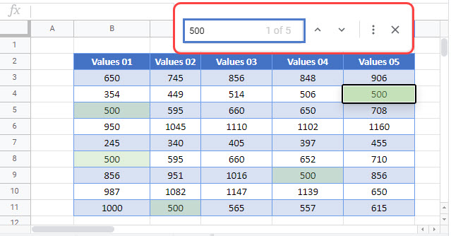
Click Options.
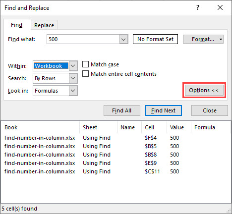
- Amend the Within from Sheet to Workbook and click Find All
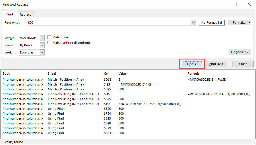
- All the matching values will appear in the results shown.
Find a Number – MATCH Function in Google Sheets
The MATCH Function works the same in Google Sheets as it does in Excel.
Find Row Number of Value Using ROW, INDEX and MATCH Functions in Google Sheets
The ROW, INDEX and MATCH Functions works the same in Google Sheets as it does in Excel.
Filter in Google Sheets
We can find a specific number in an array of data by using Filter in Google Sheets.
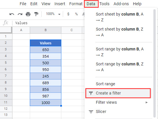
- Click in the Range you want to filter ex B3:B10.
- In the Menu, select Data > Create a filter
- In the Search bar, type in the value you wish to filter on.
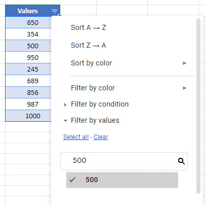
- Click OK.
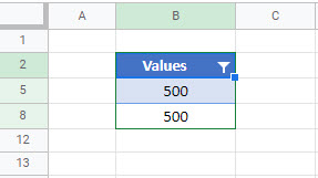
- If your range has more than one value of 500, then both would show.
- The rows that do not contain the required values are hidden.
- To clear the filter, click on the drop-down, click Select All” and then click
To remove the filter entire, in the Menu, select Data > Turn off Filter.
Find Number in Workbook or Worksheet using FIND in Google Sheets
We can look for values in Google Sheets using the FIND functionality.
- In your workbook, press Ctrl+F on the keyboard.
- Type in the value you wish to find.
- All the matching values in the current sheet will be highlighted, with the first one being selected as shown below.
- Select More Options.

- Amend the search to All Sheets.
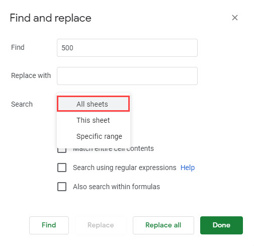
- Click Find.
- The first instance of the value will be found. Click Find again to go to the next value and continue to click Find to find all the matching values in the workbook.
- Click Done to exit out of the Find and Replace Dialog Box.
Содержание
- Метод Range.Find (Excel)
- Синтаксис
- Параметры
- Возвращаемое значение
- Примечания
- Примеры
- Поддержка и обратная связь
- VBA Find Value in Column
- Looping through a column with Range.Find and Range.FindNext
- VBA Coding Made Easy
- VBA Code Examples Add-in
- Find a Value in a Column Using Excel VBA
- Find a String/Value in a Column Using Find() Function in VBA
- Find a String/Value in a Column Using Match() Function in VBA
- Find a String/Value in a Column Using Loops in VBA
- Finding a String in Multiple Columns Using Loops in VBA
- VBA Excel. Метод Find объекта Range
- Предназначение и синтаксис метода Range.Find
- Синтаксис метода Range.Find
- Параметры метода Range.Find
- Знаки подстановки для поисковой фразы
- Простые примеры
Метод Range.Find (Excel)
Находит определенные сведения в диапазоне.
Хотите создавать решения, которые расширяют возможности Office на разнообразных платформах? Ознакомьтесь с новой моделью надстроек Office. Надстройки Office занимают меньше места по сравнению с надстройками и решениями VSTO, и вы можете создавать их, используя практически любую технологию веб-программирования, например HTML5, JavaScript, CSS3 и XML.
Синтаксис
выражение.Find (What, After, LookIn, LookAt, SearchOrder, SearchDirection, MatchCase, MatchByte, SearchFormat)
выражение: переменная, представляющая объект Range.
Параметры
| Имя | Обязательный или необязательный | Тип данных | Описание |
|---|---|---|---|
| What | Обязательный | Variant | Искомые данные. Может быть строкой или любым типом данных Microsoft Excel. |
| After | Необязательный | Variant | Ячейка, после которой нужно начать поиск. Соответствует положению активной ячейки, когда поиск выполняется из пользовательского интерфейса. |
Обратите внимание, что параметр After должен быть одной ячейкой в диапазоне. Помните, что поиск начинается после этой ячейки; указанная ячейка не входит в область поиска, пока метод не возвращается обратно в эту ячейку.
Если не указать этот аргумент, поиск начинается после ячейки в левом верхнем углу диапазона. LookIn Необязательный Variant Может быть одной из следующих констант XlFindLookIn: xlFormulas, xlValues, xlComments или xlCommentsThreaded. LookAt Необязательный Variant Может быть одной из следующих констант XlLookAt: xlWhole или xlPart. SearchOrder Необязательный Variant Может быть одной из следующих констант XlSearchOrder: xlByRows или xlByColumns. SearchDirection Необязательный Variant Может быть одной из следующих констант XlSearchDirection: xlNext или xlPrevious. MatchCase Необязательный Variant Значение True, чтобы выполнять поиск с учетом регистра. Значение по умолчанию — False. MatchByte Необязательный Variant Используется только в том случае, если выбрана или установлена поддержка двухбайтовых языков. Значение True, чтобы двухбайтовые символы сопоставлялись только с двухбайтовым символами. Значение False, чтобы двухбайтовые символы сопоставлялись с однобайтовыми эквивалентами. SearchFormat Необязательный Variant Формат поиска.
Возвращаемое значение
Объект Range, представляющий первую ячейку, в которой обнаружены требуемые сведения.
Примечания
Этот метод возвращает значение Nothing, если совпадения не найдены. Метод Find не влияет на выделенный фрагмент или активную ячейку.
Параметры для аргументов LookIn, LookAt, SearchOrder и MatchByte сохраняются при каждом использовании этого метода. Если не указать значения этих аргументов при следующем вызове метода, будут использоваться сохраненные значения. Установка этих аргументов изменяет параметры в диалоговом окне Найти, а изменение параметров в диалоговом окне Найти приводит к изменению сохраненных значений, которые используются, если опустить аргументы. Чтобы избежать проблем, устанавливайте эти аргументы явным образом при каждом использовании этого метода.
Для повторения поиска используйте методы FindNext и FindPrevious.
Когда поиск достигает конца указанного диапазона поиска, он возвращается в начало диапазона. Чтобы остановить поиск при этом возврате, сохраните адрес первой найденной ячейки, а затем проверьте адрес каждой последующей найденной ячейки, сравнив его с этим сохраненным адресом.
Чтобы найти ячейки, отвечающие более сложным шаблонам, используйте инструкцию For Each. Next с оператором Like. Например, следующий код выполняет поиск всех ячеек в диапазоне A1:C5, где используется шрифт, имя которого начинается с букв Cour. Когда Microsoft Excel находит соответствующее значение, шрифт изменяется на Times New Roman.
Примеры
В этом примере показано, как найти все ячейки в диапазоне A1:A500 на листе 1, содержащие значение 2, и изменить значение ячейки на 5. Таким образом, значения 1234 и 99299 содержали 2 и оба значения ячеек станут 5.
В этом примере показано, как найти все ячейки в диапазоне A1:A500 на листе 1, содержащие подстроку «abc», и изменить ее на «xyz».
Поддержка и обратная связь
Есть вопросы или отзывы, касающиеся Office VBA или этой статьи? Руководство по другим способам получения поддержки и отправки отзывов см. в статье Поддержка Office VBA и обратная связь.
Источник
VBA Find Value in Column
This article will demonstrate how to use VBA to find a value in a column.
We can use Range.Find to loop through a column of values in VBA to find all the cells in the range that match the criteria specified.
Looping through a column with Range.Find and Range.FindNext
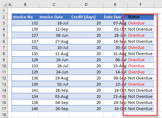
In the example below, we are looping through the data in the column, and looking for the word “Overdue”. When it finds the word, it will mark the cell by changing the color of the cell text to red. It will then us the Range.FindNext method to move onto the next cell and continue to look for the word, continuing the loop until the end of the specified range of cells.
When the code runs, it saves the address of the first cell where the data is found in the variable strFirstAddress and changes the color of the text to red. A loop is then created to find the next cell which contains the required data. When the value is found, the color of the text is changed to red and then the address of the cell where the value is found is compared to the string strFirstAddress. If these are not the same, the loop continues, finding each instance of the word “Overdue”. Once the loop reaches the end of the range of cells (ie F17), it will start back at the beginning of the range (F1) and continue to loop. Once it reaches the cell address F3 for the second time, as it is the same as the stored variable strFirstAddress, the loop will stop.
VBA Coding Made Easy
Stop searching for VBA code online. Learn more about AutoMacro — A VBA Code Builder that allows beginners to code procedures from scratch with minimal coding knowledge and with many time-saving features for all users! 

VBA Code Examples Add-in
Easily access all of the code examples found on our site.
Simply navigate to the menu, click, and the code will be inserted directly into your module. .xlam add-in.
Источник
Find a Value in a Column Using Excel VBA
Creating automation tools in Excel requires several string matching functions like Instr() , CStr() , Split() , etc. These functions find a substring within a string. However, when dealing with strings/values through column/s, you can’t use these functions as these are single-stringed functions.
This article will demonstrate three techniques for finding a string or a value in a column. The return value is the row number where the target string is.
String Search Techniques:
- Using Find() function
- Using Match function
- Using Loops
For the whole article, this virtual sheet will be the reference sheet.
Find a String/Value in a Column Using Find() Function in VBA
Parameters:
| Range | Required. Range object where to look the value or string. |
| What | Required. The string to search. |
| After | Optional. The cell after which you’d like the search to start. |
| LookIn | Optional. It could be xlFormulas , xlValues . |
| LookAt | Optional. It could be xlPart or xlWhole . |
| SearchOrder | Optional. It could be xlByRows or xlByColumns . |
| SearchDirection | Optional. It could be xlNext or xlPrevious |
| MatchCase | Optional. If the search is case sensitive, then True else False . |
The code block below will demonstrate using the Find() function to return the row of the string to search.
Find a String/Value in a Column Using Match() Function in VBA
The main difference between the Find() and Match() functions is that the former returns the Range object where the string is found while the latter returns the position where the string has a match.
Parameters:
| [StringtoSearch] | Required. String to look for |
| [RangetoSearchIn] | Required. Range object where to look the value or string |
| [MatchType] | Optional. Excel Matching Type. Refer to Remarks for Details |
For [MatchType] arguments, here are the values:
| 1 | finds the biggest value that is less than or equal to StringtoSearch |
| 0 | finds the exact StringtoSearch |
| -1 | finds the least value that is greater than or equal to StringtoSearch |
The code block below will demonstrate using the Match() function to return the row of the string to search.
Find a String/Value in a Column Using Loops in VBA
Unlike Find() and Match() functions, utilizing loops allows the user to execute the code. One advantage of loops is that we can return all the matches from a Range. However, loops are not recommended when dealing with large data as it is iterating with each cell within the specified limits.
The code block below will demonstrate utilizing loops to return the row of the string to search.
Finding a String in Multiple Columns Using Loops in VBA
The three code blocks above were designed to look into just one column. Rarely, you need to look for string matches across multiple columns or even within the whole worksheet. But if you need to, the code block below will help you.
Источник
VBA Excel. Метод Find объекта Range
Метод Find объекта Range для поиска ячейки по ее данным в VBA Excel. Синтаксис и компоненты. Знаки подстановки для поисковой фразы. Простые примеры.
Предназначение и синтаксис метода Range.Find
Метод Find объекта Range предназначен для поиска ячейки и сведений о ней в заданном диапазоне по ее значению, формуле и примечанию. Чаще всего этот метод используется для поиска в таблице ячейки по слову, части слова или фразе, входящей в ее значение.
Синтаксис метода Range.Find
Expression – это переменная или выражение, возвращающее объект Range, в котором будет осуществляться поиск.
В скобках перечислены параметры метода, среди них только What является обязательным.
Метод Range.Find возвращает объект Range, представляющий из себя первую ячейку, в которой найдена поисковая фраза (параметр What). Если совпадение не найдено, возвращается значение Nothing.
Если необходимо найти следующие ячейки, содержащие поисковую фразу, используется метод Range.FindNext.
Параметры метода Range.Find
| Наименование | Описание |
|---|---|
| Обязательный параметр | |
| What | Данные для поиска, которые могут быть представлены строкой или другим типом данных Excel. Тип данных параметра — Variant. |
| Необязательные параметры | |
| After | Ячейка, после которой следует начать поиск. |
| LookIn | Уточняет область поиска. Список констант xlFindLookIn:
|
| LookAt | Поиск частичного или полного совпадения. Список констант xlLookAt:
|
| SearchOrder | Определяет способ поиска. Список констант xlSearchOrder:
|
| SearchDirection | Определяет направление поиска. Список констант xlSearchDirection:
|
| MatchCase | Определяет учет регистра:
|
| MatchByte | Условия поиска при использовании двухбайтовых кодировок:
|
| SearchFormat | Формат поиска – используется вместе со свойством Application.FindFormat. |
* Примечания имеют две константы с одним значением. Проверяется очень просто: MsgBox xlComments и MsgBox xlNotes .
В справке Microsoft тип данных всех параметров, кроме SearchDirection, указан как Variant.
Знаки подстановки для поисковой фразы
Условные знаки в шаблоне поисковой фразы:
- ? – знак вопроса обозначает любой отдельный символ;
- * – звездочка обозначает любое количество любых символов, в том числе ноль символов;
Простые примеры
При использовании метода Range.Find в VBA Excel необходимо учитывать следующие нюансы:
- Так как этот метод возвращает объект Range (в виде одной ячейки), присвоить его можно только объектной переменной, объявленной как Variant, Object или Range, при помощи оператора Set.
- Если поисковая фраза в заданном диапазоне найдена не будет, метод Range.Find возвратит значение Nothing. Обращение к свойствам несуществующей ячейки будет генерировать ошибки. Поэтому, перед использованием результатов поиска, необходимо проверить объектную переменную на содержание в ней значения Nothing.
В примерах используются переменные:
- myPhrase – переменная для записи поисковой фразы;
- myCell – переменная, которой присваивается первая найденная ячейка, содержащая поисковую фразу, или значение Nothing, если поисковая фраза не найдена.
Источник
I have to find a value celda in an Excel sheet. I was using this vba code to find it:
Set cell = Cells.Find(What:=celda, After:=ActiveCell, LookIn:= _
    xlFormulas, LookAt:=xlWhole, SearchOrder:=xlByRows, SearchDirection:= _
    xlNext, MatchCase:=False, SearchFormat:=False)


If cell Is Nothing Then
    'do it something

Else
    'do it another thing
End If
The problem is when I have to find the value only in a excel column. I find it with next code:
    Columns("B:B").Select
    Selection.Find(What:="VA22GU1", After:=ActiveCell, LookIn:=xlFormulas, _
        LookAt:=xlWhole, SearchOrder:=xlByRows, SearchDirection:=xlNext, _
        MatchCase:=False, SearchFormat:=False).Activate
But I don’t know how to adapt it to the first vba code, because I have to use the value nothing.