Find the word in excel

SEARCH, SEARCHB functions

This article describes the formula syntax and usage of the SEARCH and SEARCHB functions in Microsoft Excel.

Description

The SEARCH and SEARCHB functions locate one text string within a second text string, and return the number of the starting position of the first text string from the first character of the second text string. For example, to find the position of the letter «n» in the word «printer», you can use the following function:

This function returns 4 because «n» is the fourth character in the word «printer.»

You can also search for words within other words. For example, the function

returns 5, because the word «base» begins at the fifth character of the word «database». You can use the SEARCH and SEARCHB functions to determine the location of a character or text string within another text string, and then use the MID and MIDB functions to return the text, or use the REPLACE and REPLACEB functions to change the text. These functions are demonstrated in Example 1 in this article.

These functions may not be available in all languages.

SEARCHB counts 2 bytes per character only when a DBCS language is set as the default language. Otherwise SEARCHB behaves the same as SEARCH, counting 1 byte per character.

The languages that support DBCS include Japanese, Chinese (Simplified), Chinese (Traditional), and Korean.

Syntax

The SEARCH and SEARCHB functions have the following arguments:

find_text Required. The text that you want to find.

within_text Required. The text in which you want to search for the value of the find_text argument.

start_num Optional. The character number in the within_text argument at which you want to start searching.

The SEARCH and SEARCHB functions are not case sensitive. If you want to do a case sensitive search, you can use FIND and FINDB.

You can use the wildcard characters — the question mark ( ?) and asterisk ( *) — in the find_text argument. A question mark matches any single character; an asterisk matches any sequence of characters. If you want to find an actual question mark or asterisk, type a tilde (

) before the character.

If the value of find_text is not found, the #VALUE! error value is returned.

If the start_num argument is omitted, it is assumed to be 1.

If start_num is not greater than 0 (zero) or is greater than the length of the within_text argument, the #VALUE! error value is returned.

Use start_num to skip a specified number of characters. Using the SEARCH function as an example, suppose you are working with the text string «AYF0093.YoungMensApparel». To find the position of the first «Y» in the descriptive part of the text string, set start_num equal to 8 so that the serial number portion of the text (in this case, «AYF0093») is not searched. The SEARCH function starts the search operation at the eighth character position, finds the character that is specified in the find_text argument at the next position, and returns the number 9. The SEARCH function always returns the number of characters from the start of the within_text argument, counting the characters you skip if the start_num argument is greater than 1.

Examples

Copy the example data in the following table, and paste it in cell A1 of a new Excel worksheet. For formulas to show results, select them, press F2, and then press Enter. If you need to, you can adjust the column widths to see all the data.

Источник

Find or replace text and numbers on a worksheet

Use the Find and Replace features in Excel to search for something in your workbook, such as a particular number or text string. You can either locate the search item for reference, or you can replace it with something else. You can include wildcard characters such as question marks, tildes, and asterisks, or numbers in your search terms. You can search by rows and columns, search within comments or values, and search within worksheets or entire workbooks.

Tip: You can also use formulas to replace text. Check out the SUBSTITUTE function or REPLACE, REPLACEB functions to learn more.

To find something, press Ctrl+F, or go to Home > Editing > Find & Select > Find.

Note: In the following example, we’ve clicked the Options >> button to show the entire Find dialog. By default, it will display with Options hidden.

In the Find what: box, type the text or numbers you want to find, or click the arrow in the Find what: box, and then select a recent search item from the list.

Tips: You can use wildcard characters — question mark ( ?), asterisk ( *), tilde (

) — in your search criteria.

Use the question mark (?) to find any single character — for example, s?t finds «sat» and «set».

Use the asterisk (*) to find any number of characters — for example, s*d finds «sad» and «started».

) followed by ?, *, or

to find question marks, asterisks, or other tilde characters — for example, fy91

Click Find All or Find Next to run your search.

Tip: When you click Find All, every occurrence of the criteria that you are searching for will be listed, and clicking a specific occurrence in the list will select its cell. You can sort the results of a Find All search by clicking a column heading.

Click Options>> to further define your search if needed:

Within: To search for data in a worksheet or in an entire workbook, select Sheet or Workbook.

Search: You can choose to search either By Rows (default), or By Columns.

Look in: To search for data with specific details, in the box, click Formulas, Values, Notes, or Comments.

Note: Formulas, Values, Notes and Comments are only available on the Find tab; only Formulas are available on the Replace tab.

Match case — Check this if you want to search for case-sensitive data.

Match entire cell contents — Check this if you want to search for cells that contain just the characters that you typed in the Find what: box.

If you want to search for text or numbers with specific formatting, click Format, and then make your selections in the Find Format dialog box.

Tip: If you want to find cells that just match a specific format, you can delete any criteria in the Find what box, and then select a specific cell format as an example. Click the arrow next to Format, click Choose Format From Cell, and then click the cell that has the formatting that you want to search for.

Replace

To replace text or numbers, press Ctrl+H, or go to Home > Editing > Find & Select > Replace.

Note: In the following example, we’ve clicked the Options >> button to show the entire Find dialog. By default, it will display with Options hidden.

In the Find what: box, type the text or numbers you want to find, or click the arrow in the Find what: box, and then select a recent search item from the list.

Tips: You can use wildcard characters — question mark ( ?), asterisk ( *), tilde (

) — in your search criteria.

Use the question mark (?) to find any single character — for example, s?t finds «sat» and «set».

Use the asterisk (*) to find any number of characters — for example, s*d finds «sad» and «started».

) followed by ?, *, or

to find question marks, asterisks, or other tilde characters — for example, fy91

In the Replace with: box, enter the text or numbers you want to use to replace the search text.

Click Replace All or Replace.

Tip: When you click Replace All, every occurrence of the criteria that you are searching for will be replaced, while Replace will update one occurrence at a time.

Click Options>> to further define your search if needed:

Within: To search for data in a worksheet or in an entire workbook, select Sheet or Workbook.

Search: You can choose to search either By Rows (default), or By Columns.

Look in: To search for data with specific details, in the box, click Formulas, Values, Notes, or Comments.

Note: Formulas, Values, Notes and Comments are only available on the Find tab; only Formulas are available on the Replace tab.

Match case — Check this if you want to search for case-sensitive data.

Match entire cell contents — Check this if you want to search for cells that contain just the characters that you typed in the Find what: box.

If you want to search for text or numbers with specific formatting, click Format, and then make your selections in the Find Format dialog box.

Tip: If you want to find cells that just match a specific format, you can delete any criteria in the Find what box, and then select a specific cell format as an example. Click the arrow next to Format, click Choose Format From Cell, and then click the cell that has the formatting that you want to search for.

There are two distinct methods for finding or replacing text or numbers on the Mac. The first is to use the Find & Replace dialog. The second is to use the Search bar in the ribbon.

Источник

Search For Text in Excel

How to Search For Text in Excel?

When working with Excel, we see so many peculiar situations. One of those situations is searching for the particular text in the cell. The first thing that comes to mind when we say we want to search for a specific text in the worksheet is the “Find and Replace” method in Excel, which is the most popular one. But Ctrl + F can find the text you are looking for but cannot go beyond that. So, for example, if the cell contains certain words, you may want the result in the next cell as “TRUE” or “FALSE.” So, Ctrl + F stops there.

Table of contents

You are free to use this image on your website, templates, etc., Please provide us with an attribution link How to Provide Attribution? Article Link to be Hyperlinked
For eg:
Source: Search For Text in Excel (wallstreetmojo.com)

Here, we will take you through the formulas to search for the particular text in the cell value and arrive at the result.

Which Formula Can Tell Us A Cell Contains Specific Text?

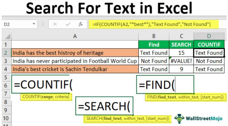
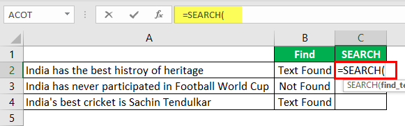
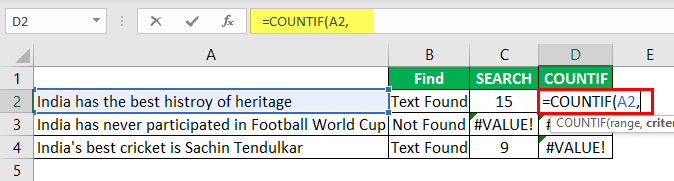
It is a question we have seen many times in Excel forums. The first formula that came to mind was the “FIND” function.

The FIND function can return the position of the supplied text values in the string. So, if the FIND method returns any number, then we can consider the cell as it has the text or else not.

1. For example, look at the below data.

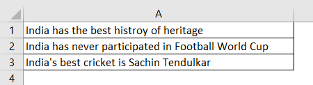
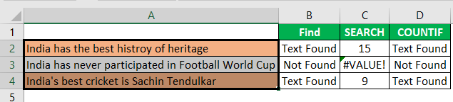
In the above data, we have three sentences in three different rows. Now in each cell, we need to search for the text “Best.” So, apply the FIND function.

The “find_text” argument mentions the text we need to find.

For the “within_text,” select the full sentence, i.e., cell reference.

The last parameter is not required to close the bracket and press the “Enter” key.

So, in two sentences, we have the word “best.” We can see the error value of #VALUE! in cell B2, which shows that cell A2 does not have the text value “best.”

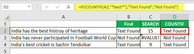
Instead of numbers, we can also enter the result in our own words. For this, we need to use the IF condition.

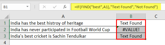
So, in the IF condition, we have supplied the result as “Text Found” if the value “best” is found. Otherwise, we have provided the result as “Not Found.”

But, here we have a problem, even though we have supplied the result as “Not Found,” if the text is still not found, we are getting the error value as #VALUE!.

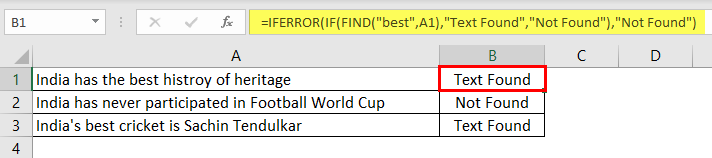
So, nobody wants to have an error value in their Excel sheet. Therefore, we must enclose the formula with the ISNUMERIC function to overcome this error value.

The ISNUMERIC function evaluates whether the FIND function returns the number or not. If the FIND function returns the number, it will supply TRUE to the IF condition or else FALSE condition. Based on the result provided by the ISNUMERIC function, the IF condition will return the result accordingly.

We can also use the IFERROR function in excel IFERROR Function In Excel The IFERROR function in Excel checks a formula (or a cell) for errors and returns a specified value in place of the error. read more to deal with error values instead of ISNUMERIC. For example, the below formula will also return “Not Found” if the FIND function returns the error value.

Alternatives to FIND Function

Alternative #1 – Excel Search Function

Supply the “find_text” as “Best.”

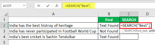
The “within_text” is our cell reference.

Even the SEARCH function returns an error value as #VALUE! If the finding text “best” is not found. As we have seen above, we need to enclose the formula with ISNUMERIC or IFERROR functions.

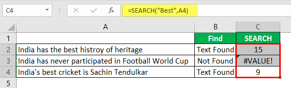
Alternative #2 – Excel Countif Function

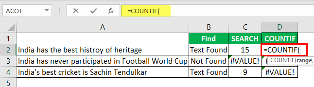
In the range, the argument selects the cell reference.

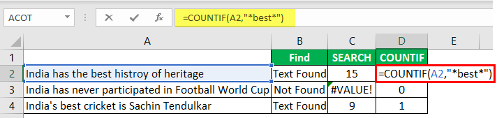
This formula will return the word “best” count in the selected cell value. Since we have only one “best” value, we will get only 1 as the count.

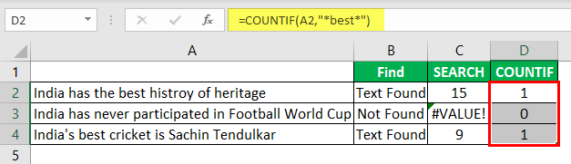
We can apply only the IF condition to get the result without error.

Highlight the Cell which has a Particular Text Value

First, select the data cells and click “Conditional Formatting” > “New Rule.”

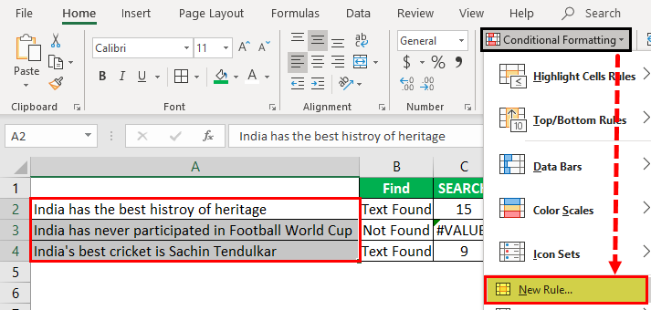
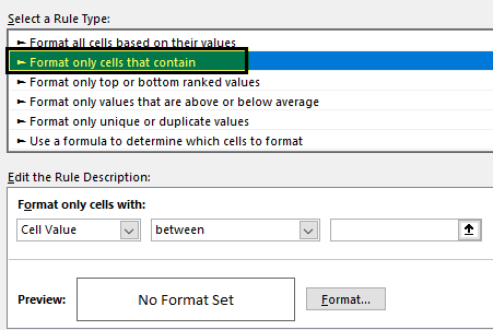
Under “New Rule,” select the “Format only cells that contain” option.

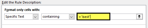
From the first dropdown, select “Specific Text.”

The formula section enters the text we search for in double quotes with the equal sign. =’best.’

Then, click on “FORMAT” and choose the formatting style.

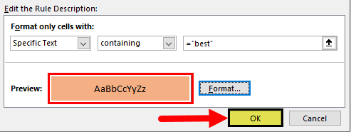
Click on “OK.” It will highlight all the cells which have the word “best.”

Using various techniques, we can search the particular text in Excel.

Recommended Articles

This article is a guide to Search For Text in Excel. Here, we discuss the top three methods to search the cell value for a specific text and arrive at the result with practical examples and a downloadable Excel template. You may learn more about Excel from the following articles: –

Источник