
Содержание
- Excel — find cell with same value in another worksheet and enter the value to the left of it [duplicate]
- 2 Answers 2
- How to use Cross-Sheet Operations
- Video: How to use Cross-Sheet Operations
- Start Cross-Sheet Operations
- Edit same cell across open workbooks
- Edit same cells in all open workbooks or only in the selected ones
- Undo one cell entry or edits to all cells
- Copy same cell or range values
- How to extract data
- How to reference same cells
- How to pull formulas from same cells
- Aggregate same cells and ranges
- How to sum same cells
- How to aggregate all same ranges together
- How to sum each range separately
- Related links
- 3-D reference in Excel: reference the same cell or range in multiple worksheets
- What is a 3D reference in Excel?
- How to create a 3-D reference in Excel
- How to include a new sheet in an Excel 3D formula
- How to create a name for an Excel 3-D reference
- Excel functions supporting 3-D references
- How Excel 3-D references change when you insert, move or delete sheets
Excel — find cell with same value in another worksheet and enter the value to the left of it [duplicate]
I have a report that is generated in Excel which contains an employee’s number, but not his/her name. Not every employee will be on this worksheet on any given day.
In a 2nd worksheet I have a list of all employees’ numbers and names.
I want a formula in the first worksheet that looks for the same value (the employee number) on the 2nd workbook and then enters the value of the cell to the RIGHT of that (the employee’s name) on the first workbook. Is there a way to do this? Thanks!
2 Answers 2
The easiest way is probably with VLOOKUP() . This will require the 2nd worksheet to have the employee number column sorted though. In newer versions of Excel, apparently sorting is no longer required.
For example, if you had a «Sheet2» with two columns — A = the employee number, B = the employee’s name, and your current worksheet had employee numbers in column D and you want to fill in column E, in cell E2, you would have:
Then simply fill this formula down the rest of column D.
- The first argument $D2 specifies the value to search for.
- The second argument Sheet2!$A$2:$B$65535 specifies the range of cells to search in. Excel will search for the value in the first column of this range (in this case Sheet2!A2:A65535 ). Note I am assuming you have a header cell in row 1.
- The third argument 2 specifies a 1-based index of the column to return from within the searched range. The value of 2 will return the second column in the range Sheet2!$A$2:$B$65535 , namely the value of the B column.
- The fourth argument FALSE says to only return exact matches.
Источник
How to use Cross-Sheet Operations
Cross-Sheet Operations helps to sum, copy, and reference the same cell or range across multiple Excel sheets. You can paste the values vertically or horizontally, aggregate your data, and edit same cell values in one window. Use the Cross-Sheet Range Operations tool to work with the same range or Cross-Sheet Cell Operations to edit and sum the same cell.
Video: How to use Cross-Sheet Operations
Start Cross-Sheet Operations
Open the Excel workbooks you want to work with and click Cross-Sheet Operations on the Ablebits Tools tab:
- To work with same cells, run Cross-Sheet Cell Operations.
- To perform operations with same ranges, click Cross-Sheet Range Operations.
The cell or range address is displayed at the top in the add-in pane:
To perform cross-sheet cell and range operations, use the tool’s elements:
- The tool remembers the cells and ranges you select. You can use these buttons to move to the previous or to the next selected cell.
- Click Paste Vertically if your task is to paste values from the same cell or range in a column. Then choose the paste options:
You can select to paste values, pull formulas, paste links to create references, or insert without borders.
Once the paste option is selected, choose the location for cell values:
You can either type the cell address into the field or select it in your worksheet.
- If you are working with Cell Operations, click this button to aggregate the same cell and paste only the result value. Select the function you need:
- When dealing with Range Operations, click this button to aggregate the same range and paste only the result values without formulas. Decide if you want to aggregate all ranges together or each range separately with the results pasted in a column or in a row. Hover over the chosen option and click on the function to perform:
Edit same cell across open workbooks
With the tool, you can edit the same cells in all open worksheets or only in the selected ones. You can undo one cell entry or all of them using special options.
Edit same cells in all open workbooks or only in the selected ones
- By default, all the open sheets are selected in the tool pane. Clear the checkboxes next to the worksheets which you don’t want to edit. To quickly select or deselect all worksheets in a workbook, select or clear the checkbox next to the workbook’s name:
- In the add-in pane, double-click a value next to any selected sheet, enter the value you need, and press the Enter key.
You will get the same values inserted into the same cell in all selected worksheets:
Undo one cell entry or edits to all cells
Once you edit a cell, two new buttons in the tool pane will appear. These are the Undo buttons:
- To undo one cell entry, click the Undo button next to the value:
- To undo edits in all sheets, click the Undo button on the add-in toolbar:
Copy same cell or range values
The tool provides several opportunities to copy the same cell or range values from multiple Excel worksheets. You can extract data, create references to the same cells, or pull formulas.
The first steps are the same as above:
- Open all worksheets that contain the cell or the range you need.
- In any of the opened worksheets, select the cell or the range you want to copy values from.
- Click Cross-Sheet Operations on the Ablebits Tools tab and select the option you need:
- In the add-in pane, make sure that all the sheets you are going to work with are selected.
- Decide if you want the values to be pasted in a row or in a column and click the corresponding button:
- Click Paste vertically to have your values organized in a column:
- Or Paste horizontally to have them in a row:
- To simply copy the same cell or range values, click the first paste option:
- Enter the cell address into the field in the dialogue window or select it in your worksheet:
How to reference same cells
- To create references to the same cell from multiple worksheets, click the Paste Link option:
- And then either enter the cell address into the field in the dialog window or select the cell in your worksheet.
How to pull formulas from same cells
To pull formulas from the same cells across several sheets, click the Paste Formulas option and then select where to place the result:
Aggregate same cells and ranges
The tool lets you apply a function to same cells and ranges in multiple Excel sheets. Run the Cross-Sheet Cell Operations tool to work with same cells or Cross-Sheet Range Operations to aggregate same ranges.
Decide if you want to paste the result value or the formula:
- If you need values only, click the Paste Values button:
- To insert formulas, click Paste Formulas:
How to sum same cells
- In the dropdown menu, click the function of interest:
- Then pick a cell to insert the result into and click OK:
How to aggregate all same ranges together
- To aggregate all same ranges, hover over the Paste the Result to One Cell option and select the function:
- In the dialog window that appears, pick a cell to paste the result value or formula and click OK.
How to sum each range separately
- To perform an operation with each same range separately, select to paste the result in a row or in a column, hover over the chosen option, and pick the function to apply:
- In the dialog window that appears, select the top left cell to paste the results and click OK.
Ultimate Suite for Excel
This tool is part of Ablebits Ultimate Suite that includes 70+ professional tools and 300+ solutions for daily tasks.
Table of contents
Is there a way to have a formula look for the same values in multiple worksheets and display them along a row. I’ve used the cross sheet function to pull values but need it to look up a value (like a H Lookup across the worksheets or a sumif). I do have the Ablebits ultimate suite.
Thank you for your comment. If you need to find the same value across multiple worksheets, then our Advanced Find and Replace can help. Yet, if you need a special formula, please visit our blog. You can ask your question in the Comments section under the corresponding topic and our tech specialist will do his best to help you out. Thank you.
Seen by everyone, do not publish license keys and sensitive personal info!
Источник
3-D reference in Excel: reference the same cell or range in multiple worksheets
 by Svetlana Cheusheva, updated on February 7, 2023
This short tutorial explains what Excel 3-D reference is and how you can use it to reference the same cell or a range of cells in all selected sheets. You will also learn how to make a 3-D formula to aggregate data in different worksheets, for example sum the same cell from multiple sheets with a single formula.
One of Excel’s greatest cell reference features is a 3D reference, or dimensional reference as it is also known.
A 3D reference in Excel refers to the same cell or range of cells on multiple worksheets. It is a very convenient and fast way to calculate data across several worksheets with the same structure, and it may be a good alternative to the Excel Consolidate feature. This may sound a bit vague, but don’t worry, the following examples will make things clearer.
What is a 3D reference in Excel?
As noted above, an Excel 3D reference lets you refer to the same cell or a range of cells in several worksheets. In other words, it references not only a range of cells, but also a range of worksheet names. The key point is that all of the referenced sheets should have the same pattern and the same data type. Please consider the following example.
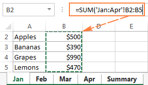
Supposing you have monthly sales reports in 4 different sheets: 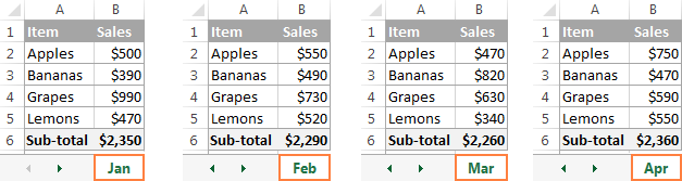
What you are looking for is finding out the grand total, i.e. adding up the sub-totals in four monthly sheets. The most obvious solution that comes to mind is add up the sub-total cells from all the worksheets in the usual way:
But what if you have 12 sheets for the whole year, or even more sheets for several years? This would be quite a lot of work. Instead, you can use the SUM function with a 3D reference to sum across sheets:
=SUM(Jan:Apr!B6)
This SUM formula performs the same calculations as the longer formula above, i.e. adds up the values in cell B6 in all the sheets between the two boundary worksheets that you specify, Jan and Apr in this example: 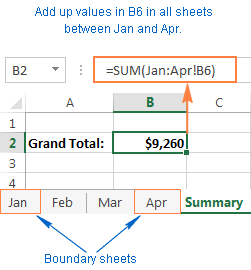
Tip. If you intend to copy your 3-D formula to several cells and you don’t want the cell references to change, you can lock them by adding the $ sign, i.e. by using absolute cells references like =SUM(Jan:Apr!$B$6) .
You don’t even need to calculate a sub-total in each monthly sheet — include the range of cells to be calculated directly in your 3D formula:
=SUM(Jan:Apr!B2:B5) 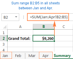
If you want to find out the sales total for each individual product, then make a summary table in which the items appear exactly in the same order as in monthly sheets, and input the following 3-D formula in the top-most cell, B2 in this example:
Remember to use a relative cell reference with no $ sign, so the formula gets adjusted for other cells when copied down the column: 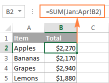
Based on the above examples, let’s make a generic Excel’s 3D reference and 3D formula.
Excel 3-D reference
Excel 3-D formula
When using such 3-D formulas in Excel, all worksheets between First_sheet and Last_sheet are included in calculations.
Note. Not all Excel functions support 3D references, here is the complete list of functions that do.
How to create a 3-D reference in Excel
To make a formula with a 3D reference, perform the following steps:
- Click the cell where you want to enter your 3D formula.
- Type the equal sign (=), enter the function’s name, and type an opening parenthesis, e.g. =SUM(
- Click the tab of the first worksheet that you want to include in a 3D reference.
- While holding the Shift key, click the tab of the last worksheet to be included in your 3D reference.
- Select the cell or range of cells that you want to calculate.
- Type the rest of the formula as usual.
- Press the Enter key to complete your Excel 3-D formula.
How to include a new sheet in an Excel 3D formula
3D references in Excel are extendable. What it means is that you can create a 3-D reference at some point, then insert a new worksheet, and move it into the range that your 3-D formula refers to. The following example provides full details.
Supposing it’s only the beginning of the year and you have data for the first few months only. However, a new sheet is likely to be added each month and you’d want to have those new sheets included in your calculations as they are created.
For this, create an empty sheet, say Dec, and make it the last sheet in your 3D reference:
When a new sheet is inserted in a workbook, simply move it anywhere between Jan and Dec: 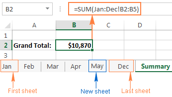
That’s it! Because your SUM formula contains a 3-D reference, it will add up the supplied range of cells (B2:B5) in all the worksheets within the specified range of worksheet names (Jan:Dec!). Just remember that all of the sheets included in an Excel 3D reference should have the same data layout and the same data type.
How to create a name for an Excel 3-D reference
To make it even easier for you to use 3D formulas in Excel, you can create a defined name for your 3D reference.
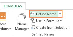
- On the Formulas tab, go to the Defined Names group and click Define Name.

- In the New Name dialog, type some meaningful and easy-to remember name in the Name box, up to 255 characters in length. In this example, let it be something very simple, say my_reference.
- Delete the contents of the Refers to box, and then enter a 3D reference there in the following way:
- Type = (equal sign).
- Hold down Shift, click the tab of the first sheet you want to reference, and then click the last sheet.
- Select the cell or range of cells to be referenced. You can also reference an entire column by clicking the column letter on the sheet.
In this example, let’s create an Excel 3D reference for the entire column B in sheets Jan through Apr. As the result, you’ll get something like this: 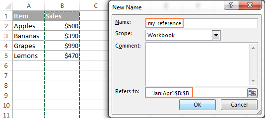
And now, to sum the numbers in column B in all the worksheets from Jan through Apr, you just use this simple formula:
=SUM(my_reference) 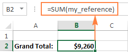
Excel functions supporting 3-D references
Here is a list of Excel functions that allow using 3-D references:
SUM — adds up numerical values.
AVERAGE — calculates arithmetic mean of numbers.
AVERAGEA — calculates arithmetic mean of values, including numbers, text and logicals.
COUNT — Counts cells with numbers.
COUNTA — Counts non-empty cells.
MAX — Returns the largest value.
MAXA — Returns the largest value, including text and logicals.
MIN — Finds the smallest value.
MINA — Finds the smallest value, including text and logicals.
PRODUCT — Multiplies numbers.
STDEV, STDEVA, STDEVP, STDEVPA — Calculate a sample deviation of a specified set of values.
VAR, VARA, VARP, VARPA — Returns a sample variance of a specified set of values.
How Excel 3-D references change when you insert, move or delete sheets
Because each 3D reference in Excel is defined by the starting and ending sheet, let’s call them the 3-D reference endpoints, changing the endpoints changes the reference, and consequently changes your 3D formula. And now, let’s see exactly what happens when you delete or move the 3-D reference endpoints, or insert, delete or move sheets within them.
Because nearly everything is easier to understand from an example, further explanations will be based on the following 3-D formula that we’ve created earlier: 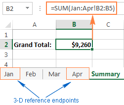
Insert, move or copy sheets within the endpoints. If you insert, copy or move worksheets between the 3D reference endpoints (Jan and Apr sheets in this example), the referenced range (cells B2 through B5) in all newly added sheets will be included in the calculations.
Delete sheets, or move sheets outside of the endpoints. When you delete any of the worksheets between the endpoints, or move sheets outside of the endpoints, such sheets are excluded from your 3D formula.
Move an endpoint. If you move either endpoint (Jan or Apr sheet, or both) to a new location within the same workbook, Excel will adjust your 3-D formula to include the new sheets that fall between the endpoints, and exclude those that have fallen out of the endpoints.
Reverse the endpoints. Reversing the Excel 3D reference endpoints results in changing one of the endpoint sheets. For example, if you move the starting sheet (Jan) after the ending sheet (Apr), the Jan sheet will be removed from the 3-D reference, which will change to Feb:Apr!B2:B5. 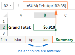
Moving the ending sheet (Apr) before the starting sheet (Jan) will have a similar effect. In this case, the Apr sheet will get excluded from the 3D reference that will change to Jan:Mar!B2:B5.
Please note that restoring the initial order of the endpoints won’t restore the original 3D reference. In the above example, even if we move the Jan sheet back to the first position, the 3D reference will remain Feb:Apr!B2:B5, and you will have to edit it manually to include Jan in your calculations.
Delete an endpoint. When you delete one of the endpoint sheets, it is removed from the 3D reference, and the deleted endpoint changes in the following way:
- If the first sheet is deleted, the endpoint changes to the sheet that follows it. In this example, if the Jan sheet is deleted, the 3D reference changes to Feb:Apr!B2:B5.
- If the last sheet is deleted, the endpoint changes to the preceding sheet. In this example, if the Apr sheet is deleted, the 3D reference changes to Jan:Mar!B2:B5.
This is how you create and use 3-D references in Excel. As you see, it’s a very convenient and fast way to calculate the same ranges in more than one sheet. While updating long formulas referencing different sheets might be tedious, an Excel 3-D formula requires updating just a couple of references, or you can simply insert new sheets between the 3D reference endpoints without changing the formula.
That’s all for today. I thank you for reading and hope to see you on our blog next week!
Источник
The easiest way is probably with VLOOKUP(). This will require the 2nd worksheet to have the employee number column sorted though. In newer versions of Excel, apparently sorting is no longer required.
For example, if you had a «Sheet2» with two columns — A = the employee number, B = the employee’s name, and your current worksheet had employee numbers in column D and you want to fill in column E, in cell E2, you would have:
=VLOOKUP($D2, Sheet2!$A$2:$B$65535, 2, FALSE)
Then simply fill this formula down the rest of column D.
Explanation:
- The first argument
$D2specifies the value to search for. - The second argument
Sheet2!$A$2:$B$65535specifies the range of cells to search in. Excel will search for the value in the first column of this range (in this caseSheet2!A2:A65535). Note I am assuming you have a header cell in row 1. - The third argument
2specifies a 1-based index of the column to return from within the searched range. The value of2will return the second column in the rangeSheet2!$A$2:$B$65535, namely the value of theBcolumn. - The fourth argument
FALSEsays to only return exact matches.
MATCH function
Tip: Try using the new XMATCH function, an improved version of MATCH that works in any direction and returns exact matches by default, making it easier and more convenient to use than its predecessor.
The MATCH function searches for a specified item in a range of cells, and then returns the relative position of that item in the range. For example, if the range A1:A3 contains the values 5, 25, and 38, then the formula =MATCH(25,A1:A3,0) returns the number 2, because 25 is the second item in the range.

Tip: Use MATCH instead of one of the LOOKUP functions when you need the position of an item in a range instead of the item itself. For example, you might use the MATCH function to provide a value for the row_num argument of the INDEX function.
Syntax
MATCH(lookup_value, lookup_array, [match_type])
The MATCH function syntax has the following arguments:
-
lookup_value Required. The value that you want to match in lookup_array. For example, when you look up someone’s number in a telephone book, you are using the person’s name as the lookup value, but the telephone number is the value you want.
The lookup_value argument can be a value (number, text, or logical value) or a cell reference to a number, text, or logical value.
-
lookup_array Required. The range of cells being searched.
-
match_type Optional. The number -1, 0, or 1. The match_type argument specifies how Excel matches lookup_value with values in lookup_array. The default value for this argument is 1.
The following table describes how the function finds values based on the setting of the match_type argument.
|
Match_type |
Behavior |
|
1 or omitted |
MATCH finds the largest value that is less than or equal to lookup_value. The values in the lookup_array argument must be placed in ascending order, for example: …-2, -1, 0, 1, 2, …, A-Z, FALSE, TRUE. |
|
0 |
MATCH finds the first value that is exactly equal to lookup_value. The values in the lookup_array argument can be in any order. |
|
-1 |
MATCH finds the smallest value that is greater than or equal tolookup_value. The values in the lookup_array argument must be placed in descending order, for example: TRUE, FALSE, Z-A, …2, 1, 0, -1, -2, …, and so on. |
-
MATCH returns the position of the matched value within lookup_array, not the value itself. For example, MATCH(«b»,{«a»,»b»,»c«},0) returns 2, which is the relative position of «b» within the array {«a»,»b»,»c»}.
-
MATCH does not distinguish between uppercase and lowercase letters when matching text values.
-
If MATCH is unsuccessful in finding a match, it returns the #N/A error value.
-
If match_type is 0 and lookup_value is a text string, you can use the wildcard characters — the question mark (?) and asterisk (*) — in the lookup_value argument. A question mark matches any single character; an asterisk matches any sequence of characters. If you want to find an actual question mark or asterisk, type a tilde (~) before the character.
Example
Copy the example data in the following table, and paste it in cell A1 of a new Excel worksheet. For formulas to show results, select them, press F2, and then press Enter. If you need to, you can adjust the column widths to see all the data.
|
Product |
Count |
|
|
Bananas |
25 |
|
|
Oranges |
38 |
|
|
Apples |
40 |
|
|
Pears |
41 |
|
|
Formula |
Description |
Result |
|
=MATCH(39,B2:B5,1) |
Because there is not an exact match, the position of the next lowest value (38) in the range B2:B5 is returned. |
2 |
|
=MATCH(41,B2:B5,0) |
The position of the value 41 in the range B2:B5. |
4 |
|
=MATCH(40,B2:B5,-1) |
Returns an error because the values in the range B2:B5 are not in descending order. |
#N/A |
Need more help?
Duplicate Values | Triplicates | Duplicate Rows
This example teaches you how to find duplicate values (or triplicates) and how to find duplicate rows in Excel.
Duplicate Values
To find and highlight duplicate values in Excel, execute the following steps.
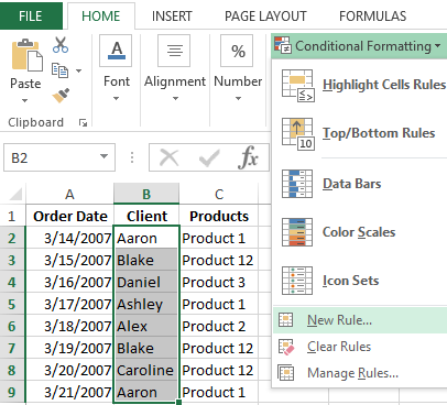
1. Select the range A1:C10.

2. On the Home tab, in the Styles group, click Conditional Formatting.

3. Click Highlight Cells Rules, Duplicate Values.

4. Select a formatting style and click OK.

Result. Excel highlights the duplicate names.

Note: select Unique from the first drop-down list to highlight the unique names.
Triplicates
By default, Excel highlights duplicates (Juliet, Delta), triplicates (Sierra), etc. (see previous image). Execute the following steps to highlight triplicates only.
1. First, clear the previous conditional formatting rule.
2. Select the range A1:C10.
3. On the Home tab, in the Styles group, click Conditional Formatting.
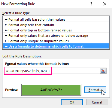
4. Click New Rule.

5. Select ‘Use a formula to determine which cells to format’.
6. Enter the formula =COUNTIF($A$1:$C$10,A1)=3
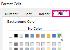
7. Select a formatting style and click OK.

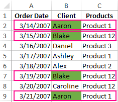
Result. Excel highlights the triplicate names.

Explanation: =COUNTIF($A$1:$C$10,A1) counts the number of names in the range A1:C10 that are equal to the name in cell A1. If COUNTIF($A$1:$C$10,A1) = 3, Excel formats cell A1. Always write the formula for the upper-left cell in the selected range (A1:C10). Excel automatically copies the formula to the other cells. Thus, cell A2 contains the formula =COUNTIF($A$1:$C$10,A2)=3, cell A3 =COUNTIF($A$1:$C$10,A3)=3, etc. Notice how we created an absolute reference ($A$1:$C$10) to fix this reference.
Note: you can use any formula you like. For example, use this formula =COUNTIF($A$1:$C$10,A1)>3 to highlight names that occur more than 3 times.
Duplicate Rows
To find and highlight duplicate rows in Excel, use COUNTIFS (with the letter S at the end) instead of COUNTIF.
1. Select the range A1:C10.

2. On the Home tab, in the Styles group, click Conditional Formatting.
3. Click New Rule.
4. Select ‘Use a formula to determine which cells to format’.
5. Enter the formula =COUNTIFS(Animals,$A1,Continents,$B1,Countries,$C1)>1
6. Select a formatting style and click OK.

Note: the named range Animals refers to the range A1:A10, the named range Continents refers to the range B1:B10 and the named range Countries refers to the range C1:C10. =COUNTIFS(Animals,$A1,Continents,$B1,Countries,$C1) counts the number of rows based on multiple criteria (Leopard, Africa, Zambia).
Result. Excel highlights the duplicate rows.

Explanation: if COUNTIFS(Animals,$A1,Continents,$B1,Countries,$C1) > 1, in other words, if there are multiple (Leopard, Africa, Zambia) rows, Excel formats cell A1. Always write the formula for the upper-left cell in the selected range (A1:C10). Excel automatically copies the formula to the other cells. We fixed the reference to each column by placing a $ symbol in front of the column letter ($A1, $B1 and $C1). As a result, cell A1, B1 and C1 contain the same formula, cell A2, B2 and C2 contain the formula =COUNTIFS(Animals,$A2,Continents,$B2,Countries,$C2)>1, etc.
7. Finally, you can use the Remove Duplicates tool in Excel to quickly remove duplicate rows. On the Data tab, in the Data Tools group, click Remove Duplicates.

In the example below, Excel removes all identical rows (blue) except for the first identical row found (yellow).


Note: visit our page about removing duplicates to learn more about this great Excel tool.
The searching of duplicates in Excel – is one of the most common tasks for any of office employee. For its solution, there are a few different methods. But – how quickly to find duplicates in Excel and to highlight them with color? For the answer on this frequently asked question let us consider a concrete example.
How to find duplicate values in Excel?
For example we are engaging by check orders, which coming into the firm through Fax and e-mail. There can be such situation that the same order was by the two channels of incoming information. If you register twice the same order, there can be certain problems for the firm. Below we are considering to the decision by means of the conditional formatting.
For avoiding of the duplicate orders, you can use to the conditional formatting, which helps you quickly to find the duplicate values in Excel column.
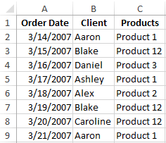
The example of the day orders for goods:
For verification whether the day orders are possible duplicates, we will analyze in the names of customers – there is the column B:
- To highlight the range B2:B9 and then to select the instrument: «HOME» — «Styles» — «Conditional Formatting» — «New Rule».
- To choose «Use a formula to determine which cells to format».
- To find the duplicate values in Excel column, you need to enter the formula in the input field:
- After that you need to press the button «Format» and select to the desired cell shading to highlight duplicates in color — for example, green one. And click OK on all windows are opened.
Download an example of finding the Identifying Duplicate values in a column.
As can be seen in the picture with the conditional formatting we were able easily and quickly to implement the duplicate finder in function Excel and to detect to the duplicate data cells for the table of the day orders.
The example of COUNTIF function and highlighting of the duplicate values
The principle of the action formula for finding of the duplicates by the conditional formatting is simple. The formula contains the function =COUNTIF(). This function can also be used when searching for the identical values in the range of cells. The first argument in the function to the viewable data range is specified. In the second argument we specify what we are looking for. The first argument has an absolute reference, as it should be the same one. And the second argument conversely — should be changed on the address of the each cell in the viewing range, because it has a relative link one.
The fastest and the simplest ways: to find to the duplicates in the cells.
After the function we can see the comparison operator of the number of the found values in the range with the number 1. That is, if we see more, than one value means that the formula returns the value of TRUE and for the current cell is applied to the conditional formatting.

Поиск какого-либо значения в ячейках Excel довольно часто встречающаяся задача при программировании какого-либо макроса. Решить ее можно разными способами. Однако, в разных ситуациях использование того или иного способа может быть не оправданным. В данной статье я рассмотрю 2 наиболее распространенных способа.
Поиск перебором значений
Довольно простой в реализации способ. Например, найти в колонке «A» ячейку, содержащую «123» можно примерно так:
Sheets("Данные").Select
For y = 1 To Cells.SpecialCells(xlLastCell).Row
    If Cells(y, 1) = "123" Then
        Exit For
    End If
Next y
MsgBox "Нашел в строке: " + CStr(y)
Минусами этого так сказать «классического» способа являются: медленная работа и громоздкость. А плюсом является его гибкость, т.к. таким способом можно реализовать сколь угодно сложные варианты поиска с различными вычислениями и т.п.
Поиск функцией Find
Гораздо быстрее обычного перебора и при этом довольно гибкий. В простейшем случае, чтобы найти в колонке A ячейку, содержащую «123» достаточно такого кода:
Sheets("Данные").Select
Set fcell = Columns("A:A").Find("123")
If Not fcell Is Nothing Then
    MsgBox "Нашел в строке: " + CStr(fcell.Row)
End If
Вкратце опишу что делают строчки данного кода:
1-я строка: Выбираем в книге лист «Данные»;
2-я строка: Осуществляем поиск значения «123» в колонке «A», результат поиска будет в fcell;
3-я строка: Если удалось найти значение, то fcell будет содержать Range-объект, в противном случае — будет пустой, т.е. Nothing.
Полностью синтаксис оператора поиска выглядит так:
Find(What, After, LookIn, LookAt, SearchOrder, SearchDirection, MatchCase, MatchByte, SearchFormat)
What — Строка с текстом, который ищем или любой другой тип данных Excel
After — Ячейка, после которой начать поиск. Обратите внимание, что это должна быть именно единичная ячейка, а не диапазон. Поиск начинается после этой ячейки, а не с нее. Поиск в этой ячейке произойдет только когда весь диапазон будет просмотрен и поиск начнется с начала диапазона и до этой ячейки включительно.
LookIn — Тип искомых данных. Может принимать одно из значений: xlFormulas (формулы), xlValues (значения), или xlNotes (примечания).
LookAt — Одно из значений: xlWhole (полное совпадение) или xlPart (частичное совпадение).
SearchOrder — Одно из значений: xlByRows (просматривать по строкам) или xlByColumns (просматривать по столбцам)
SearchDirection — Одно из значений: xlNext (поиск вперед) или xlPrevious (поиск назад)
MatchCase — Одно из значений: True (поиск чувствительный к регистру) или False (поиск без учета регистра)
MatchByte — Применяется при использовании мультибайтных кодировок: True (найденный мультибайтный символ должен соответствовать только мультибайтному символу) или False (найденный мультибайтный символ может соответствовать однобайтному символу)
SearchFormat — Используется вместе с FindFormat. Сначала задается значение FindFormat (например, для поиска ячеек с курсивным шрифтом так: Application.FindFormat.Font.Italic = True), а потом при использовании метода Find указываем параметр SearchFormat = True. Если при поиске не нужно учитывать формат ячеек, то нужно указать SearchFormat = False.
Чтобы продолжить поиск, можно использовать FindNext (искать «далее») или FindPrevious (искать «назад»).
Примеры поиска функцией Find
Пример 1: Найти в диапазоне «A1:A50» все ячейки с текстом «asd» и поменять их все на «qwe»
With Worksheets(1).Range("A1:A50")
  Set c = .Find("asd", LookIn:=xlValues)
  Do While Not c Is Nothing
    c.Value = "qwe"
    Set c = .FindNext(c)
  Loop
End With
Обратите внимание: Когда поиск достигнет конца диапазона, функция продолжит искать с начала диапазона. Таким образом, если значение найденной ячейки не менять, то приведенный выше пример зациклится в бесконечном цикле. Поэтому, чтобы этого избежать (зацикливания), можно сделать следующим образом:
Пример 2: Правильный поиск значения с использованием FindNext, не приводящий к зацикливанию.
With Worksheets(1).Range("A1:A50")
  Set c = .Find("asd", lookin:=xlValues)
  If Not c Is Nothing Then
    firstResult = c.Address
    Do
      c.Font.Bold = True
      Set c = .FindNext(c)
      If c Is Nothing Then Exit Do
    Loop While c.Address <> firstResult
  End If
End With
В ниже следующем примере используется другой вариант продолжения поиска — с помощью той же функции Find с параметром After. Когда найдена очередная ячейка, следующий поиск будет осуществляться уже после нее. Однако, как и с FindNext, когда будет достигнут конец диапазона, Find продолжит поиск с его начала, поэтому, чтобы не произошло зацикливания, необходимо проверять совпадение с первым результатом поиска.
Пример 3: Продолжение поиска с использованием Find с параметром After.
With Worksheets(1).Range("A1:A50")
  Set c = .Find("asd", lookin:=xlValues)
  If Not c Is Nothing Then
    firstResult = c.Address
    Do
      c.Font.Bold = True
      Set c = .Find("asd", After:=c, lookin:=xlValues)
      If c Is Nothing Then Exit Do
    Loop While c.Address <> firstResult
  End If
End With
Следующий пример демонстрирует применение SearchFormat для поиска по формату ячейки. Для указания формата необходимо задать свойство FindFormat.
Пример 4: Найти все ячейки с шрифтом «курсив» и поменять их формат на обычный (не «курсив»)
lLastRow = Cells.SpecialCells(xlLastCell).Row
lLastCol = Cells.SpecialCells(xlLastCell).Column
Application.FindFormat.Font.Italic = True
With Worksheets(1).Range(Cells(1, 1), Cells(lLastRow, lLastCol))
  Set c = .Find("", SearchFormat:=True)
  Do While Not c Is Nothing
    c.Font.Italic = False
    Set c = .Find("", After:=c, SearchFormat:=True)
  Loop
End With
Примечание: В данном примере намеренно не используется FindNext для поиска следующей ячейки, т.к. он не учитывает формат (статья об этом: https://support.microsoft.com/ru-ru/kb/282151)
Коротко опишу алгоритм поиска Примера 4. Первые две строки определяют последнюю строку (lLastRow) на листе и последний столбец (lLastCol). 3-я строка задает формат поиска, в данном случае, будем искать ячейки с шрифтом Italic. 4-я строка определяет область ячеек с которой будет работать программа (с ячейки A1 и до последней строки и последнего столбца). 5-я строка осуществляет поиск с использованием SearchFormat. 6-я строка — цикл пока результат поиска не будет пустым. 7-я строка — меняем шрифт на обычный (не курсив), 8-я строка продолжаем поиск после найденной ячейки.
Хочу обратить внимание на то, что в этом примере я не стал использовать «защиту от зацикливания», как в Примерах 2 и 3, т.к. шрифт меняется и после «прохождения» по всем ячейкам, больше не останется ни одной ячейки с курсивом.
Свойство FindFormat можно задавать разными способами, например, так:
With Application.FindFormat.Font
  .Name = "Arial"
  .FontStyle = "Regular"
  .Size = 10
End With
Поиск последней заполненной ячейки с помощью Find
Следующий пример — применение функции Find для поиска последней ячейки с заполненными данными. Использованные в Примере 4 SpecialCells находит последнюю ячейку даже если она не содержит ничего, но отформатирована или в ней раньше были данные, но были удалены.
Пример 5: Найти последнюю колонку и столбец, заполненные данными
Set c = Worksheets(1).UsedRange.Find("*", SearchDirection:=xlPrevious)
If Not c Is Nothing Then
  lLastRow = c.Row: lLastCol = c.Column
Else
  lLastRow = 1: lLastCol = 1
End If
MsgBox "lLastRow=" & lLastRow & " lLastCol=" & lLastCol
В этом примере используется UsedRange, который так же как и SpecialCells возвращает все используемые ячейки, в т.ч. и те, что были использованы ранее, а сейчас пустые. Функция Find ищет ячейку с любым значением с конца диапазона.
Поиск по шаблону (маске)
При поиске можно так же использовать шаблоны, чтобы найти текст по маске, следующий пример это демонстрирует.
Пример 6: Выделить красным шрифтом ячейки, в которых текст начинается со слова из 4-х букв, первая и последняя буквы «т», при этом после этого слова может следовать любой текст.
With Worksheets(1).Cells
  Set c = .Find("т??т*", LookIn:=xlValues, LookAt:=xlWhole)
  If Not c Is Nothing Then
    firstResult = c.Address
    Do
      c.Font.Color = RGB(255, 0, 0)
      Set c = .FindNext(c)
      If c Is Nothing Then Exit Do
    Loop While c.Address <> firstResult
  End If
End With
Для поиска функцией Find по маске (шаблону) можно применять символы:
* — для обозначения любого количества любых символов;
? — для обозначения одного любого символа;
~ — для обозначения символов *, ? и ~. (т.е. чтобы искать в тексте вопросительный знак, нужно написать ~?, чтобы искать именно звездочку (*), нужно написать ~* и наконец, чтобы найти в тексте тильду, необходимо написать ~~)
Поиск в скрытых строках и столбцах
Для поиска в скрытых ячейках нужно учитывать лишь один нюанс: поиск нужно осуществлять в формулах, а не в значениях, т.е. нужно использовать LookIn:=xlFormulas
Поиск даты с помощью Find
Если необходимо найти текущую дату или какую-то другую дату на листе Excel или в диапазоне с помощью Find, необходимо учитывать несколько нюансов:
- Тип данных Date в VBA представляется в виде #[месяц]/[день]/[год]#, соответственно, если необходимо найти фиксированную дату, например, 01 марта 2018 года, необходимо искать #3/1/2018#, а не «01.03.2018»
- В зависимости от формата ячеек, дата может выглядеть по-разному, поэтому, чтобы искать дату независимо от формата, поиск нужно делать не в значениях, а в формулах, т.е. использовать LookIn:=xlFormulas
Приведу несколько примеров поиска даты.
Пример 7: Найти текущую дату на листе независимо от формата отображения даты.
d = Date
Set c = Cells.Find(d, LookIn:=xlFormulas, LookAt:=xlWhole)
If Not c Is Nothing Then
  MsgBox "Нашел"
Else
  MsgBox "Не нашел"
End If
Пример 8: Найти 1 марта 2018 г.
d = #3/1/2018#
Set c = Cells.Find(d, LookIn:=xlFormulas, LookAt:=xlWhole)
If Not c Is Nothing Then
  MsgBox "Нашел"
Else
  MsgBox "Не нашел"
End If
Искать часть даты — сложнее. Например, чтобы найти все ячейки, где месяц «март», недостаточно искать «03» или «3». Не работает с датами так же и поиск по шаблону. Единственный вариант, который я нашел — это выбрать формат в котором месяц прописью для ячеек с датами и искать слово «март» в xlValues.
Тем не менее, можно найти, например, 1 марта независимо от года.
Пример 9: Найти 1 марта любого года.
d = #3/1/1900#
Set c = Cells.Find(Format(d, "m/d/"), LookIn:=xlFormulas, LookAt:=xlPart)
If Not c Is Nothing Then
  MsgBox "Нашел"
Else
  MsgBox "Не нашел"
End If