
Excel for Microsoft 365 Excel for Microsoft 365 for Mac Excel for the web Excel 2021 Excel 2021 for Mac Excel 2019 Excel 2019 for Mac Excel 2016 Excel 2016 for Mac Excel 2013 Excel 2010 Excel 2007 Excel for Mac 2011 Excel Starter 2010 More…Less
This article describes the formula syntax and usage of the FIND and FINDB functions in Microsoft Excel.
Description
FIND and FINDB locate one text string within a second text string, and return the number of the starting position of the first text string from the first character of the second text string.
Important:
-
These functions may not be available in all languages.
-
FIND is intended for use with languages that use the single-byte character set (SBCS), whereas FINDB is intended for use with languages that use the double-byte character set (DBCS). The default language setting on your computer affects the return value in the following way:
-
FIND always counts each character, whether single-byte or double-byte, as 1, no matter what the default language setting is.
-
FINDB counts each double-byte character as 2 when you have enabled the editing of a language that supports DBCS and then set it as the default language. Otherwise, FINDB counts each character as 1.
The languages that support DBCS include Japanese, Chinese (Simplified), Chinese (Traditional), and Korean.
Syntax
FIND(find_text, within_text, [start_num])
FINDB(find_text, within_text, [start_num])
The FIND and FINDB function syntax has the following arguments:
-
Find_text Required. The text you want to find.
-
Within_text Required. The text containing the text you want to find.
-
Start_num Optional. Specifies the character at which to start the search. The first character in within_text is character number 1. If you omit start_num, it is assumed to be 1.
Remarks
-
FIND and FINDB are case sensitive and don’t allow wildcard characters. If you don’t want to do a case sensitive search or use wildcard characters, you can use SEARCH and SEARCHB.
-
If find_text is «» (empty text), FIND matches the first character in the search string (that is, the character numbered start_num or 1).
-
Find_text cannot contain any wildcard characters.
-
If find_text does not appear in within_text, FIND and FINDB return the #VALUE! error value.
-
If start_num is not greater than zero, FIND and FINDB return the #VALUE! error value.
-
If start_num is greater than the length of within_text, FIND and FINDB return the #VALUE! error value.
-
Use start_num to skip a specified number of characters. Using FIND as an example, suppose you are working with the text string «AYF0093.YoungMensApparel». To find the number of the first «Y» in the descriptive part of the text string, set start_num equal to 8 so that the serial-number portion of the text is not searched. FIND begins with character 8, finds find_text at the next character, and returns the number 9. FIND always returns the number of characters from the start of within_text, counting the characters you skip if start_num is greater than 1.
Examples
Copy the example data in the following table, and paste it in cell A1 of a new Excel worksheet. For formulas to show results, select them, press F2, and then press Enter. If you need to, you can adjust the column widths to see all the data.
|
Data |
||
|
Miriam McGovern |
||
|
Formula |
Description |
Result |
|
=FIND(«M»,A2) |
Position of the first «M» in cell A2 |
1 |
|
=FIND(«m»,A2) |
Position of the first «M» in cell A2 |
6 |
|
=FIND(«M»,A2,3) |
Position of the first «M» in cell A2, starting with the third character |
8 |
Example 2
|
Data |
||
|
Ceramic Insulators #124-TD45-87 |
||
|
Copper Coils #12-671-6772 |
||
|
Variable Resistors #116010 |
||
|
Formula |
Description (Result) |
Result |
|
=MID(A2,1,FIND(» #»,A2,1)-1) |
Extracts text from position 1 to the position of «#» in cell A2 (Ceramic Insulators) |
Ceramic Insulators |
|
=MID(A3,1,FIND(» #»,A3,1)-1) |
Extracts text from position 1 to the position of «#» in cell A3 (Copper Coils) |
Copper Coils |
|
=MID(A4,1,FIND(» #»,A4,1)-1) |
Extracts text from position 1 to the position of «#» in cell A4 (Variable Resistors) |
Variable Resistors |
Need more help?
Содержание
- How to Find Cells containing Formulas in Excel
- Method 1: Using ‘Go To Special’ Option:
- Method 2: Using a built-in Excel formula
- Method 3: Using a Macro for identifying the cells that contain formulas:
- Subscribe and be a part of our 15,000+ member family!
- FIND, FINDB functions
- Description
- Syntax
- Remarks
- Examples
- Use Excel built-in functions to find data in a table or a range of cells
- Summary
- Create the Sample Worksheet
- Term Definitions
- Functions
- LOOKUP()
- VLOOKUP()
- INDEX() and MATCH()
- OFFSET() and MATCH()
- FIND Function
- Related functions
- Summary
- Purpose
- Return value
- Arguments
- Syntax
- Usage notes
- Basic Example
- Case-sensitive
- TRUE or FALSE result
- Start number
- Wildcards
- If cell contains
How to Find Cells containing Formulas in Excel
A few days back I had a huge spreadsheet in which I had to find out the cells containing formulas. Initially, I was totally clueless about how this task can be done.
But later after doing some Google searches, I got a few ideas on how I can effortlessly identify the formula cells in excel.
And today to share my experiences with you guys, In this post I will throw some light on a few methods that can help you to find out formula cells in your spreadsheets.
Method 1: Using ‘Go To Special’ Option:
In Excel ‘Go To Special’ is a very handy option when it comes to finding the cells with formulas. ‘Go to Special’ option has a radio button “Formulas” and selecting this radio button enables it to select all the cells containing formulas.
Later you can change the formatting or background color of the selected cells to make them stand out from the rest. Below is the step by step instructions for accomplishing this:
1. With your excel sheet opened navigate to the ‘Home’ tab > ‘Find & Select’ > ‘Go To Special’. Alternatively, you can also press ‘F5’ and then ‘Alt + S’ to open the ‘Go to Special’ dialog.

2. Next, in the ‘Go to Special’ window select the ‘Formulas’ radio button. After checking this radio button you will notice that few checkboxes (like Numbers, Errors, Logical, and Text) are enabled, these checkboxes signify the return type of the formulas.
So, if you select the ‘Formulas’ radio button and only check the ‘Numbers’ checkbox then it will just search the Formulas whose return type is a number. Here in our example, we will keep all of these return types checked.
3. After this click the ‘Ok’ button and all the cells that contain formulas get selected.
4. Next, without clicking anywhere on your spreadsheet change the background color of all the selected cells.
5. Now your formula cells can be easily identified.
Method 2: Using a built-in Excel formula
If you have worked with excel formulas then probably you may be knowing that excel has a formula that can find whether a cell contains a formula or not. The formula that I am talking about is:
Here ‘reference’ signifies the cell position which you wish to check for the presence of a formula.
For example: If you wish to check the cell ‘A2’ for the existence of a formula then you can use this function as
This function results in a Boolean output i.e. True or False. True signifies that the cell contains formulas while False tells that cell doesn’t contain any formulas.
Method 3: Using a Macro for identifying the cells that contain formulas:
I have created a VBA Macro that can find and color any cells that contain the formula in the total used range of the Active sheet. To use this macro simply follow the below procedure:
1. Open your spreadsheet and hit the ‘Alt + F11’ keys to open the VBA editor.

2. Next, navigate to ‘Insert‘ > ‘Module‘ and then paste the below macro in the editor.
3. For running this formula press the “F5” key.
4. This Macro will change the background colour of all the formula containing cells and thus makes it easier to identify them easily.
Subscribe and be a part of our 15,000+ member family!
Now subscribe to Excel Trick and get a free copy of our ebook «200+ Excel Shortcuts» (printable format) to catapult your productivity.
Источник
FIND, FINDB functions
This article describes the formula syntax and usage of the FIND and FINDB functions in Microsoft Excel.
Description
FIND and FINDB locate one text string within a second text string, and return the number of the starting position of the first text string from the first character of the second text string.
These functions may not be available in all languages.
FIND is intended for use with languages that use the single-byte character set (SBCS), whereas FINDB is intended for use with languages that use the double-byte character set (DBCS). The default language setting on your computer affects the return value in the following way:
FIND always counts each character, whether single-byte or double-byte, as 1, no matter what the default language setting is.
FINDB counts each double-byte character as 2 when you have enabled the editing of a language that supports DBCS and then set it as the default language. Otherwise, FINDB counts each character as 1.
The languages that support DBCS include Japanese, Chinese (Simplified), Chinese (Traditional), and Korean.
Syntax
FIND(find_text, within_text, [start_num])
FINDB(find_text, within_text, [start_num])
The FIND and FINDB function syntax has the following arguments:
Find_text Required. The text you want to find.
Within_text Required. The text containing the text you want to find.
Start_num Optional. Specifies the character at which to start the search. The first character in within_text is character number 1. If you omit start_num, it is assumed to be 1.
FIND and FINDB are case sensitive and don’t allow wildcard characters. If you don’t want to do a case sensitive search or use wildcard characters, you can use SEARCH and SEARCHB.
If find_text is «» (empty text), FIND matches the first character in the search string (that is, the character numbered start_num or 1).
Find_text cannot contain any wildcard characters.
If find_text does not appear in within_text, FIND and FINDB return the #VALUE! error value.
If start_num is not greater than zero, FIND and FINDB return the #VALUE! error value.
If start_num is greater than the length of within_text, FIND and FINDB return the #VALUE! error value.
Use start_num to skip a specified number of characters. Using FIND as an example, suppose you are working with the text string «AYF0093.YoungMensApparel». To find the number of the first «Y» in the descriptive part of the text string, set start_num equal to 8 so that the serial-number portion of the text is not searched. FIND begins with character 8, finds find_text at the next character, and returns the number 9. FIND always returns the number of characters from the start of within_text, counting the characters you skip if start_num is greater than 1.
Examples
Copy the example data in the following table, and paste it in cell A1 of a new Excel worksheet. For formulas to show results, select them, press F2, and then press Enter. If you need to, you can adjust the column widths to see all the data.
Источник
Use Excel built-in functions to find data in a table or a range of cells
Summary
This step-by-step article describes how to find data in a table (or range of cells) by using various built-in functions in Microsoft Excel. You can use different formulas to get the same result.
Create the Sample Worksheet
This article uses a sample worksheet to illustrate Excel built-in functions. Consider the example of referencing a name from column A and returning the age of that person from column C. To create this worksheet, enter the following data into a blank Excel worksheet.
You will type the value that you want to find into cell E2. You can type the formula in any blank cell in the same worksheet.
Term Definitions
This article uses the following terms to describe the Excel built-in functions:
The whole lookup table
The value to be found in the first column of Table_Array.
Lookup_Array
-or-
Lookup_Vector
The range of cells that contains possible lookup values.
The column number in Table_Array the matching value should be returned for.
3 (third column in Table_Array)
Result_Array
-or-
Result_Vector
A range that contains only one row or column. It must be the same size as Lookup_Array or Lookup_Vector.
A logical value (TRUE or FALSE). If TRUE or omitted, an approximate match is returned. If FALSE, it will look for an exact match.
This is the reference from which you want to base the offset. Top_Cell must refer to a cell or range of adjacent cells. Otherwise, OFFSET returns the #VALUE! error value.
This is the number of columns, to the left or right, that you want the upper-left cell of the result to refer to. For example, «5» as the Offset_Col argument specifies that the upper-left cell in the reference is five columns to the right of reference. Offset_Col can be positive (which means to the right of the starting reference) or negative (which means to the left of the starting reference).
Functions
LOOKUP()
The LOOKUP function finds a value in a single row or column and matches it with a value in the same position in a different row or column.
The following is an example of LOOKUP formula syntax:
The following formula finds Mary’s age in the sample worksheet:
The formula uses the value «Mary» in cell E2 and finds «Mary» in the lookup vector (column A). The formula then matches the value in the same row in the result vector (column C). Because «Mary» is in row 4, LOOKUP returns the value from row 4 in column C (22).
NOTE: The LOOKUP function requires that the table be sorted.
For more information about the LOOKUP function, click the following article number to view the article in the Microsoft Knowledge Base:
VLOOKUP()
The VLOOKUP or Vertical Lookup function is used when data is listed in columns. This function searches for a value in the left-most column and matches it with data in a specified column in the same row. You can use VLOOKUP to find data in a sorted or unsorted table. The following example uses a table with unsorted data.
The following is an example of VLOOKUP formula syntax:
The following formula finds Mary’s age in the sample worksheet:
The formula uses the value «Mary» in cell E2 and finds «Mary» in the left-most column (column A). The formula then matches the value in the same row in Column_Index. This example uses «3» as the Column_Index (column C). Because «Mary» is in row 4, VLOOKUP returns the value from row 4 in column C (22).
For more information about the VLOOKUP function, click the following article number to view the article in the Microsoft Knowledge Base:
INDEX() and MATCH()
You can use the INDEX and MATCH functions together to get the same results as using LOOKUP or VLOOKUP.
The following is an example of the syntax that combines INDEX and MATCH to produce the same results as LOOKUP and VLOOKUP in the previous examples:
The following formula finds Mary’s age in the sample worksheet:
The formula uses the value «Mary» in cell E2 and finds «Mary» in column A. It then matches the value in the same row in column C. Because «Mary» is in row 4, the formula returns the value from row 4 in column C (22).
NOTE: If none of the cells in Lookup_Array match Lookup_Value («Mary»), this formula will return #N/A.
For more information about the INDEX function, click the following article number to view the article in the Microsoft Knowledge Base:
OFFSET() and MATCH()
You can use the OFFSET and MATCH functions together to produce the same results as the functions in the previous example.
The following is an example of syntax that combines OFFSET and MATCH to produce the same results as LOOKUP and VLOOKUP:
This formula finds Mary’s age in the sample worksheet:
The formula uses the value «Mary» in cell E2 and finds «Mary» in column A. The formula then matches the value in the same row but two columns to the right (column C). Because «Mary» is in column A, the formula returns the value in row 4 in column C (22).
For more information about the OFFSET function, click the following article number to view the article in the Microsoft Knowledge Base:
Источник
FIND Function

Summary
The Excel FIND function returns the position (as a number) of one text string inside another. When the text is not found, FIND returns a #VALUE error.
Purpose
Return value
Arguments
- find_text — The substring to find.
- within_text — The text to search within.
- start_num — [optional] The starting position in the text to search. Optional, defaults to 1.
Syntax
Usage notes
The FIND function returns the position (as a number) of one text string inside another. If there is more than one occurrence of the search string, FIND returns the position of the first occurrence. When the text is not found, FIND returns a #VALUE error. Also note, when find_text is empty, FIND returns 1. FIND does not support wildcards, and is always case-sensitive. Use the SEARCH function to find the position of text without case-sensitivity and with wildcard support.
Basic Example
The FIND function is designed to look inside a text string for a specific substring. When FIND locates the substring, it returns a position of the substring in the text as a number. If the substring is not found, FIND returns a #VALUE error. For example:
Note that text values entered directly into FIND must be enclosed in double-quotes («»).
Case-sensitive
The FIND function always case-sensitive:
TRUE or FALSE result
To force a TRUE or FALSE result, nest the FIND function inside the ISNUMBER function. ISNUMBER returns TRUE for numeric values and FALSE for anything else. If FIND locates the substring, it returns the position as a number, and ISNUMBER returns TRUE:
If FIND doesn’t locate the substring, it returns an error, and ISNUMBER returns FALSE.
Start number
The FIND function has an optional argument called start_num, that controls where FIND should begin looking for a substring. To find the first match of «the» in any combination of upper or lowercase, you can omit start_num, which defaults to 1:
To start searching at character 5, enter 4 for start_num:
Wildcards
The FIND function does not support wildcards. See the SEARCH function.
If cell contains
To return a custom result with the SEARCH function, use the IF function like this:
Instead of returning TRUE or FALSE, the formula above will return «Yes» if substring is found and «No» if not.
Источник
In this video, we’re going to look at three ways to find formulas in a worksheet. Knowing where formulas are is the first step in understanding how a spreadsheet works.
When you first open a worksheet you didn’t create yourself, it may not be clear exactly where the formulas are.
Of course, you can just start selecting cells, while watching the formula bar, but there are several faster ways to find all formulas at once.
First, you can toggle the visibility of formulas on or off using the keyboard shortcut Control + Grave Accent. This key is just below the Escape key on US keyboards. This shortcut will cause Excel to display the formulas themselves instead of their results. Using this shortcut, you can quickly and easily switch back and forth.
The next way you can find all formulas is to use Go To Special. Go To Special is based on the Go To Dialog. The fastest way to open this dialog box is to use the keyboard shortcut Control-G. This works on both Windows and Mac platforms.
In the Go To dialog box, click Special, select Formulas, and then click OK. Excel will select all cells that contain formulas.
In the status bar, we can see the number of cells selected.
With all formulas selected, you can easily apply formatting. For example, let’s add a light yellow fill. Now all cells that contain formulas are marked for easy reference.
To clear this formatting. We can just reverse the process.
[go to special, clear formatting]
A third way to visually highlight formulas is to use Conditional Formatting. Excel 2013 includes a new formula called ISFORMULA(), which makes for a very simple Conditional Formatting rule, but that won’t work in older versions of Excel.
Instead, we’ll use a function called GET.CELL(), which is part of the XLM Macro language that preceded VBA. Unfortunately, GET.CELL can’t be used directly in a worksheet. However, by using a named formula, we can work around this problem.
First, we create a new name called CellHasFormula. For the reference, we use the GET.CELL function like so:
=GET.CELL(48,INDIRECT("rc",FALSE))
The first argument—48—tells GET.CELL to return TRUE if a cell contains a formula. The second parameter is the INDIRECT function. In this case, «rc» means current row and column, and FALSE tells INDIRECT that we are using R1C1 style references instead of A1 style references.
Now we can select the range we want to work with and create a new Conditional Formatting rule. We want to use a formula to control formatting, and the formula we use is simply our named formula «CellHasFormula.»
Once we set the format, we’ll see it applied to the cells that contain formulas. Because the highlighting is applied with Conditional Formatting, it’s fully dynamic. If we add a new formula, we’ll see it highlighted too.
One advantage to using Conditional Formatting is that the actual formatting of the cells is not affected. To stop highlighting formulas, simply delete the rule.
The next time you inherit a new workbook, try one of these 3 methods to quickly and easily find all formulas.
Three ways to find and highlight formulas:
1. Toggle Formulas with Control + `
2. Go To Special > Formulas
3. Conditional formatting with GET.CELL as named formula
The two formulas FIND and SEARCH in Excel are very similar. They search through a cell or some text for a keyword or character. Once found, they return the number of characters, at which the keyword starts. Let’s learn how to use them and explore the differences of the two formulas.
How to use the FIND formula
The formula returns the number of the character, at which your search term starts. If your text can’t be found, it’ll return a “#VALUE” error.
Structure of the FIND formula

The structure of the FIND formula is quite simple (the numbers are corresponding to the image on the right-hand side):
- SEARCH TERM: The first part of the formula is the text you look for.
- WITHIN TEXT: The cell or text you want to search your “SEARCH TERM” in.
- START NUMBER: This argument is optional. If you don’t want to start searching at the beginning of the text, fill in the number larger than 1, otherwise just type 1 or leave it blank.
If you just want to know, if your text can be found within another cell, you might want to go with the following formula. B2 contains the text or character you search for and B3 is the cell you search in:
=IFERROR(IF(FIND(B2,B3)>0,”Value found”,””),”Value not found”)
Please note the following comments:
- FIND is case-sensitive. That means, it matters if you use small or capital letters.
- You can also search for numbers within another number. For example: =FIND(1,321)This formula returns 3 because the number 1 is the third character of 321.
- You can’t use wildcard criteria (“*” or “?”) with the FIND formula.
- Please refer to this article if you want to know more about the IF formula and to this article for more information about the IFERROR formula.
Examples for the FIND formula
Let’s try some examples.
Example 1: Find the first occurrence
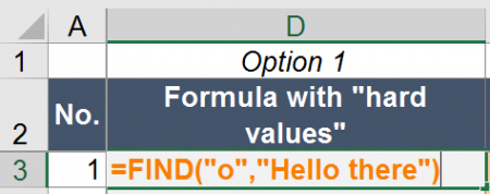
The “default” usage of the FIND formula is to return the number of characters, at which a text first occurs within another text. Let’s say you have the text “Hello there” and want to know, at which position you have an “o”. In such case, you write the following formula (example number 1 in the Excel workbook you can download at the end of this article).
=FIND(“o”,”Hello there”)
The return value is 5.
Example 2: Find the first occurrence after the third character
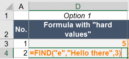
Another example: You want to know the position of “e” after the third character (example number 2 in the example workbook).
=FIND(“e”,”Hello there”,3)
The return value is 9.
Example 3: Find the second occurrence
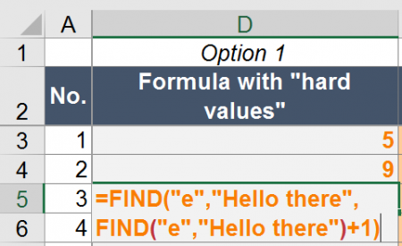
Now you want to know the position of the second occurrence of “e” in “Hello there”.
=FIND(“e”;”Hello there”;FIND(“e”;”Hello there”)+1)
This formula works as follows. The second FIND formula returns the position of the first occurrence of “e” in “Hello there” which is 2. This is used as the START NUMBER (+ 1 because you want to start counting after the first “e”) for the first FIND formula.
Example 4: Find the last occurrence
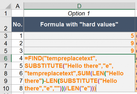
Finding the last occurrence of a string within a text is a little bit more complicated. You use SUBSTITUTE and LEN. The complete formula is like this:
=FIND(“tempreplacetext”;SUBSTITUTE(“Hello there”;”e”;”tempreplacetext”;SUM(LEN(“Hello there”)-LEN(SUBSTITUTE(“Hello there”;”e”;””)))/LEN(“e”)))
In order to understand the formula better, let’s start in the middle with the part SUM(LEN(“Hello there”)-LEN(SUBSTITUTE(“Hello there”;”e”;””)))/LEN(“e”)))
This part of the formula determines the number of “e” in “Hello there”. It replaces “e” in “Hello there” and the difference in the two versions (with and without e – “Hello there” and “Hllo thr”) is the number of “e”s.
The whole part SUBSTITUTE(“Hello there”;”e”;”tempreplacetext”;SUM(LEN(“Hello there”)-LEN(SUBSTITUTE(“Hello there”;”e”;””)))/LEN(“e”))) replaces the last “e” by “tempreplacetext”. Now you just put this into the FIND formula and get the position of “tempreplacetext”.
If you want to use this formula, replace all “e”s by your cell reference for the SEARCH TEXT and all “Hello there” by the cell reference to your WITHIN TEXT.
Replace text enclosed by brackets
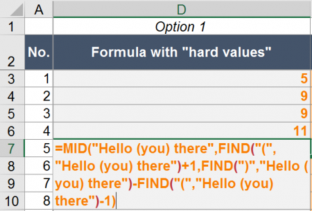
A last example for the FIND formula: You want to know what is written between two brackets. In such case, you can also use the FIND formulas in combination with the MID formula.
=MID(“Hello (you) there”,FIND(“(“,”Hello (you) there”)+1,FIND(“)”,”Hello (you) there”)-FIND(“(“,”Hello (you) there”)-1)
The MID formula returns some part of text from a (longer) text. It has three arguments:
- The initial, complete text.
- The starting character for the text you want to get.
- The length (in number of characters) of text you want to extract.
In our example above, the first FIND formula provides the character you want to start at. In our case that’s the first opening bracket (+1 because you want to start one character later). The second and third FIND formulas determine the length by
How to use the SEARCH formula
Like the FIND formula in Excel, SEARCH also returns the position of a text within another text.
Structure of the SEARCH formula

The SEARCH formula is very similar to the FIND formula. It has exactly the same arguments and works the same way.
Because of the, the structure is as follows:
- The SEARCH TERM is the text or character you search for.
- WITHIN TEXT contains the text you search in.
- The START NUMBER is optional and defines the number of character, after which Excel should start searching.
Yes, you are right – these arguments are exactly the same like in the FIND formula. But there is a major difference: SEARCH does not regard lower and upper case: It is not case sensitive. FIND on the other hand is case-sensitive and regards upper and lower cases.
Do you want to boost your productivity in Excel?
Get the Professor Excel ribbon!

Add more than 120 great features to Excel!
Examples for the SEARCH formula
The examples work exactly the same way like for the FIND formula. You only have to replace “FIND” by “SEARCH”. Because of that, we just show the summary below. If you want to know more, either scroll up to the “FIND”-examples or download the example workbook below.
| Example no. | Description | Formula |
| 6 | Return the position of “o” in “Hello there”. | =SEARCH(“o”,”Hello there”) |
| 7 | Return the position of “e” in “Hello there” after the third character. | =SEARCH(“e”,”Hello there”,3) |
| 8 | Return the position of the second occurrence of “e” in “Hello there”. | =SEARCH(“e”,”Hello there”,SEARCH(“e”,”Hello there”)+1) |
| 9 | Return the position of the last occurrence of “e” in “Hello there”. | =SEARCH(“tempreplacetext”,SUBSTITUTE(“Hello there”,”e”,”tempreplacetext”,SUM(LEN(“Hello there”)-LEN(SUBSTITUTE(“Hello there”,”e”,””)))/LEN(“e”))) |
| 10 | Return the text within brackets of “Hello (you) there”. | =MID(“Hello (you) there”,SEARCH(“(“,”Hello (you) there”)+1,SEARCH(“)”,”Hello (you) there”)-SEARCH(“(“,”Hello (you) there”)-1) |
Troubleshooting
The error message “#VALUE!” comes up most often for the FIND and SEARCH formulas. If you receive a “#VALUE!” error, please check the following possibilities.
- Make sure your SEARCH TERM can be found. If it can’t be found, you’ll receive the #VALUE! error.
- The last argument, the START NUMBER, is larger than the number of characters of in your WITHIN TEXT argument.
- You haven’t provided the last argument although you wrote the comma. For instance =SEARCH(“b”,”abc”,).
- Please check, if your SEARCH TERM and WITHIN TEXT have the same format. You can’t search for a letter or text in a number cell.
Difference between FIND and SEARCH
The first and major difference between FIND and SEARCH:
FIND is case-sensitive. SEARCH is not case-sensitive.
That means, FIND regards capital and small letter whereas SEARCH doesn’t.
How to remember which is which? I use the mnemonic:
- FIND finds exactly what you look for.
- Searching for something also searches for roughly what you look for.
I admit, it’s not the best mnemonic. Please let me know, if you have a better one!
There is also a second difference between FIND and SEARCH: You can use SEARCH with wildcard criteria within the SEARCH TERM.
- “?” stands for a single character. Example: =SEARCH(“?b”,”abc”)
- “*” matches any sequence of characters. =SEARCH(“*b”,”abc”)
- If you want to search exactly for ? or *, write a tilde in front of them. Example: =SEARCH(“~*”,”ab*c”)
Differences between FIND and FINDB as well as SEARCH and SEARCHB
Maybe you have noticed that there is also a slightly different version of the two formulas in Excel. If you add a “B” to the formulas, you can still use them the same way. So what is the difference?
FINDB and SEARCHB provide support for more complex languages. The definition by Microsoft is:
SEARCHB counts 2 bytes per character only when a DBCS language is set as the default language. Otherwise SEARCHB behaves the same as SEARCH, counting 1 byte per character.
According to Wikipedia DBCS stands mainly for the Asian languages Chinese, Japanese and Korean.
Please feel free to download all the examples shown above in this Excel file.
Click here and the download starts immediately.
 In an ideal world, you wouldn’t need to read this tutorial about some of the most important text formulas in Excel.
Unfortunately, we are not in ideal world…
If you work with Excel, you will need to know or learn how to use the LEFT, RIGHT, MID, LEN, FIND and SEARCH functions.
So… fortunately, you have found this tutorial which focuses on some of the most important text functions in Excel.
In this particular Excel tutorial, I explain step-by-step how you can use the LEFT, RIGHT, MID, LEN, FIND and SEARCH functions in Excel.
The following table of contents illustrates, more precisely, the topics we cover in this blog post. You can also use it to skip to the section that interests you the most.
This is a massive amount of content, so let’s begin by understanding…
Why You Should Learn How To Use The LEFT, RIGHT, MID, LEN, FIND And SEARCH Functions In Excel
You may rightly wonder why should you study this comprehensive 11,000+ word tutorial on Excel text formulas to learn how to use some of the most common Excel text functions.
There are several reasons why knowing how to use functions such as LEFT, RIGHT, MID, LEN, FIND and SEARCH is important. But instead of simply listing a bunch of reasons, allow me to ask you a question:
When working with Excel, there are times where you have to use data prepared by other people or companies. Based on your experience, how does this data look like? If you have never worked with data sets prepared by somebody else, please make a guess.
- Is it the data set clean, organized, and properly and consistently formatted?
- Or is it messy, disorganized, full of clutter and inconsistently formatted?
Let’s face it…
When you receive data prepared by other people or companies, you will need to clean up the data before you can proceed to work with it. In some cases, the data sets will be a complete mess.
And let’s not even talk about the situations where you have to work with several data sets, all prepared by different people who have completely different ideas about how the data should be organized (or disorganized).
When you use data from other sources, it’s usually not ready for analysis. Data scientists spend approximately 80% of their time in the process of gathering and cleaning up data before they can actually begin to analyze it.
The problem of messy data, however, is not exclusive to data analysts. There are many (other) examples. The main point to remember is that data quality is important. Therefore, knowing how to clean up data is essential.
What is the main take-away from the above?
You will need to clean up data. There is no question about it.
Sometimes you may also feel like this:
In order to avoid this type of situation, let’s ask a more relevant question: how will you clean up the data?
Will you do it manually? With the risks of missing errors or introducing new errors? Not to mention the amount of time cleaning up a large data set manually would take or how tedious the work would be…
Or will you automate the data clean-up process as much as possible to make it more streamlined and reliable?
If you are interested in learning how you can start automating the data clean-up process in Excel, keep reading. This Excel tutorial will make you significantly more efficient and productive, and reduce the risk of office violence.
I show you, step-by-step and using a very detailed example, how you can start using the LEFT, RIGHT, MID, LEN, FIND and SEARCH Excel functions now to improve your efficiency and productivity in Excel now.
You may be surprised by what you can do with Excel’s text functions. As explained by John Walkenbach in the Excel 2013 Bible:
(…) some of these formulas perform feats that you may not have thought possible.
Just as an example, quoting Excel Formulas and Functions for Dummies, mastering functions such as LEFT, RIGHT and MID “gives you the power to literally break text apart.”
Does this sound useful?
Then let’s start by understanding…
What Are Excel Text Functions
When you think about Excel, working with text is probably not the first thing that comes to your mind…
That is completely natural. After all, Excel is not a word processor… If you need a word processor, you can use Microsoft Word.
However, you may be surprised by Excel’s capabilities to handle and work with text. This is where Excel text functions come in…
Excel text functions are, as implied by their name, functions you can use to work with text or strings. For these purposes, as explained by John Walkenbach (one of the foremost authorities on Microsoft Excel) in the Excel 2013 Bible, text and string (and sometimes text string) are used interchangeably.
Despite the above, Walkenbach also explains how “many text functions are not limited to text” and, therefore, you can also use some of Excel’s text functions in cells that have numbers.
Excel has several text functions, which you can find by going to the Formulas tab of the Ribbon and clicking on “Text” or using the keyboard shortcut “Alt + M + T”.

What Is “Text”
I’ll ask you a question that may sound a little bit basic but, do you know what is text?
And I don’t mean regular text. I assume that, if you are reading this Excel tutorial, you know what is the usual definition of the word “text”.
The question is actually tricky because, in Excel, some things are slightly different from what you’d usually expect…
In Excel 2013 Formulas, John Walkenbach explains that whenever you type data, “Excel immediately goes to work and determines whether you are entering” one of the following:
- A formula.
- A number, which includes regular numbers, dates and times.
- Text, which is anything other than a formula or a number.
Believe it or not, it’s actually possible for Excel to treat a number as text. This is not that uncommon and, in some cases, can be quite annoying, such as when you are importing data into Excel.
It can also be quite dangerous as Excel does not always treat numbers that are formatted as text in the same way.
Let’s take a very simple example. The following Excel worksheet has two numbers in cells B1 and B2 (both numbers are 1). Cells B3 and B4 are reserved for the sum of these two numbers which you would expect to be 2 (as 1+1=2, right?).
Notice, however, that the numbers in cells B1 and B2 do not have the same alignment. The “1” in cell B1 is aligned to the left whereas the “1” in cell B2 is aligned to the right. This is because I have formatted cell B1 as text, something I may explain in future tutorials, and have not modified the alignment.

Now… let’s do some magic and see how, sometimes, 1 plus 1 doesn’t equal 2…
The screenshot below shows the result of calculating the sum of cells B1 and B2 using two different methods:
- In cell B3, the sum has been carried out by using the formula =B1+B2, as it appears in the parenthesis within cell A3.
- In cell B4, the sum has been calculated with the formula =SUM(B1:B2), as it appears inside the parenthesis in cell A4.
You can actually check out the formula bar to confirm that this is indeed the formula in the cell.

Don’t worry, you don’t have to go back to math lessons to review sums. Excel is indeed giving different treatments to cell B1 depending on which formula is used. In these cases, the SUM function treats cell B1 as a 0 and results in the sum of 1+1 not being equal to 2.
In this particular case, Excel indicates that there is a possible error (see the warning in the screenshot above) and the number in cell B1 is stored as text. According to John Walkenbach in Excel 2013 Formulas, this is usually the case (that Excel identifies the cell) if you have background error checking enabled.
However, as Walkenbach himself explains:
(…) be aware of Excel’s inconsistency in how it treats a number formatted as text.
Perhaps even better, be careful in general when using the text format and, when in doubt, use the general format.
Now that you know what exactly is “text” within Excel, allow me to introduce the example that I use in this tutorial on Excel text formulas:
My main business (as of the time of writing of this blog post) is real estate.
As you can imagine, our real estate company has to work a lot with addresses. Addresses for plots of land, buildings, houses and so on. You get the idea…
Sometimes we receive these addresses in big data sets prepared by somebody else and, as you may expect, their idea about how a database should be organized is different from mine.
Therefore, we constantly have to go through the process of cleaning up and fixing address data.
Address data is not only relevant for the real estate and construction industry. Databases where addresses can appear include, for example, the following:
- If you focus on sales, you may work constantly with lists of customers and may have to keep an organized list with their contact details.
- If you work at a company that operates several shops or branches, you may need to keep track of their individual addresses.
Therefore, the example I use to explain you how to use the LEFT, RIGHT, MID, LEN, FIND and SEARCH functions in Excel focuses on address data. More precisely, I take an address that I receive in a particular format and split the address into its different parts using Excel.
For these purposes, I have created 1,000 random addresses using a random address generator. They have all been pasted into a single column of an Excel worksheet.
This Excel Text Functions Tutorial is accompanied by Excel workbooks containing the data and formulas I use. You can get immediate free access to these example workbooks by subscribing to the Power Spreadsheets Newsletter.
The column with the full addresses in the initial Excel worksheet looks as follows:

Do you see any problems with the way this address list is organized?
Granted… it’s possible to get messier data. In this case all the addresses follow the same format, names are properly capitalized and, generally, the data looks relatively clean.
However, the data is organized in a way that may make it difficult to analyze using more advanced tools such as filters or PivotTables (topics I may explain in future tutorials). For example:
- Every single address is divided in two rows. The top row shows the street and number while the second row includes the city, state and zip code.

This is not very convenient if, for example, you want to have all the data of each customer in a single row. - Within a row, there are several details. As mentioned above, the first row includes both the street and number, and the second row lists the city, state and zip code.
Depending on the type of analysis you want to carry out with the data, it may be more useful if you are able to split these elements and show each item in a separate cell.

As a consequence of the above, I show you how to:
- Convert all addresses into a single row.
- Separate the elements of each address so that each item has its own individual cell.
More precisely, I show you step-by-step how to fill out the following table using Excel text formulas:

The steps in this example are chosen and structured considering that the main purpose is to show you, going slowly and step-by-step, how to use the LEFT, RIGHT, MID, LEN, FIND and SEARCH functions in Excel so you can apply and adapt these formulas by yourself later in different situations. There are other ways to achieve the same or similar results by using methods such as nesting functions within other functions, the text to columns command or, in some cases, slightly simpler formulas or tools that do not involve the LEFT, RIGHT, MID, LEN, FIND or SEARCH functions.
In certain cases, those other methods may be more appropriate and efficient to achieve your particular objectives. For example, instead of creating several columns (as I do in the process below), you can create a few nested functions that carry out all the required processes in less cells or use the text to columns command to parse the data.
However, nested functions, text to columns and similar tools deviate from the main purpose of this Excel tutorial: showing you how to use the LEFT, RIGHT, MID, LEN, FIND and SEARCH functions.
I agree, however, that there are different ways to perform the actions described in this Excel tutorial and I’m very interested in hear which other methods you would use to organize the addresses above. Please share your ideas and comments about how you would improve the process in the comments at the end of this guide.
I also mention and use some functions than are not explained in depth in this Excel tutorial, such as VALUE, ISNUMBER, IF and CONCATENATE. I may cover them in detail in future tutorials.
Are you ready?
Then let’s go on to the step-by-step explanation of how to use the LEFT, RIGHT, MID, LEN, FIND and SEARCH functions in Excel to fix these addresses.
Step #1: How To Use The LEFT Function In Excel To Determine Whether The First Character In A Cell Is A Number
One of the main problems with the original address list is that each address is spread over two rows of data.
Therefore, in the first few steps of this example, I show you how to solve this problem and get each address into a single row.
If you take a close look at the addresses, you’ll notice that the first row (where the street and number are) always begins with a numeric character while the second row (where the city, state and zip code appear) begins with an alphabetic character.

You can use this fact to distinguish between the rows of a single address. More precisely, you know that:
- If the first character in a cell is a number, this is the first row of the address.
- If the first character in a cell is not a number, this is the second row of the address.
So, the first thing you want Excel to do is determine whether the first character in a cell is a number or not.
I explain below, step-by-step, how you can do this:
1. Step #1: Use The LEFT Function To Grab The First Character Of The String.
The LEFT function allows you to find what the first characters in a text string are. You get to choose the number of characters that the LEFT function returns.
What is the syntax of the LEFT function?
The syntax of the LEFT function is “LEFT(text,num_chars)”, where:
- “text” is the text from which you want to extract the characters.
Here is where you tell Excel the location of the string from which you want to grab the characters or type the text within quotes “” (for example “This is the best Excel tutorial”).
- “num_chars” is the number of characters you want to extract.
The main requirement that num_chars must meet is that it can’t be a negative number. You can, however, specify a number of characters that is larger than those contained in the original string. In this case, the LEFT function simply returns the whole text.
You can also leave num_chars blank (omit it), in which case the LEFT function assumes it is 1 and return the first character of the text string.
So, how do you use the LEFT function to grab the first character of the addresses that are being cleaned up in the example?
For illustration purposes, I first create an additional column in the Excel worksheet that contains the addresses. This is column C and is titled “First Character”.

Now, let’s take a look at the syntax of the LEFT function, “LEFT(text,num_chars)”. In this case:
- “text” is the text located in column B.
- “num_chars” is 1.
It’s also possible to leave num_chars blank so that Excel assumes it is 1.
So the LEFT function is “LEFT(B#,1)”, where # is the number of the relevant row. For example, the formula for cell C3 is “=LEFT(B3,1)”:

And, in this case, the LEFT function returns 8, which is the first character of the address 857 King Street.

Now, you can copy and paste this formula across the 2,000 rows of data to get the LEFT function to return the main character of every single cell in the address list.

2. Step #2: Convert The Character You Have Extracted From The Text String Into A Number.
You are already aware of how, sometimes, Excel does not treat numbers as numbers. Remember how, above, I showed you that sometimes 1+1 is not equal to 2.
A similar thing may happen to the cells where the output of the LEFT function are.
For example, if you were to use the ISNUMBER function, which allows you to check if a value is a number and returns TRUE (if it is a number) or FALSE (otherwise) on cell C3 (which displays the number 8), the results are as follows:

Meaning that, according to Excel, the value in cell C3 is not a number.
To ensure that this does not cause any problems down the road, I convert the character that has been extracted from the text string to a number using the VALUE function. The VALUE function converts any text string that represents a number to an actual number for Excel purposes.
I may cover the VALUE function in detail in future Excel tutorials.
For the moment, is enough to know that the VALUE function has a single parameter which is the text that is converted to a number. In the example used in this Excel tutorial, this is the text located in column C.
Before applying the VALUE formula I add a new column to the Excel worksheet. This is column D titled “First Character Value”.

In this case, the formula for cell D3 is “=VALUE(C3)”.

And the result is the number 8:

You can copy and paste the formula in all the cells of column D to convert all of the text values that represent numbers in column C to actual numbers. Note that, in the cases where column C does not contain a number, but has a letter, the VALUE function returns “#VALUE”.
I fix this below.

3. Step #3: Check Whether The Character You Have Extracted Is A Number Or Not.
The ISNUMBER function allows you to check if a value is a number. If the value is indeed a number, ISNUMBER returns TRUE. If the value is not a number, ISNUMBER returns FALSE.
You can use the ISNUMBER function to check whether the first character you have extracted from the column of addresses is a number or not.
I may explain more about the ISNUMBER function in future Excel tutorials but, for the moment, is enough to know that ISNUMBER has a single parameter. This parameter is the particular value that you want Excel to test.
As usual, let’s add a new column to the Excel worksheet. This is column E and its title is “Is First Character a No.?”.

The formula for cell E3 is “=ISNUMBER(D3)”.

And the function returns TRUE, indicating that the value in cell D3 (and therefore the first character in the address) is a number.

You can copy and paste the formula in all the cells of column E to have Excel evaluate the values of the first character of the original text string. Notice how Excel, correctly, returns TRUE in the cases where the first character of the address cell is a number and FALSE when the first character is not a number.

If column E displays TRUE, that row is the first row of a particular address. This is because the first row of each address (where the street and number are) always begins with a number.
On the other hand, if column E shows FALSE, that particular row is the second row of an address (where the city, state and zip code appear) since those rows begin with alphabetic characters.
As a consequence of the above, you’re ready to move to the second step of cleaning up the address data…
Step #2: How To Use The IF Function In Excel To Place Each Full Address In A Single Row Of The Excel Worksheet
This particular step doesn’t focus on the functions and tools that are the main subject of this Excel tutorial. However, this step is important as it completes the process of putting each full address (which is originally divided in two rows) in a single row.
So let’s go ahead and do this…
1. Step #1: Use The IF Function To Get The First Part Of Each Address.
More precisely, you’re seeking to get the the street and number for each address.
The IF function allows you to check whether a condition is true or not and, based on the result, does one thing or another. Therefore, you can choose what the IF function should return if the condition is true or false.
For purposes of this tutorial, is important to understand its basic syntax: “IF(logical_test,value_if_true,value_if_false)”, where:
- “logical_test” is the condition you want to test.
- “value_if_true” is the value that the IF function returns if the condition you are testing is true.
- “value_if_false” is the value that the IF function returns if the condition you are testing is false.
How can you use this to get the first part of each address?
The first thing you probably want to look at is column E, since this tells you which rows have the first part of each address. Those rows are the ones where column E shows TRUE since, in those cases, the first character is a number (and all addresses begin with a number).
Therefore, you can use the IF function to:
- Test whether the value that appears in column E is equal to TRUE. This is the logical_test.
- If the condition you are testing is true, which is the case if that particular row contains the first part of an address, print that first part of the address (the street and number which appear in column B).
- If the condition you are testing is false, which happens if that row has the second part of an address, print nothing or leave the cell blank. This can be achieved by using quotes (“”).
How does this look in practice?
Let’s go back to the Excel worksheet…
First, I add a new column. This is column F and is titled “First Part of Address”.

The IF formula for cell F3 is “=IF(E3=TRUE,B3,””)”.

And, as expected, this returns the first part of the desired address.

You can copy and paste this formula in all the relevant cells. Check out how, as planned, column F displays the first part of the address or is blank.

2. Step #2: Use The IF Function To Get The Second Part Of The Address.
This time, you’ll be using the IF function to get the city, state and zip code for each address.
This step is basically the same as above with a couple of small tweaks. In this case, you can use the IF function as follows:
- Test whether column E shows TRUE. This is the same logical test used in the previous step.
- If the condition is true, print the second part of the address (the city, state and zip code that is displayed in column B).
Here is the main change in the syntax of the IF function when compared to the syntax used in the previous step. In the previous step you referred to the same row of the active cell whereas, now, you refer to one row below the active cell.
- If the condition you are testing is false, print nothing or leave the cell blank. This is exactly the same result as in the previous step.
Let’s start by adding an additional column to the Excel worksheet. This is column G and its title is “Second Part of Address”.

The IF formula for cell G3 is “=IF(E3=TRUE,B4,””)”. Notice that this is exactly the same formula used in the previous step except for the second parameter which has changed from cell B3 (same row as active cell) to cell B4 (one row below the active cell).

And, as planned, Excel returns the second part of the relevant address.

Just as in the previous step, you can copy and paste this formula to the 2,000 rows of column G. The results are substantially similar: Excel either returns the second part of the address or leaves the cell blank.

Step #3: How To Use Filters And Sorting To Delete Blank Rows In Excel Without Loosing Data
You may have noticed that, now that all addresses are in a single row, half of the cells in columns F and G are blank.

Those rows are no longer useful for purposes of fixing the addresses and, therefore, I show you how to delete them without loosing any data by using filters and sorting.
1. Step #1: Copy And Paste The Values Of All The Cells Located In Column G.
If you take a closer look at the IF formulas in column G, you’ll notice that they always make reference to a cell located in the row immediately below. As a consequence of this, if you delete all the rows that have blanks, you also delete the cells to which these formulas make reference to. For example, cell G3 makes reference to cell B4, as shown in the image below:

Deleting these references without any previous preparations leads to invalid cell reference errors appearing in column G. For example, in the case above:

You can avoid this type of error by copying all of column G and pasting its values.
To do this, proceed as follows. Below the step-by-step explanation there is an image illustrating how to perform all of these steps.
- Step #1: Click on the column letter header G.
- Step #2: In the Home tab of the Ribbon, click on “Copy”.
- Step #3: In the same Home tab, click on the drop-down menu button below “Paste”.
- Step #4: Once the drop-down menu expands, click on “Values”.
- Step #5: Excel pastes hard-coded values (not formulas) on all cells of column G.

Once you have done this, the cells in column G won’t have any formulas, just values. For example, in the case of cell G3:

2. Step #2: Using Filters, Sort Column F Or G From Highest To Lowest.
I may explain filters in more depth in future tutorials. For the moment is enough to know that you can use the sorting and filtering tools of Excel for purposes of rearranging your data, as shown below.
To do this, proceed as follows. I include an image below the step-by-step explanation showing how you can do this in Excel.
- Step #1: Select the headers of the table which, in this case, are located in row 2.
- Step #2: Go to the Data tab of the Ribbon and click on “Filter”.
- Step #3: Excel shows a drop-down arrow next to each header, showing that the filters are enabled but have not been applied.
- Step #4: Click on the drop-down arrow to the right of “First Part of Address” in cell F2 or “Second Part of Address” in cell G2.
- Step #5: When the full drop-down menu appears, click on “Sort Z to A”.
- Step #6: Excel sorts all the columns of the table based on the values of the column whose drop-down menu you have used for sorting purposes.

Why have I asked to sort the data like this?
If you scroll down to the middle of the table, you notice that the rows whose columns F and G appear empty are all in the lower half of the table.

This means that the 1,000 addresses are now all in the first 1,000 rows of the table and, therefore, you can proceed to eliminate rows 1,001 to 2,000.
3. Step #3: Delete Rows That Have Blank Cells In Columns F And G.
You can proceed as follows to delete all the rows that have blank cells in columns F and G. The image below the explanation illustrates all of these steps.
- Step #1: Select all of the rows to be deleted. You can do this by, for example, clicking on the row number header of the first row to be deleted, and then using the keyboard shortcut “Shift + Ctrl + down arrow”. This may take you all the way to the end of the Excel worksheet; don’t worry about it.
- Step #2: Right click on the row number headers.
- Step #3: A context menu appears.
- Step #4: Click on “Delete”.

Excel deletes all chosen rows. Now the table only has 1,000 rows, each corresponding to one of the 1,000 addresses.

4. Step #4: Disable The Filters.
You can disable the filters by clicking on “Filter” in the Data tab.
This step is optional; you can also carry on with the rest of this Excel tutorial while having the filters enabled.

Step #4:How To Use The RIGHT Function In Excel To Determine Whether The Last Character In A Cell Is A Space
Before I begin this section, I have to make the following clarification:
Usually you won’t use the method described in the following 3 steps (including steps #5 and #6) to deal with leading and trailing spaces in a text string. Instead of this, you’ll generally use the TRIM function.
However, I believe carrying out all activities with the functions we’re focusing on (LEFT, RIGHT, MID, LEN, FIND and SEARCH) gives you a better idea of the different things you can achieve with them.
Before we carry on, allow me to ask you the following question:
Based on the screenshot above, would you be able to say with certainty that there are no extra blank spaces at the end of an address?
For example, let’s focus on the first address: 999 River Street.

Would you be able to say with certainty that the letter t in Street is the last character and there are no blank spaces after it?
It is a tough question to answer, isn’t it?
And it is not a trivial question. As explained by John Walkenbach in Excel 2013 Formulas, extraneous spaces can cause problems in some cases, such as when using lookup formulas.
Fortunately, you can use the RIGHT function to take the guess work out of this.
The RIGHT function is, as you may expect, substantially similar to the LEFT function that I explained above. More precisely, the RIGHT function allows you to get the last (further to the right) characters in a text string. You decide, and tell Excel, how many characters it should return.
The syntax of the RIGHT function is, basically, the same as that of the LEFT function: “RIGHT(text,num_chars)”, where:
- “text” is the text string from which you want to get the characters.
This can be either the location of the text from which you want to extract the characters or a string within quotes (such as “I love Microsoft Excel”).
- “num_chars” is the number of characters you want the RIGHT function to give you back.
How many characters can you specify?As long as you don’t specify a negative number (which is not allowed), you should be fine.
Just note that, if you specify a number of characters that is larger than the length of the text string, the RIGHT function simply returns the whole string. Additionally, if you fail to specify a number, Excel assumes its 1 and return the last character of the string.
So let’s go ahead and use the RIGHT function to determine whether any of the two parts of the addresses has a blank space at the end.
As in previous occasions, I start by adding two columns to the right of the Excel worksheet. These are columns H and I, and are named “Last Character of First Part” and “Last Character of Second Part” respectively.

The formula for cell H3 is “=RIGHT(F3,1)”.

And the formula for cell I3 is “=RIGHT(G3,1)”.

You’ll notice that, according to the RIGHT function, the last character of the second part of the address is the number 2. This result was expected, as that is the last character of the zip code.
However, the cell with the last character of the first part shows nothing, meaning that it’s not the letter t but rather a space.

You can copy and paste these two formulas across all the rows of the table to see whether the other addresses have the same characteristic (the last character of their first part is a space).
As you can see in the results below, all of the cells in column H have no visible characters. They’re all spaces.

Sigh…
This means that one of the next steps in the process is to eliminate the extra space at the end of the first part of each address.
Could you do it using some of the functions that you have already learned in this tutorial?
Yes!
You can, for example, use the LEFT function to grab all the characters of the first part of the address except for the last one. In the next two steps, I show you one of the ways this can be done.
There are other ways to achieve this goal such as, for example, using the TRIM function. However, this is a topic that I’ll cover some other time.
Step #5: How To Use The LEN Function In Excel To Calculate The Number Of Characters In A Text String
Do you recall the syntax of the LEFT function?
That’s right, it’s “LEFT(text,num_chars)”.
If your purpose is to extract all the characters from the first part of the address except for the last one, the first question you may have is: how can you figure what is the character length of each of those strings of text?
That is a reasonable question. After all, the length of each address varies.
In this section, I introduce you a function that allows you to count the number of characters in a text string: the LEN function.
The LEN function counts and informs you what is the number of characters in a string. In other words, it tells you how long the text string is. The syntax of LEN is “LEN(text)”, where “text” is simply the string whose length you want to know.
Note that spaces, such as the ones that appear at the end of the first part of the addresses in the sample data set or between words, are also counted as characters.
As explained by Ken Bluttman in Excel Formulas and Functions for Dummies, LEN is usually used in conjunction with other functions such as LEFT, RIGHT or MID. In those cases, LEN is regularly used to set one of the parameters of the other function. I may explain in future tutorials how you can do this to create even more powerful Excel text formulas.
Before using the LEN function to calculate the number of characters in the first part of each address, I insert a new column in the Excel worksheet. This is column J and is named “Length of First Part of Address”.

Now you can proceed to measure the length of the first part of each address by using the LEN function. For example, the formula for cell J3 is “=LEN(F3)”

And LEN returns the number of characters in the first part of the address.

You can then, as usual, copy and paste the formula in all the relevant cells of column J to get Excel to calculate the length of the first part of each address.

Now that you have the length of the first part of each address, you can simply subtract one from each number to get the number of characters that you should extract from each string of text (using the LEFT function) to eliminate the extra space at the end.
For these purposes, I simply add a new column to the Excel worksheet (column J, titled “Proper Length of First Part of Address”) where I subtract 1 from the values obtained above.

After copying and pasting this formula in all the appropriate cells, the table looks roughly as follows:

Step #6: How To Use The LEFT Function To Get All The Characters In A Text String Except The Last One
By now, you have learned how to use the LEFT function in Excel and you know how many characters you need to extract from the first part of each address in order to exclude the last character.
So… do you know how to use the LEFT function to get all the characters, excluding the last one, in the first part of an address?
Let’s go through this process together…
First, I add a new column to the address table. This is column L and its title is “Proper First Part of Address”.

You already know the syntax of the LEFT function. For example, the formula for cell L3 is “=LEFT(F3,K3)”.

And Excel returns the first part of the address, excluding the last character. In this case, this means that the text string doesn’t have the extra space at the end.

You can then copy and paste it for all the rows in the table.

For organizational purposes, I add a new column to the table (column M with the title “Second Part of Address”), where I put the second part of each address. This way, the first and second part of the address are next to each other.

Step #7: How To Use The FIND And SEARCH Functions In Excel
Things are looking good, aren’t they?
Each address is in a single row and there are no extra spaces or extraneous characters.
However, the final objective of the example has not yet been achieved. I said at the beginning of this Excel tutorial that I’d show you how to fill out the following table using Excel text formulas:

In order to do this, I need to be able to extract each of these elements from the two parts of the addresses that currently appear in columns L and M.

As you probably imagine, it is possible to:
- Use functions such as LEFT and RIGHT to get the desired parts of each text string.
- Use LEN to calculate the number of characters to be extracted by the LEFT and RIGHT functions.
However, in this particular case, the situation is slightly more complicated than when using the LEFT and LEN functions to get the first part of the address without the last character.
The reason for this is that:
- In the previous steps, the length of the whole text string varied, but the number of characters to be excluded was fixed (it was always 1).
- Now, both the length of the text string and the length of the components to be included or excluded varies.
For example, street addresses (both the street and the number) and city names have different lengths.
State names have all the same length (2 characters) but, in order to be able to extract them using Excel text formulas (more precisely, using the MID function which I explain below), it’s necessary to know the position of the first character which, in turn, depends on the city name length.
Zip codes are more manageable. They are all 5 characters long and sit at the end of the string. Therefore, as you may have guessed, it is possible to extract them with the RIGHT function.
In any case, it’s necessary to find a way to measure the length of each of the different elements of the addresses.
How could you do this?
Allow me to introduce the FIND and SEARCH functions…
The FIND And SEARCH Functions In Excel
The FIND and SEARCH functions in Excel are substantially similar. Their purpose, as you may imagine from their names, is to find a particular piece of text within a text string.
What does this mean?
Let’s look at the rough idea graphically. Assume you are reading a book and you see the following text:

Now, imagine that you want to find the string of text “state Department”.
If you had the possibility to use the FIND or SEARCH functions of Excel, you could tell them something like: find the text string “state Department” within this page.
And Excel would tell you the location of the string “state Department”.

Now that you know the basic idea behind the FIND and SEARCH functions in Excel, let’s take a closer look at how they work in practice. From the explanation above, it is already clear that the main purpose of both FIND and SEARCH is to locate a particular text string within a longer text string.
How does Excel tell you the location of the text string you want to locate?
The FIND and SEARCH functions tell you where is the string you are searching for by returning a number that represents the starting position of that text string. Let’s take, for example, the first address in the sample data set: 999 River Street and assume you want to know the location of the word “River”.

In this case, Excel returns the number 5 because the starting position of the word “River” is the fifth character. The first 4 characters are 9, 9, 9 and space.
Let’s take a look now at the syntax of the FIND and SEARCH functions in Excel. The syntax of FIND is “FIND(find_text,within_text,start_num)” whereas the syntax of SEARCH is “SEARCH(find_text,within_text,start_num)”. In both cases:
- “find_text” is the string that you want to find. In the cases above, it is “state Department” or “River”.
- “within_text” is the text string where you want to search. In the cases above, it is the whole page or the Proper First Part of Address in the sample Excel worksheet.
- “start_num” is the character at which you want to start to search for the find_text within the within_text.
This argument is optional. If you leave it blank, Excel assumes it is 1 and begins the search on the first character of the within_text.
start_num is useful if, for example, you are only interested in the find_text that appears towards the end of a particular string of text.
For example, in the case of 999 River Street above, you may want to find the location of the second space (the one that separates the words “River” and “Street” but are not interested in knowing where the first space (that separates 999 from River) is. In such a case, you can set start_num to a number such as 6 (which, as explained above, is the starting position of the word “River”) and the FIND or SEARCH function return the number 10.
In fact, if you continue reading, you’ll notice that this is precisely one of the methods that I use below.
You probably have an additional question regarding the FIND and SEARCH functions…
Are FIND and SEARCH then the same function? Is there any difference between them?
Good question. There are, indeed, a couple of differences between FIND and SEARCH. The main ones are the following:
- FIND is case-sensitive whereas SEARCH is not.
For example, using the text from the cases above, FIND distinguishes between “state Department” and “state department” or between “River” and “river”. The SEARCH function doesn’t make such a distinction.
- SEARCH allows you to use the wildcard characters “?” (question mark) and “*” (asterisk) in find_text (the text you are searching for), whereas FIND does not.
What is the purpose of these wildcard characters?The question mark (?) character matches any single character. For example, in the case of 999 River Street above; if instead of searching for “River” you search for “R?ver”, Excel also searches for variants such as “Rover”.
The asterisk (*) character matches any sequence of characters. Continuing with the case of 999 River Street; if instead of searching for “River” you type in “Riv*”, Excel also looks out for different words that begin with “Riv” such as “Riviera”.
What should you do if you want to actually search for a question mark (?) or asterisk (*)?Type a tilde “~” before the question mark or asterisk. For example, if you want to search for “River?”, type “River~?” and if you want to search for “River*”, type “River~*”.
And… what should you do if you want to search for a tilde (~)?
Following with the logic of adding tildes before the special characters, in this case you need to type 2 tildes (~~).
Now you that you have a good understanding of both the FIND and SEARCH functions, let’s take a look at…
How To Apply The FIND Or SEARCH Functions To The Sample Data Set
The main purpose of introducing the FIND and SEARCH functions to you is to allow you to measure the length of each of the different elements of the addresses so that, in the following steps, you can get each individual item using the LEFT, RIGHT and MID functions.
Below, I explain to you how to do this.
Please note that I use and make reference to the SEARCH function. Theoretically, for this particular case, you can also use the FIND function since the searches do not use wildcard characters and there are no lowercase nor uppercase letters.
1. Step #1: Use The SEARCH Function To Locate Spaces And Commas.
Use SEARCH to find the location of:
- The first space in the first part of the address. This is the space that separates the street name from the number.
For example, in the case of the first address:

- The comma (,) in the second part of the address. This is the space that separates the city from the state.
For example, using the same case as above:
- The last space in the second part of the address. This is the space that separates the state from the zip code.
Continuing with the same example:


For clarity purposes, I add three new columns to the table. These columns are N, O and P. Their titles are “Location of First Space in First Part”, “Location of “,” in Second Part” and “Location of Last Space in Second Part”.

The formulas for the first two columns are relatively straightforward. After all, you know what is the text you are searching for (a space or a comma), what is the text you are searching in, and that you are searching from the beginning of the text.
Therefore, the formula for cell N3 is “=SEARCH(” “,L3)”.

Similarly, the formula in cell O3 is “=SEARCH(“,”,M3)”.

Both formulas return the expected results. For example, the location of the first space in the first part of the address is 4 (the first 3 characters are 9, 9 and 9) and the location of the comma in the second part is 7 (the first 6 characters are E, a, s, t, o and n).

The syntax of the third SEARCH formula, whose purpose is to find the last space in the second part of the address, is slightly more complicated.
If you take a close look at the second part of each address, you’ll notice that there are at least two spaces: one after the comma (,) that separates the city from the state, and one that separates the state from the zip code. There may be additional spaces if the city name is two words or longer.
You want the SEARCH function to return the location of the last space. This means that you need to specify a third parameter in the SEARCH function: the optional start_num argument which specifies the character at which you want to begin the search.
This is, however, not that simple. After all, city names have different lengths so you can’t just fix start_num.
To solve this small issue, let’s add a couple of intermediate steps.
First, I add an extra column in the Excel worksheet between the current columns O (Location of “,” in Second Part) and P (Location of Last Space in Second Part). This new column has the name “Beginning of State” and, as you see later, it comes in handy for other purposes in addition to finding the location of the last space in the second part of the address.

How do you know the number of the character at which the state begins?
You already know what is the number of the character at which the comma (,) that separates the city from the state is. This is the value that appears in column O (Location of “,” in Second Part).
Additionally, if you look closely at the format of the second part of all addresses, you’ll notice that after the comma there is a space (which is the first space in the second part). The state begins after that space.
As you have probably realized by now, the state begins 2 positions after the comma. Therefore, to find the number of the character at which the state begins you just need to add 2 to the value that appears in column O.
For example, the formula for cell P3 is “=O3+2”.

Once you know the position at which the state begins, you know that the next space is the last space in the second part of the address.
Therefore, you can use the position of the first character of the state as the starting point for the search of the last space in the text string (the start_num argument).
Considering the above, you can build a slightly more complex SEARCH function to find this last space. For example, the formula for cell Q3 is “=SEARCH(” “,M3,P3)”.

The newly added columns return the values that were expected so you can copy and paste the formulas in all the cells of columns N, O, P and Q to get all the relevant locations for each address.

2. Step #2: Determine Length Of Components Of First Part Of Address.
Use the data you have already calculated to determine the length of the different components in the first part of the address: namely the street name and number.
If you go back to column K of the Excel worksheet, you find the total length of the first part of the address after excluding the extra space at the end.

Additionally, in the step immediately prior to this one, you found the location of the space that separates the number and the street name. This value appears in column N of the Excel worksheet.

Using these two values, you can determine:
- The length of the number in the first part of the address.
You can find this by subtracting 1 from the location of the first space. This makes sense, since that space is just (1 character) after the end of the number
- The length of the street name.
You can calculate this by subtracting the location of the first space from the length of the whole text string. This makes sense, since that space is immediately (1 character) before the beginning of the street name.
Let’s do this…
For clarity purposes, I add (again) two new columns to the table in the Excel worksheet. These are columns R and S. Their titles are “Length of No.” and “Length of Street Name”.

And then I type in the relevant formulas. For example, the formula for cell R3 is “=N3-1”.

And the formula for cell S3 is “=K3-N3”.

As usual, you can simply copy and paste these formulas in the rest of the cells of those two columns to get the lengths of the street names and numbers for the rest of the addresses.

3. Step #3: Determine The Length Of The City Name.
You may wonder…
Wait! What happens with the length of the state and zip code? Don’t we need to calculate those too?
You can calculate the length of the states and zip codes for practicing purposes. However, this is not strictly necessary because they are always the same. More precisely:
- States are always 2 characters long.
- Zip codes are always 5 characters long.
So in reality, it’s only necessary to calculate the length of the city name.
Do you know how to do this calculation?
Hint: it’s very similar to the way we calculated the length of the number in the first part of the address.
Before you answer, let me add a new column to the Excel worksheet. This is column T and I name it “Length of City”.

You may have answered that the calculation of the length of any city name requires that you subtract 1 from the location of the comma in the second part of the address.
If this was your answer, you are correct! This makes sense due to the fact that the comma is immediately (1 character) after the end of the city.
Therefore, for example, the formula for cell T3 is “=O3-1”.

You can then proceed to copy and paste this formula in all the other rows of the table to have Excel calculate the length of each city name.

Step #8: How To Use The LEFT, RIGHT And MID Functions In Excel To Get The Individual Components Of Each Address
I am aware that this has been a long tutorial…
But you’re close to finishing.
This is the step, where you actually extract each of the components of each address to the table where each of them has its own column.

You can do most of this by using the LEFT and RIGHT functions which have been explained in this Excel tutorial. You, however, need to use the MID function to get the State data.
So, before going into the actual process of getting the data, let’s take a look at the MID function…
The MID Function In Excel
The MID function works similarly to the LEFT and RIGHT functions.
In particular, its purpose is substantially the same: to grab a certain amount of characters from a text string.
Why do you need the MID function if you already know how to use the LEFT and RIGHT functions?
You already know that you can use the LEFT function to get the first (furthest to the left) characters of a piece of text and the RIGHT function to extract the last (furthest to the right) characters of a string.
But… how can you get characters from the middle of a text string?
For example, in the case of the address database that has been used as an example in this Excel tutorial, how can you get the state data?

Theoretically, you can first apply the LEFT function to get the left portion of the address (up to and including the state) and, then, the RIGHT function to get the state. You can also do it the other way around: apply the RIGHT function followed by the LEFT function…
But using the MID function is simpler and doesn’t require you to go through multiple steps.
More precisely, the MID function returns a certain number of characters from the middle of a piece of text. It does this by starting at whichever position you specify in the formula and grabbing the amount of characters you determine.
The syntax of the MID function is “MID(text,start_num,num_chars)”, where:
- “text” is the string from which you want to get the characters.
- “start_num” is the position of the first character you want the MID function to get.
start_num can’t be a negative number.
Ideally, it should also be less than the length of the text from which the MID function is extracting the characters. The reason for this is that, if start_num is larger than the length of the text, the result returned by the formula is “” (empty).
Finally, as suggested by Ken Bluttman in Excel Formulas and Functions for Dummies, start_num should be a number larger than one. Why is this? Because, if you needed to begin to extract text from the beginning of the string, you could simply use the LEFT function.
- “num_chars” is the number of characters, or length, of the text string you want the MID function to return. This value can’t be a negative number.
If, for some reason, start_num (position of first character to be extracted) plus num_chars (number of characters to be grabbed) is more than the length of the text string from which the function is getting the characters, the MID function returns all the characters up to the end of the text. In this case, it has a similar effect to applying RIGHT (although the syntax is certainly different).
How To Use The LEFT, RIGHT And MID Functions To Get The Individual Components Of Each Address
By now you know how to use the LEFT, RIGHT and MID functions in Excel. You have also applied the LEFT and RIGHT functions to a couple of different situations.
So let’s go ahead and apply them to get the individual components of each address and fill the following table:

For ease of reference, I add the columns above to the left of the table in the original Excel worksheet. They are columns U through Z.

1. Step #1: Use The LEFT Function To Fill The “No.” Fields.
You know the text from which you want to extract the data (column L; Proper First Part of Address) and how many characters to get (column R; Length of No.).
You can build the relevant LEFT function with these two arguments. For example, the formula for cell V3 is “=LEFT(L3,R3)”.

Notice that the value returned by the LEFT function for the first address (999 River Street) is as expected (999).

2. Step #2: Use The RIGHT Function To Fill The Street Fields.
The text from which you want to get the data is the same as above (column L). In this case, the amount of characters to get appears in column S (Length of Street Name).
These two parameters are all you need to build the relevant RIGHT formula. For example, in the case of cell U3, the relevant formula is “=RIGHT(L3,S3)”.

Just as in the previous case, the text returned by the RIGHT function for the first address is the correct one (River Street).

3. Step #3: Fill The City By Using The LEFT Function.
The city is the first item in the second part of the address. Therefore, in this case, the string from which you want to extract the data is column M (Second Part of Address). The amount of characters to get is in column T (Length of City).
You are now ready to insert the LEFT formula. As an example, for cell W3, the formula is “=LEFT(M3,T3)”.

Once again, the formula returns the appropriate data (Easton).

4. Step #4: Use The MID Function To Get The Data For The State Fields.
Finally!
The chance for you to test the MID function.
Let’s recall the syntax of the MID function: “MID(text,start_num,num_chars)” and analyze each item separately:
- The string from which you want to extract the characters is the same as that from which you have gotten the city. Therefore, in the first argument, you make reference to column M.
- Maybe you remember that, when explaining how to use the FIND and SEARCH functions in Excel, I added column P (Beginning of State) and calculated what was the location of the first character of the state.
I also mentioned that this value would be useful later… and here it is the moment where you get to use it again.
You know that the position of the first character you want the MID function to get is in this column P. Therefore, you have the second argument for the formula.
- Finally, you know that the states are always 2 characters long.
Therefore, you are ready to insert the appropriate MID formula. For example, in cell X3, this is “=MID(M3,P3,2)”.

And Excel returns the correct values.

5. Step #5: Use The RIGHT Function To Obtain The Zip Code Data.
The zip code is the last item to extract.
As anticipated above, you are using the RIGHT function to extract the zip code.
The text from which you extract the data is the same as in the two cases above (column M). All zip codes are 5 characters long. This is all the data you need to create the relevant RIGHT function.
For example, for cell Y3, the formula is “=RIGHT(M3,5)”.

And you get the correct zip code as a result.

6. Step #6: Copy And Paste Formulas.
Copy and paste all the formulas in cells U through Y all the way down to the end of the table.

Congratulations!
You have completed all the steps of this Excel Text Formulas Tutorial that are related to how to use the LEFT, RIGHT, MID, LEN, FIND and SEARCH functions in Excel.
Additionally, your table is almost complete…
If you have the energy for a final step, I show you how to fill the last column of the table above…
Step #9: How To Use The CONCATENATE Function In Excel To Join All The Components Of An Address In A Single Cell
For the moment, you just need to know that the CONCATENATE function allows you to join different text strings into a single one. In this particular case, you use it to join the different components of each address, which you extracted in the step before, into a single cell.
The syntax of the CONCATENATE function is relatively simple: “CONCATENATE(text1,text2,…)”. In other words, the arguments of the CONCATENATE function are simply the text strings you want to join. As shown below, these arguments can also be strings (such as spaces or punctuation marks) surrounded by quotation marks (“”).
This is not too complicated, right?
So let’s go ahead and join all the components of an address in a single cell using the CONCATENATE function.
The form of the final joined addresses is “Street Name ###, City, State Zip Code”. This means that the first address should be River Street 999, Easton, PA 18042.
So how does the formula for this look like?
As you are probably aware, most of the text strings that are joined are in the last few columns (columns U through Y) of the table. These are the columns where the individual items of each address are stored.
However, you need to add spaces ( ) and commas (,). You can do this by using quotation marks (“”).
For example, the formula for cell Z3 is “=CONCATENATE(U3,” “,V3,”, “,W3,”, “,X3,” “,Y3)”.

And Excel returns the expected address.

Copy and paste this formula in all the rows of column Z and you are completely done.
Really!
The table is ready.

Conclusion
Once again…
Congratulations! You are ready to start using the LEFT, RIGHT, MID, LEN, FIND and SEARCH functions in Excel.
This Excel Text Functions Tutorial is accompanied by Excel workbooks containing the data and formulas I use above. You can get immediate free access to these example workbooks by subscribing to the Power Spreadsheets Newsletter.
I hope you agree that, despite their relative simplicity, these text functions are very powerful and useful. They are (usually) considered to be among the Excel functions everyone should know due to, among others, how much easier they make life when you are isolating pieces of text or cleaning up large data sets.
If you have completed this tutorial about Excel text formulas, you:
- Have a basic understanding of when you can use the LEFT, RIGHT, MID, LEN, FIND and SEARCH functions in Excel, and what these functions are capable of doing.
- Know the syntax of these formulas in order to be able to apply them in different situations.
You also have a basic understanding of some other functions and tools of Excel, such as the VALUE, ISNUMBER, IF and CONCATENATE functions, filters and sorting commands. I may cover these particular topics in more detail in future Excel tutorials but, using the information included in this guide, you can also start using them immediately.
There are other topics and methods you can learn for purposes of improving your efficiency and productivity when cleaning up data or carrying out similar activities with Excel that I have not covered in this guide. As I mentioned at the beginning of this tutorial about Excel text formulas, there are other methods that can be used to clean up the addresses that appear in the example that I used here.
Books Referenced In This Excel Tutorial
- Bluttman, Ken (2013). Excel Formulas and Functions For Dummies. Indianapolis, IN: John Wiley & Sons Inc.
- Walkenbach, John (2013). Excel 2013 Bible. Indianapolis, IN: John Wiley & Sons Inc.
- Walkenbach, John (2013). Excel 2013 Formulas. Hoboken, NJ: John Wiley & Sons Inc.