
Summary
This step-by-step article describes how to find data in a table (or range of cells) by using various built-in functions in Microsoft Excel. You can use different formulas to get the same result.
Create the Sample Worksheet
This article uses a sample worksheet to illustrate Excel built-in functions. Consider the example of referencing a name from column A and returning the age of that person from column C. To create this worksheet, enter the following data into a blank Excel worksheet.
You will type the value that you want to find into cell E2. You can type the formula in any blank cell in the same worksheet.
|
A |
B |
C |
D |
E |
||
|
1 |
Name |
Dept |
Age |
Find Value |
||
|
2 |
Henry |
501 |
28 |
Mary |
||
|
3 |
Stan |
201 |
19 |
|||
|
4 |
Mary |
101 |
22 |
|||
|
5 |
Larry |
301 |
29 |
Term Definitions
This article uses the following terms to describe the Excel built-in functions:
|
Term |
Definition |
Example |
|
Table Array |
The whole lookup table |
A2:C5 |
|
Lookup_Value |
The value to be found in the first column of Table_Array. |
E2 |
|
Lookup_Array |
The range of cells that contains possible lookup values. |
A2:A5 |
|
Col_Index_Num |
The column number in Table_Array the matching value should be returned for. |
3 (third column in Table_Array) |
|
Result_Array |
A range that contains only one row or column. It must be the same size as Lookup_Array or Lookup_Vector. |
C2:C5 |
|
Range_Lookup |
A logical value (TRUE or FALSE). If TRUE or omitted, an approximate match is returned. If FALSE, it will look for an exact match. |
FALSE |
|
Top_cell |
This is the reference from which you want to base the offset. Top_Cell must refer to a cell or range of adjacent cells. Otherwise, OFFSET returns the #VALUE! error value. |
|
|
Offset_Col |
This is the number of columns, to the left or right, that you want the upper-left cell of the result to refer to. For example, «5» as the Offset_Col argument specifies that the upper-left cell in the reference is five columns to the right of reference. Offset_Col can be positive (which means to the right of the starting reference) or negative (which means to the left of the starting reference). |
Functions
LOOKUP()
The LOOKUP function finds a value in a single row or column and matches it with a value in the same position in a different row or column.
The following is an example of LOOKUP formula syntax:
=LOOKUP(Lookup_Value,Lookup_Vector,Result_Vector)
The following formula finds Mary’s age in the sample worksheet:
=LOOKUP(E2,A2:A5,C2:C5)
The formula uses the value «Mary» in cell E2 and finds «Mary» in the lookup vector (column A). The formula then matches the value in the same row in the result vector (column C). Because «Mary» is in row 4, LOOKUP returns the value from row 4 in column C (22).
NOTE: The LOOKUP function requires that the table be sorted.
For more information about the LOOKUP function, click the following article number to view the article in the Microsoft Knowledge Base:
How to use the LOOKUP function in Excel
VLOOKUP()
The VLOOKUP or Vertical Lookup function is used when data is listed in columns. This function searches for a value in the left-most column and matches it with data in a specified column in the same row. You can use VLOOKUP to find data in a sorted or unsorted table. The following example uses a table with unsorted data.
The following is an example of VLOOKUP formula syntax:
=VLOOKUP(Lookup_Value,Table_Array,Col_Index_Num,Range_Lookup)
The following formula finds Mary’s age in the sample worksheet:
=VLOOKUP(E2,A2:C5,3,FALSE)
The formula uses the value «Mary» in cell E2 and finds «Mary» in the left-most column (column A). The formula then matches the value in the same row in Column_Index. This example uses «3» as the Column_Index (column C). Because «Mary» is in row 4, VLOOKUP returns the value from row 4 in column C (22).
For more information about the VLOOKUP function, click the following article number to view the article in the Microsoft Knowledge Base:
How to Use VLOOKUP or HLOOKUP to find an exact match
INDEX() and MATCH()
You can use the INDEX and MATCH functions together to get the same results as using LOOKUP or VLOOKUP.
The following is an example of the syntax that combines INDEX and MATCH to produce the same results as LOOKUP and VLOOKUP in the previous examples:
=INDEX(Table_Array,MATCH(Lookup_Value,Lookup_Array,0),Col_Index_Num)
The following formula finds Mary’s age in the sample worksheet:
=INDEX(A2:C5,MATCH(E2,A2:A5,0),3)
The formula uses the value «Mary» in cell E2 and finds «Mary» in column A. It then matches the value in the same row in column C. Because «Mary» is in row 4, the formula returns the value from row 4 in column C (22).
NOTE: If none of the cells in Lookup_Array match Lookup_Value («Mary»), this formula will return #N/A.
For more information about the INDEX function, click the following article number to view the article in the Microsoft Knowledge Base:
How to use the INDEX function to find data in a table
OFFSET() and MATCH()
You can use the OFFSET and MATCH functions together to produce the same results as the functions in the previous example.
The following is an example of syntax that combines OFFSET and MATCH to produce the same results as LOOKUP and VLOOKUP:
=OFFSET(top_cell,MATCH(Lookup_Value,Lookup_Array,0),Offset_Col)
This formula finds Mary’s age in the sample worksheet:
=OFFSET(A1,MATCH(E2,A2:A5,0),2)
The formula uses the value «Mary» in cell E2 and finds «Mary» in column A. The formula then matches the value in the same row but two columns to the right (column C). Because «Mary» is in column A, the formula returns the value in row 4 in column C (22).
For more information about the OFFSET function, click the following article number to view the article in the Microsoft Knowledge Base:
How to use the OFFSET function
Need more help?
На чтение 4 мин. Просмотров 478 Опубликовано 18.09.2019
Функция ROW в Excel возвращает номер строки ссылки. Функция COLUMN возвращает номер столбца. Примеры в этом уроке показывают, как использовать эти функции ROW и COLUMN.
Примечание . Инструкции в этой статье относятся к Excel 2019, Excel 2016, Excel 2013, Excel 2010, Excel 2019 для Mac, Excel 2016 для Mac, Excel для Mac 2011 и Excel Online.
Содержание
- Использование функции ROW и COLUMN
- Синтаксис и аргументы функций ROW и COLUMN
- Пример 1 – опустить ссылочный аргумент с помощью функции ROW
- Пример 2 – Использование ссылочного аргумента с функцией COLUMN
Использование функции ROW и COLUMN
Функция ROW используется для:
- Вернуть номер для строки данной ссылки на ячейку.
- Вернуть номер строки для ячейки, в которой находится функция на листе.
- Возвращает ряд чисел, идентифицирующих номера всех строк, где находится функция, при использовании в формуле массива.
Функция COLUMN используется для:
- Вернуть номер столбца для ячейки, в которой находится функция на листе.
- Вернуть номер для столбца данной ссылки на ячейку.
На листе Excel строки пронумерованы сверху вниз, причем строка 1 является первой строкой. Столбцы нумеруются слева направо, причем столбец A является первым столбцом.
Следовательно, функция ROW возвращает номер 1 для первой строки и 1 048 576 для последней строки листа.
Синтаксис и аргументы функций ROW и COLUMN

Синтаксис функции относится к макету функции и включает в себя имя функции, скобки и аргументы.
Синтаксис для функции ROW:
= СТРОКА (ссылка)
Синтаксис для функции COLUMN:
= COLUMN (ссылка)
Ссылка (необязательно). Ячейка или диапазон ячеек, для которых требуется вернуть номер строки или букву столбца.
Если ссылочный аргумент опущен, происходит следующее:
- Функция ROW возвращает номер строки ссылки на ячейку, в которой находится функция (см. Строку 2 в приведенных выше примерах).
- Функция COLUMN возвращает номер столбца ссылки на ячейку, в которой находится функция (см. Строку 3 в приведенных выше примерах).
Если для аргумента Reference введен диапазон ссылок на ячейки, функция возвращает номер строки или столбца первой ячейки в предоставленном диапазоне (см. Строки 6 и 7 в приведенных выше примерах).
Пример 1 – опустить ссылочный аргумент с помощью функции ROW

В первом примере (см. Строку 2 в приведенных выше примерах) пропускается аргумент Reference и возвращается номер строки в зависимости от расположения функции на листе.
Как и в большинстве функций Excel, функция может быть введена непосредственно в активную ячейку или введена с помощью диалогового окна функции.
Выполните следующие шаги, чтобы ввести функцию в активную ячейку:
- Выберите ячейку B2 , чтобы сделать ее активной.
- Введите формулу = ROW () в ячейку.
- Нажмите клавишу Enter на клавиатуре, чтобы завершить функцию.
Число 2 появляется в ячейке B2, так как функция находится во втором ряду рабочего листа.
Когда вы выбираете ячейку B2, полная функция = ROW () появляется на панели формул над рабочим листом.
Пример 2 – Использование ссылочного аргумента с функцией COLUMN

Во втором примере (см. Строку 3 в приведенных выше примерах) возвращается буква столбца ссылки на ячейку (F4), введенной в качестве аргумента ссылки для функции.
- Выберите ячейку B5 , чтобы сделать ее активной.
- Выберите вкладку Формулы .
- Выберите Поиск и справка , чтобы открыть раскрывающийся список функций.
- Выберите СТОЛБЦ в списке, чтобы открыть диалоговое окно «Аргументы функций».
- В диалоговом окне поместите курсор в строку Ссылка .
- Выберите ячейку F4 на листе, чтобы ввести ссылку на ячейку в диалоговом окне.
- Выберите ОК , чтобы завершить функцию и вернуться к рабочему листу.
Число 6 появляется в ячейке B5, поскольку ячейка F4 расположена в шестом столбце (столбец F) рабочего листа.
При выборе ячейки B5 полная функция = COLUMN (F4) появляется на панели формул над рабочим листом.
Поскольку в Excel Online нет вкладки «Формулы» на ленте, вы можете использовать следующий метод, который работает во всех версиях Excel.

- Выберите ячейку B5 , чтобы сделать ее активной.
- Нажмите кнопку Вставить функцию рядом с панелью формул.
- Выберите Поиск и справка в списке категорий.
- Выберите Столбец в списке и выберите ОК .
- Выберите ячейку F4 на листе, чтобы ввести ссылку на ячейку.
- Нажмите клавишу Ввод .
Число 6 появляется в ячейке B5, поскольку ячейка F4 расположена в шестом столбце (столбец F) рабочего листа.
При выборе ячейки B5 полная функция = COLUMN (F4) появляется на панели формул над рабочим листом.
Метод Find объекта Range для поиска ячейки по ее данным в VBA Excel. Синтаксис и компоненты. Знаки подстановки для поисковой фразы. Простые примеры.
Метод Find объекта Range предназначен для поиска ячейки и сведений о ней в заданном диапазоне по ее значению, формуле и примечанию. Чаще всего этот метод используется для поиска в таблице ячейки по слову, части слова или фразе, входящей в ее значение.
Синтаксис метода Range.Find
|
Expression.Find(What, After, LookIn, LookAt, SearchOrder, SearchDirection, MatchCase, MatchByte, SearchFormat) |
Expression – это переменная или выражение, возвращающее объект Range, в котором будет осуществляться поиск.
В скобках перечислены параметры метода, среди них только What является обязательным.
Метод Range.Find возвращает объект Range, представляющий из себя первую ячейку, в которой найдена поисковая фраза (параметр What). Если совпадение не найдено, возвращается значение Nothing.
Если необходимо найти следующие ячейки, содержащие поисковую фразу, используется метод Range.FindNext.
Параметры метода Range.Find
| Наименование | Описание |
|---|---|
| Обязательный параметр | |
| What | Данные для поиска, которые могут быть представлены строкой или другим типом данных Excel. Тип данных параметра — Variant. |
| Необязательные параметры | |
| After | Ячейка, после которой следует начать поиск. |
| LookIn | Уточняет область поиска. Список констант xlFindLookIn:
|
| LookAt | Поиск частичного или полного совпадения. Список констант xlLookAt:
|
| SearchOrder | Определяет способ поиска. Список констант xlSearchOrder:
|
| SearchDirection | Определяет направление поиска. Список констант xlSearchDirection:
|
| MatchCase | Определяет учет регистра:
|
| MatchByte | Условия поиска при использовании двухбайтовых кодировок:
|
| SearchFormat | Формат поиска – используется вместе со свойством Application.FindFormat. |
* Примечания имеют две константы с одним значением. Проверяется очень просто: MsgBox xlComments и MsgBox xlNotes.
В справке Microsoft тип данных всех параметров, кроме SearchDirection, указан как Variant.
Знаки подстановки для поисковой фразы
Условные знаки в шаблоне поисковой фразы:
- ? – знак вопроса обозначает любой отдельный символ;
- * – звездочка обозначает любое количество любых символов, в том числе ноль символов;
- ~ – тильда ставится перед ?, * и ~, чтобы они обозначали сами себя (например, чтобы тильда в шаблоне обозначала сама себя, записать ее нужно дважды: ~~).
Простые примеры
При использовании метода Range.Find в VBA Excel необходимо учитывать следующие нюансы:
- Так как этот метод возвращает объект Range (в виде одной ячейки), присвоить его можно только объектной переменной, объявленной как Variant, Object или Range, при помощи оператора Set.
- Если поисковая фраза в заданном диапазоне найдена не будет, метод Range.Find возвратит значение Nothing. Обращение к свойствам несуществующей ячейки будет генерировать ошибки. Поэтому, перед использованием результатов поиска, необходимо проверить объектную переменную на содержание в ней значения Nothing.
В примерах используются переменные:
- myPhrase – переменная для записи поисковой фразы;
- myCell – переменная, которой присваивается первая найденная ячейка, содержащая поисковую фразу, или значение Nothing, если поисковая фраза не найдена.
Пример 1
|
Sub primer1() Dim myPhrase As Variant, myCell As Range myPhrase = «стакан» Set myCell = Range(«A1:L30»).Find(myPhrase) If Not myCell Is Nothing Then MsgBox «Значение найденной ячейки: « & myCell MsgBox «Строка найденной ячейки: « & myCell.Row MsgBox «Столбец найденной ячейки: « & myCell.Column MsgBox «Адрес найденной ячейки: « & myCell.Address Else MsgBox «Искомая фраза не найдена» End If End Sub |
В этом примере мы присваиваем переменной myPhrase значение для поиска – "стакан". Затем проводим поиск этой фразы в диапазоне "A1:L30" с присвоением результата поиска переменной myCell. Далее проверяем переменную myCell, не содержит ли она значение Nothing, и выводим соответствующие сообщения.
Ознакомьтесь с работой кода VBA в случаях, когда в диапазоне "A1:L30" есть ячейка со строкой, содержащей подстроку "стакан", и когда такой ячейки нет.
Пример 2
Теперь посмотрим, как метод Range.Find отреагирует на поиск числа. В качестве диапазона поиска будем использовать первую строку активного листа Excel.
|
Sub primer2() Dim myPhrase As Variant, myCell As Range myPhrase = 526.15 Set myCell = Rows(1).Find(myPhrase) If Not myCell Is Nothing Then MsgBox «Значение найденной ячейки: « & myCell Else: MsgBox «Искомая фраза не найдена» End If End Sub |
Несмотря на то, что мы присвоили переменной числовое значение, метод Range.Find найдет ячейку со значением и 526,15, и 129526,15, и 526,15254. То есть, как и в предыдущем примере, поиск идет по подстроке.
Чтобы найти ячейку с точным соответствием значения поисковой фразе, используйте константу xlWhole параметра LookAt:
|
Set myCell = Rows(1).Find(myPhrase, , , xlWhole) |
Аналогично используются и другие необязательные параметры. Количество «лишних» запятых перед необязательным параметром должно соответствовать количеству пропущенных компонентов, предусмотренных синтаксисом метода Range.Find, кроме случаев указания необязательного параметра по имени, например: LookIn:=xlValues. Тогда используется одна запятая, независимо от того, сколько компонентов пропущено.
Пример 3
Допустим, у нас есть многострочная база данных в Excel. В первой колонке находятся даты. Нам необходимо создать отчет за какой-то период. Найти номер начальной строки для обработки можно с помощью следующего кода:
|
Sub primer3() Dim myPhrase As Variant, myCell As Range myPhrase = «01.02.2019» myPhrase = CDate(myPhrase) Set myCell = Range(«A:A»).Find(myPhrase) If Not myCell Is Nothing Then MsgBox «Номер начальной строки: « & myCell.Row Else: MsgBox «Даты « & myPhrase & » в таблице нет» End If End Sub |
Несмотря на то, что в ячейке дата отображается в виде текста, ее значение хранится в ячейке в виде числа. Поэтому текстовый формат необходимо перед поиском преобразовать в формат даты.
VLOOKUP is one of the most used functions in Excel. It looks for a value in a range and returns a corresponding value in a specified column number.
Now I came across a problem where I had to lookup entire row and return the values in all the columns from that row (instead of returning a single value).
So here is what I had to do. In the below dataset, I had Sales Rep names and the Sales they made in 4 quarters in 2012. I had a drop down with their names, and I wanted to extract the maximum sales for that Sales Rep in those four quarters.

I could come up with 2 different ways to do this – Using INDEX or VLOOKUP.
Lookup Entire Row / Column Using INDEX Formula
Here is the formula I created to do this using Index
=LARGE(INDEX($B$4:$F$13,MATCH(H3,$B$4:$B$13,0),0),1)
How it works:
Let first look at the INDEX function that is wrapped inside the LARGE function.
=INDEX($C$4:$F$13,MATCH(H3,$B$4:$B$13,0),0)
Let’s closely analyze the arguments of the INDEX function:
- Array – $B$4:$F$1
- Row Number – MATCH(H3,$B$4:$B$13,0)
- Column Number – 0
Notice that I have used column number as 0.
The trick here is that when you use column number as 0, it returns all the values in all the columns. So if I select John in the drop down, the index formula would return all the 4 sales values for John {91064,71690,67574,25427}.
Now I can use the Large function to extract the largest value
Pro Tip - Use Column/Row number as 0 in Index formula to return all the values in Columns/Rows.
Lookup Entire Row / Column Using VLOOKUP Formula
While Index formula is neat, clean and robust, VLOOKUP way is a bit complex. It also ends up making the function volatile. However, there is an amazing trick that I would share in this section. Here is the formula:
=LARGE(VLOOKUP(H3,B4:F13, ROW(INDIRECT("2:"&COUNTA($B$4:$F$4))), FALSE),1)
How it works
- ROW(INDIRECT(“2:”&COUNTA($B$4:$F$4))) – This formula returns an array {2;3;4;5}. Note that since it uses INDIRECT, this makes this formula volatile.
- VLOOKUP(H3,B4:F13,ROW(INDIRECT(“2:”&COUNTA($B$4:$F$4))),FALSE) – Here is the best part. When you put these together, it becomes VLOOKUP(H3,B4:F13,{2;3;4;5},FALSE). Now notice that instead of a single column number, I have given it an array of column numbers. And VLOOKUP obediently looks up values in all these columns and returns an array.
- Now just use LARGE function to extract the largest value.
Remember to use Control + Shift + Enter to use this formula.
Pro Tip - In VLOOKUP, instead of using a single column number, if you use an array of column numbers, it will return an array of lookup values.
You may also like the following Excel tutorials:
- VLOOKUP Vs. INDEX/MATCH
- How to make VLOOKUP Case Sensitive.
- How to Use VLOOKUP with Multiple Criteria.
- How to Sum a Column in Excel
- How to Return Cell Address Instead of Value in Excel
- How to Apply Formula to the Entire Column in Excel
We have the table in which the sales volumes of certain products are recorded in different months. It is necessary to find the data in the table, and the search criteria will be the headings of rows and columns. But the search must be performed separately by the range of the row or column. That is, only one of the criteria will be used. Therefore, you can`t apply the INDEX function here, but you need a special formula.
Finding values in the Excel table
To solve this problem, let us illustrate the example in the schematic table that corresponds to the conditions are described above.
The sheet with the table to search for values vertically and horizontally:
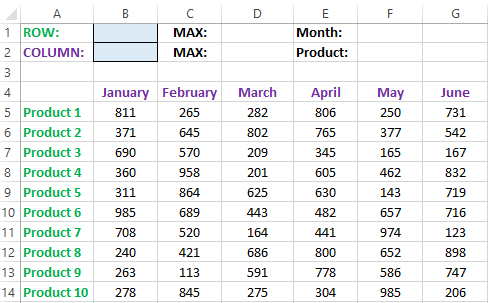
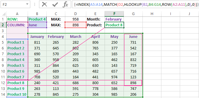
Above this table we can see the row with results. In the cell B1 we introduce the criterion for the search query, that is, the column header or the ROW name. And in the cell D1, to a search formula should return to the result of the calculation of the corresponding value. Then the second formula will work in the cell F1. She will already use the values of the cells B1 and D1 as the criteria for searching of the corresponding month.
Search of the value in the Excel ROW
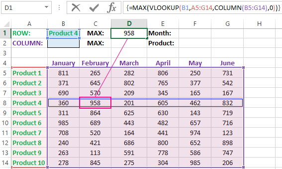
Now we are learning, in what maximum volume and in what month has been the maximum sale of the Product 4.
To search by columns:
- In the cell B1 you need to enter the value of the Product 4 — the name of the row, that will act as the criterion.
- In the cell D1 you need to enter the following:
- To confirm after entering the formula, you need to press the CTRL + SHIFT + Enter hotkey combination, because she must be executed in the array. If everything is done correctly, the curly braces will appear in the formula ROW.
- In the cell F1 you need to enter the second:
- For confirmation, to press the key combination CTRL + SHIFT + Enter again.
So we have found, in what month and what was the largest sale of the Product 4 for two quarters.
The principle of the formula for finding the value in the Excel ROW:
In the first argument of the VLOOKUP function (Vertical Look Up), indicates to the reference to the cell, where the search criterion is located. In the second argument indicates to the range of the cells for viewing during in the process of searching.
In the third argument of the VLOOKUP function should be indicated the number of the column from which you should to take the value against of the row named the Item 4. But since we do not previously know this number, we use the COLUMN function for creating the array of column numbers for the range B4:G15.
This allows the VLOOKUP function to collect the whole array of values. As a result, all relevant values are stored in memory for each column in the row Product 4 (namely: 360; 958; 201; 605; 462; 832). After that, the MAX function will only take the maximum number from this array and return it as the value for the cell D1, as the result of calculating.
As you can see, the construction of the formula is simple and concise. On its basis, it is possible in a similar way to find other indicators for a certain product. For example, the minimum or an average value of sales volume you need to find using for this purpose MIN or AVERAGE functions. Nothing hinders you from applying this skeleton of the formula to apply with more complex functions for implementation the most comfortable analysis of the sales report.
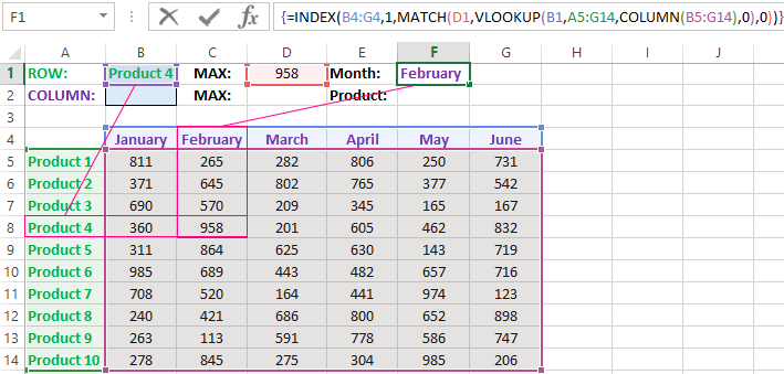
How can I get to the column headings from a single cell value?
For example, how effectively we displayed the month with the maximum sale, using of the second. It’s not difficult to notice that in the second formula we used the skeleton of the first formula without the MAX function. The main structure of the function is: VLOOKUP. We replaced the MAX on the MATCH, which in the first argument uses the value obtained by the previous formula. It acts as the criterion for searching for the month now.
And as a result, the MATCH function returns the column number 2, where the maximum value of the sales volume for the product is located for the product 4. After that, the INDEX function is included in the work. This function returns the value by the number of terms and column from the range specified in its arguments. Because the we have the number of column 2, and the row number in the range where the names of months are stored in any cases will be the value 1. Then we have the INDEX function to get the corresponding value from the range of B4:G4 — February (the second month).
Search the value in the Excel column
The second version of the task will be searching in the table with using the month name as the criterion. In such cases, we have to change the skeleton of our formula: the VLOOKUP function is replaced by the HLOOKUP (Horizontal Look Up) one, and the COLUMN function is replaced by the row one.
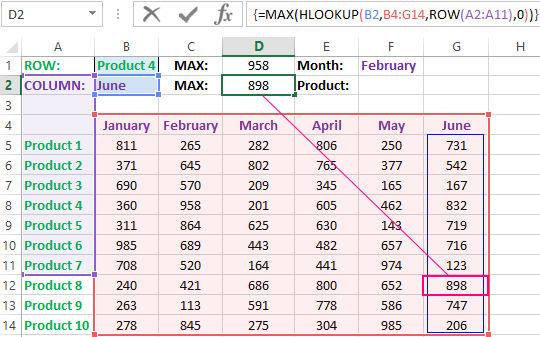
This will allow us to know what volume and what of the product the maximum sale was in a certain month.
To find what kind of the product had the maximum sales in a certain month, you should:
- In the cell B2 to enter the name of the month June — this value will be used as the search criterion.
- In the cell D2, you should to enter the formula:
- To confirm after entering the formula you need to press the combination of keys CTRL + SHIFT + Enter, as this formula will be executed in the array. And the curly braces will appear in the function ROW.
- In the cell F1, you need to enter the second:
- You need to click CTRL + SHIFT + Enter for confirmation again.
The principle of the formula for finding the value in the Excel column
In the first argument of the HLOOKUP function, we indicate to the reference by the cell with the criterion for the search. In the second argument specifies the reference to the table argument being scanned. The third argument is generated by the ROW function, what creates in the array of ROW numbers of 10 elements in memory. So there are 10 rows in the table section.
Further the HLOOKUP function, alternately using to each number of the row, creates the array of corresponding sales values from the table for the certain month (June). Further, the MAX function is left only to select the maximum value from this array.
Then just a little modifying to the first formula by using the INDEX and MATCH functions, we created the second function to display the names of the table rows according to the cell value. The names of the corresponding rows (products) we output in F2.
ATTENTION! When using the formula skeleton for other tasks, you need always to pay attention to the second and the third argument of the search HLOOKUP function. The number of covered rows in the range is specified in the argument, must match with the number of rows in the table. And also the numbering should begin with the second ROW!
Download example search values in the columns and rows
Read also: The searching of the value in a range Excel table in columns and rows
Indeed, the content of the range generally we don’t care — we just need the row counter. That is, you need to change the arguments to: ROW(B2:B11) or ROW(C2:C11) — this does not affect in the quality of the formula. The main thing is that — there are 10 rows in these ranges, as well as in the table. And the numbering starts from the second row!