
We have the table in which the sales volumes of certain products are recorded in different months. It is necessary to find the data in the table, and the search criteria will be the headings of rows and columns. But the search must be performed separately by the range of the row or column. That is, only one of the criteria will be used. Therefore, you can`t apply the INDEX function here, but you need a special formula.
Finding values in the Excel table
To solve this problem, let us illustrate the example in the schematic table that corresponds to the conditions are described above.
The sheet with the table to search for values vertically and horizontally:
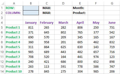
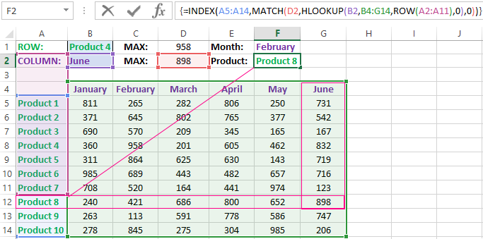
Above this table we can see the row with results. In the cell B1 we introduce the criterion for the search query, that is, the column header or the ROW name. And in the cell D1, to a search formula should return to the result of the calculation of the corresponding value. Then the second formula will work in the cell F1. She will already use the values of the cells B1 and D1 as the criteria for searching of the corresponding month.
Search of the value in the Excel ROW
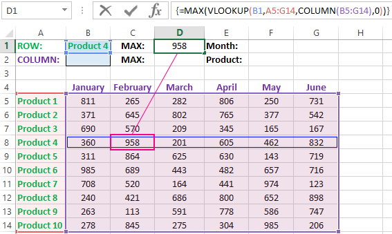
Now we are learning, in what maximum volume and in what month has been the maximum sale of the Product 4.
To search by columns:
- In the cell B1 you need to enter the value of the Product 4 — the name of the row, that will act as the criterion.
- In the cell D1 you need to enter the following:
- To confirm after entering the formula, you need to press the CTRL + SHIFT + Enter hotkey combination, because she must be executed in the array. If everything is done correctly, the curly braces will appear in the formula ROW.
- In the cell F1 you need to enter the second:
- For confirmation, to press the key combination CTRL + SHIFT + Enter again.
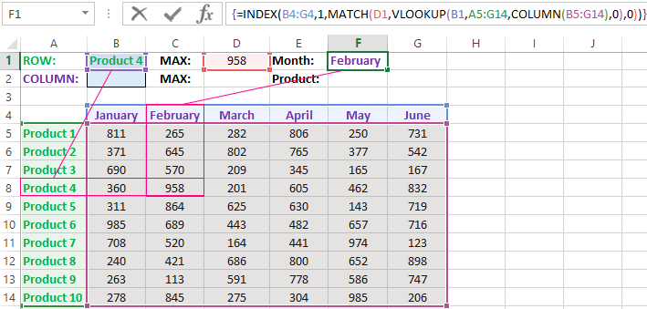
So we have found, in what month and what was the largest sale of the Product 4 for two quarters.
The principle of the formula for finding the value in the Excel ROW:
In the first argument of the VLOOKUP function (Vertical Look Up), indicates to the reference to the cell, where the search criterion is located. In the second argument indicates to the range of the cells for viewing during in the process of searching.
In the third argument of the VLOOKUP function should be indicated the number of the column from which you should to take the value against of the row named the Item 4. But since we do not previously know this number, we use the COLUMN function for creating the array of column numbers for the range B4:G15.
This allows the VLOOKUP function to collect the whole array of values. As a result, all relevant values are stored in memory for each column in the row Product 4 (namely: 360; 958; 201; 605; 462; 832). After that, the MAX function will only take the maximum number from this array and return it as the value for the cell D1, as the result of calculating.
As you can see, the construction of the formula is simple and concise. On its basis, it is possible in a similar way to find other indicators for a certain product. For example, the minimum or an average value of sales volume you need to find using for this purpose MIN or AVERAGE functions. Nothing hinders you from applying this skeleton of the formula to apply with more complex functions for implementation the most comfortable analysis of the sales report.
How can I get to the column headings from a single cell value?
For example, how effectively we displayed the month with the maximum sale, using of the second. It’s not difficult to notice that in the second formula we used the skeleton of the first formula without the MAX function. The main structure of the function is: VLOOKUP. We replaced the MAX on the MATCH, which in the first argument uses the value obtained by the previous formula. It acts as the criterion for searching for the month now.
And as a result, the MATCH function returns the column number 2, where the maximum value of the sales volume for the product is located for the product 4. After that, the INDEX function is included in the work. This function returns the value by the number of terms and column from the range specified in its arguments. Because the we have the number of column 2, and the row number in the range where the names of months are stored in any cases will be the value 1. Then we have the INDEX function to get the corresponding value from the range of B4:G4 — February (the second month).
Search the value in the Excel column
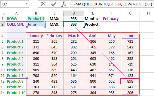
The second version of the task will be searching in the table with using the month name as the criterion. In such cases, we have to change the skeleton of our formula: the VLOOKUP function is replaced by the HLOOKUP (Horizontal Look Up) one, and the COLUMN function is replaced by the row one.
This will allow us to know what volume and what of the product the maximum sale was in a certain month.
To find what kind of the product had the maximum sales in a certain month, you should:
- In the cell B2 to enter the name of the month June — this value will be used as the search criterion.
- In the cell D2, you should to enter the formula:
- To confirm after entering the formula you need to press the combination of keys CTRL + SHIFT + Enter, as this formula will be executed in the array. And the curly braces will appear in the function ROW.
- In the cell F1, you need to enter the second:
- You need to click CTRL + SHIFT + Enter for confirmation again.
The principle of the formula for finding the value in the Excel column
In the first argument of the HLOOKUP function, we indicate to the reference by the cell with the criterion for the search. In the second argument specifies the reference to the table argument being scanned. The third argument is generated by the ROW function, what creates in the array of ROW numbers of 10 elements in memory. So there are 10 rows in the table section.
Further the HLOOKUP function, alternately using to each number of the row, creates the array of corresponding sales values from the table for the certain month (June). Further, the MAX function is left only to select the maximum value from this array.
Then just a little modifying to the first formula by using the INDEX and MATCH functions, we created the second function to display the names of the table rows according to the cell value. The names of the corresponding rows (products) we output in F2.
ATTENTION! When using the formula skeleton for other tasks, you need always to pay attention to the second and the third argument of the search HLOOKUP function. The number of covered rows in the range is specified in the argument, must match with the number of rows in the table. And also the numbering should begin with the second ROW!
Download example search values in the columns and rows
Read also: The searching of the value in a range Excel table in columns and rows
Indeed, the content of the range generally we don’t care — we just need the row counter. That is, you need to change the arguments to: ROW(B2:B11) or ROW(C2:C11) — this does not affect in the quality of the formula. The main thing is that — there are 10 rows in these ranges, as well as in the table. And the numbering starts from the second row!
I would not use MATCH to get the row number since you have multiple criteria. I would still use INDEX however to get the value of the row in E once the proper row number was discovered.
So instead of MATCH I would use an array formula using an IF statement that contained multiple criteria. Now note that array formulas need to be entered using ctrl + shift + enter. The IF statement would look like this:
=IF((A1>=C:C)*(A1<=D:D),ROW(A:A),"")
Note: I did not use the AND formula here because that cannot take in arrays. But since booleans are just 1’s or 0’s in Excel, multiplying the criteria works just fine.
This now gives us an array containing only blanks and valid row numbers. Such that if rows 5 and 7 were both valid the array would look like:
{"","","","",5,"",7,"",...}
Now if we encapsulate that IF statement with a SMALL we can get whatever valid row we want. In this case since we just want the first valid row we can use:
=SMALL(IF((A1>=C:C)*(A1<=D:D),ROW(A:A),""),1)
Which if the first valid row is 5 then that will return 5. Incrementing the K value of the SMALL formula will allow you to grab the 2nd, 3rd, etc valid row.
Now of course since we have the row number a simple INDEX will get us the value in column E:
=INDEX(E:E,SMALL(IF((A1>=C:C)*(A1<=D:D),ROW(A:A),""),1))
-
Excel Howtos
Extracting numbers from text in excel [Case study]
-
Last updated on June 19, 2012

Chandoo
Often we deal with data where numbers are buried inside text and we need to extract them. Today morning I had such task. As you know, we recently ran a survey asking how much salary you make. We had 1800 responses to it so far. I took the data to Excel to analyze it. And surprise! the numbers are a mess. Here is a sample of the data.

Now, how do I extract the salary amounts from this without typing the values?
My first thought is to write a user defined function to extract the number from text. But I usually shy away from VBA. So I wanted to see if there is a formula based approach to extract the number from text.
Using formulas to extract number from text

To extract number from a text, we need to know 2 things:
- Starting position of the number in text
- Length of the number
For example, in text US $ 31330.00 the number starts at 6th letter and has a length of 8.
So, if we can write formulas to get 1 & 2, then we can combine them in MID formula to extract the number from text!
Finding the starting position of number in text
To find the starting position, we need to find the first character which is a number (0 to 9). In other words, if we can find the positions of 0 to 9 inside the given text, then the minimum of all such positions would be starting position.
Sounds complicated?!? Well, in that case look at the formula and then you will understand why this works.
Assuming the text is in A1 and the range lstNumbers contains 0 to 9, below formula finds starting position
{=MIN(IFERROR(FIND(lstNumbers,A1),””))}
You need to array enter it (CTRL+SHIFT+Enter)
How this formula works?
FIND(lstNumbers, A1) portion: This part finds where each of the numbers 0 to 9 occur in the text in A1. If a match is found, the position is returned. Else we get an error. For US $ 31330.00 the values would be,
{10;7;#VALUE!;6;#VALUE!;#VALUE!;#VALUE!;#VALUE!;#VALUE!;#VALUE!}
Meaning, 0 occurs at 10th position, 1 occurs at 7th position, 3 occurs at 6th position and everything else (2,4,5,6,7,8,9) do not occur in the number.
IFERROR(…,””) portion: Then, we replace errors with empty spaces so that MIN could work its magic.
At this stage, the result would be, {10;7;””;6;””;””;””;””;””;””}
Related: IFERROR Formula – syntax & examples
{=MIN(…)} portion: This would find the minimum of {10;7;””;6;””;””;””;””;””;””} which is 6. The starting position of number inside text.
Because we are finding multiple items, we need to array enter the formula to get correct result.
Finding the length of number
Once we find starting point, next we need to know the length of the number. There are many ways to do this. Depending on the variety in your input data, you can choose a technique that works best.
Approach 1 – counting number of digits in text
My first approach is to count number of digits in the text and use it as length. For this, we can break the text in to individual characters and then see if each of them is a number or not.
Assuming the text is in A1, the number of digits in it are,
=SUMPRODUCT(- -ISNUMBER(MID(A1,ROW($A$1:$A$200),1)+0))
MID(A1,ROW($A$1:$A$200),1) + 0 portion: This breaks the text in A1 in to individual characters (assumes the max length is 200) and then adds 0 to them.
At this stage, you have 200 values some of them numbers, others errors.
ISNUMBER(…) portion: This checks all the 200 values for numbers. After this, we will have 200 true or false values.
— ISNUMBER (…) portion: This converts the true, false values to 0s and 1s. (by double negating Excel will convert boolean values to number equivalents).
SUMPRODUCT(…) portion: This finally sums up all 1s thus giving us the number of digits in the text.
Does it work?
While this approach works well for some numbers, it fails in other cases. For example, a text like US $ 31330.00 has number portion with 8 characters (31330.00) where as our formula would say the length is 7 (because decimal point . is not a number and hence ISNUMBER() would give false for that).
So I had to move on to next approach.
Approach 2 – counting number of digits, commas & decimal points in text
The next approach is to count not only numbers, but also commas & decimal points in the text. For this, first I placed all the digits (0 to 9) and comma & decimal point in a range called as lstDigits.
Below formula counts how many of lstDigits are in text in A1.
=SUMPRODUCT(COUNTIF(lstDigits,MID(A1,ROW($A$1:$A$200),1)))
COUNTIF(lstDigits, MID(…)) portion: This checks how many times each of the 200 characters appear in lstDigits.
This would be an array of counts. For example {0;0;0;0;0;1;1;1;1;1;1;1;1;…} for US $ 31330.00, indicating that first 5 are not in lstDigits and then we have 8 in lstDigits.
SUMPRODUCT(…) portion: just sums all the numbers, hence we get length as 8.
Related: SUMPRODUCT Formula – examples & explanation

Extracting numbers from text
Once we have starting position of number & its length, we can combine them in a MID formula to extract the number. Here is the result for our sample data set.
As you can see, this method works well, but fails in some cases like,
- European number formats (, for decimal point and . for thousands)
- Text with multiple numbers
Fortunately, in my data set, we had only a few incidents like these. So I have decided to manually adjust them than work out even more complicated formula.
Using Macros to extract numbers from text
As you can guess, we can use a simple macro (or UDF) to extract numbers from a given text. We will learn how to do this next week.
Download Example Workbook
Click here to download example workbook with all these formulas. Examine the formulas to understand how you can extract numbers from text in Excel.
Often I deal with data like this. I use a mix of techniques. Apart from the one mentioned above I also use,
- getNumber() UDF to extract numbers from text (more on this next week)
- Use SUBSTITUTE to clear formatting (replace dots with empty spaces and commas with dots to convert from European format to standard format)
- Use VALUE to extract the number (works when number is shown as text)
- Use +0 to force convert numbers from text (works when number is shown as text)
What about you? How do you extract numbers from text? What are your favorite techniques? Please share using comments.
Tips on cleaning data using Excel
If you use Excel to clean data, go thru these articles to learn some powerful techniques.
- Clean up dates & convert text to dates
- Remove Duplicates using Excel using formulas or using Excel features
- Extract phone numbers from data
- Quickly fill blank cells with data
Share this tip with your colleagues

Get FREE Excel + Power BI Tips
Simple, fun and useful emails, once per week.
Learn & be awesome.
-
65 Comments -
Ask a question or say something… -
Tagged under
advanced excel, array formulas, cleanup data, downloads, Excel Howtos, find, iferror, Learn Excel, Microsoft Excel Formulas, MIN(), sumproduct
-
Category:
Excel Howtos

Welcome to Chandoo.org
Thank you so much for visiting. My aim is to make you awesome in Excel & Power BI. I do this by sharing videos, tips, examples and downloads on this website. There are more than 1,000 pages with all things Excel, Power BI, Dashboards & VBA here. Go ahead and spend few minutes to be AWESOME.
Read my story • FREE Excel tips book


Excel School made me great at work.
5/5

From simple to complex, there is a formula for every occasion. Check out the list now.

Calendars, invoices, trackers and much more. All free, fun and fantastic.

Power Query, Data model, DAX, Filters, Slicers, Conditional formats and beautiful charts. It’s all here.

Still on fence about Power BI? In this getting started guide, learn what is Power BI, how to get it and how to create your first report from scratch.

- Excel for beginners
- Advanced Excel Skills
- Excel Dashboards
- Complete guide to Pivot Tables
- Top 10 Excel Formulas
- Excel Shortcuts
- #Awesome Budget vs. Actual Chart
- 40+ VBA Examples
Related Tips
65 Responses to “Extracting numbers from text in excel [Case study]”
-
 Gregor Erbach says:
 I have learned one important lesson in my career: don’t use Excel as a word processor!
Excel is very ill-suited to handling tasks like pattern matching in text (regular expressions).
For example, one could use a Perl script (from the CMD command line) to extract numbers from the text, something like
perl -n -e «m/([d,.]*)/; print «$1n» IN > OUT
The point I am trying to make is, if text processing is a substantial part of your tasks, it is worth the effort learning a tool that is more suited to the task.-
I agree with what your saying about suitability of tools to task,
but seriously perl -n -e “m/([d,.]*)/; print “$1n” IN > OUT
Doesn’t just roll off your tongue
and very few PC’s would even have Perl installed
-
Interesting point. I would have used VBA or some variation of that to clean data. But as Hui says Perl is not something many (including me) have on our computers. Plus I suck at regular expressions. I have tried long and hard to learn them, but I guess my mind is not wired to understand how they work 🙁
-
Jim says:
The VBA engine for regular expressions works fine in Excel and Access. I agree if you are doing a substantial amount of text cleaning then doing so exclusively in Excel is probably not the best course, but using regular expressions in Perl or any other flavor doesn’t really provide any advantage over using regex in Excel. At the end of the day, regex is regex (with the exception of minor syntactic differences).
Chandoo, a lot of people are intimidated by regex just like people are intimidated by formulas or macros. Once you learn a handful of rules and concepts, you can really do some damage with regex, and not just for data cleaning. You can validate input, parse, transform (e.g. firstname lastname —> lastname, firstname), etc. Once you pick it up you’ll see many opportunities where it’s useful and sometimes superior to another approach (and sometimes not). My brain is not wired to understand multiple nested formulas or complicated array formulas so I guess regex is just easier to me. I would add that the regular expression approach not only cleans this data, but is flexible enough to account for other variations…try it on the other records you have and see how well it performs. Either way, it’s great to know there are multiple approaches to solving the problem!
-
-
Bhavani Seetal Lal says:
How to sign inn into chandoo.org???
-
Vijay Kumar says:
Dear Chandoo…
Awesome, you are such a genius, how can you think like «what the excel will think»? Such ideas implementation…Very great . But lastly, i just wanted to know that in your formula =SUMPRODUCT(COUNTIF(lstDigits,MID(B4,ROW($A$1:$A$200),1))), why we can’t use 1 on behalf of ROW($A$1:$A$200), obviously if we will input this formula somewhere in excel, it results 1. So what is the logic to use row function instead of simple 1.
Please explain, i am eager to learn the logic of inputting or building a formulas. Can you suggest me the source like web url or books to build better formulas in our excel work
-
Luke M says:
Within SUMPRODUCT, that bit of formula is actually producing an array of numbers from 1 to 200, eg
{1,2,3,4,…200}
To see this in the formula, highlight that portion within the SUMPRODUCT and hit F9.
-
-
In the first example above, I would store lstNumbers as a Named Formula:
lstNumbers ={0;1;2;3;4;5;6;7;8;9}
-
I do not know why you would not want to use a UDF — Here is the code for one I wrote that extracts Numbers, Letters, Commas and spaces to clean up data — amend as you wish for ANY ASCII characters
Function NumbersAndLettersOnly(instring) As String
Dim StringLength As Integer ‘to hold string length
Dim i As Integer ‘counter for loop
Dim AsciiVal ‘to hold working character
Dim WorkingString As String ‘to build output string
instring = Trim(instring) ‘Drop leading & trailing spaces
StringLength = Len(instring) ‘Count number of characters in string
For i = 1 To StringLength ‘Loop thru each character in the string
AsciiVal = Asc(Mid(instring, i, 1))
If AsciiVal >= 48 And AsciiVal <= 57 Then ‘Numbers 0-9
WorkingString = WorkingString & Chr(AsciiVal)
ElseIf AsciiVal >= 65 And AsciiVal <= 90 Then ‘A-Z
WorkingString = WorkingString & Chr(AsciiVal)
ElseIf AsciiVal >= 97 And AsciiVal <= 122 Then ‘a-z
WorkingString = WorkingString & Chr(AsciiVal)
ElseIf AsciiVal = 46 Then ‘.
WorkingString = WorkingString & Chr(AsciiVal)
ElseIf AsciiVal = 32 Then ‘{space}
WorkingString = WorkingString & Chr(AsciiVal)
End If
Next i
NumbersAndLettersOnly = WorkingString ‘Return output to function
End Function-
@Cliff,
In case you might be interested, here is a shorter UDF which does the same thing as the one you posted…
[code]
Function AlphaNumerics(ByVal InString) As String
Dim X As Integer
For X = 1 To Len(InString)
If Mid(InString, X, 1) Like «[!A-Za-z0-9. ]» Then Mid(InString, X, 1) = Chr$(1)
Next
AlphaNumerics = Replace(InString, Chr$(1), «»)
End Function
[/code]-
Kevin says:
I used this one, because it was the smallest but most readable (to me).
The quotes didn’t translate correctly into VBA when I cut and pasted, so I just deleted them and typed them in again. Also, this function does the opposite: it finds the search characters in the 1st set of quotes, and then substitutes a null character. In my case, I wanted the opposite, so I just added a NOT in front of Mid. Thanks Rick. 🙂
-
-
-
Hi Purna,
I had a similar request earlier this week. Here’s the ‘quick & dirty’ solution I used. Keep in mind that, if there are a lot of different characters and text you need to remove from your text, this can get a little cumbersome. But for removing a few different text strings and characters from the same cell, this is pretty simple to understand.Using your example, to remove the space character , INR, and Rs, I would use this formula…
=SUBSTITUTE(SUBSTITUTE(SUBSTITUTE(B4,» «,»»),»INR»,»»),»Rs»,»»)
You start with =SUBSTITUTE(B4,» «,»») and then wrap it in another SUBSTITUTE for each text string you want to remove.
-
Elias says:
One more option that works withh all Excel versions.
=1*
MID(A1,
MIN(FIND({0,1,2,3,4,5,6,7,8,9},A1&»0123456789″)),
FIND(» «,A1&» «,MIN(FIND({0,1,2,3,4,5,6,7,8,9},A1&»0123456789»)))
)Confirm with Cntrl+Shift+Enter
Regards
-
Elias says:
Other more with different approach.
=1*
MID(A1,
MATCH(1,1*ISNUMBER(1*MID(A1,ROW($1:$255),1)),0),
MATCH(10,1*MID(A1,ROW($1:$255),1))
)Ctrl+Shift+Enter
Regards
-
Isaac says:
You just saved me from giving up haha. I tried many formulas that didn’t work, this one did it!!! Thank You very much
-
@Isaac
Never give up
The Chandoo.org Forums are a great source of asking «How do I …» questions and getting a result real quick
http://chandoo.org/forums/
-
-
-
Okay, one more method. The following was posted some time ago by Lars-Åke Aspelin in some forum or newsgroup…
=MID(SUMPRODUCT(—MID(«01″&A1,SMALL((ROW($1:$300)-1)*ISNUMBER(-MID(«01″&A1,ROW($1:$300),1)),ROW($1:$300))+1,1),10^(300-ROW($1:$300))),2,300)
This is an array formula and has to be confirmed with CTRL+SHIFT+ENTER rather than just ENTER.
It has the following (known) limitations:
— The input string in cell A1 must be shorter than 300 characters
— There must be at most 14 digits in the input string.
(Following digits will be shown as zeroes.)
Maybe of no practical use, but it will also handle the following two cases correctly:
— a «0» as the first digit in the input will be shown correctly in the output
— an input without any digits at all will give the empty string as output (rather than 0). -
Jim says:
I would probably use regular expressions in this case. The functions are:
************************************************
Function RegExReplace(ReplaceIn, _
ReplaceWhat As String, ReplaceWith As String, Optional IgnoreCase As Boolean = False)
Dim RE As Object
Set RE = CreateObject(«vbscript.regexp»)
RE.IgnoreCase = IgnoreCase
RE.Pattern = ReplaceWhat
RE.Global = True
RegExReplace = RE.Replace(ReplaceIn, ReplaceWith)
End FunctionFunction RegExFind(FindIn, FindWhat As String, _
Optional IgnoreCase As Boolean = False)
Dim i As Long
Dim matchCount As Integer
Dim RE As Object, allMatches As Object, aMatch As Object
Set RE = CreateObject(«vbscript.regexp»)
RE.Pattern = FindWhat
RE.IgnoreCase = IgnoreCase
RE.Global = True
Set allMatches = RE.Execute(FindIn)
matchCount = allMatches.Count
If matchCount >= 1 Then
ReDim rslt(0 To allMatches.Count — 1)
For i = 0 To allMatches.Count — 1
rslt(i) = allMatches(i).Value
Next i
RegExFind = rslt
Else
RegExFind = «»
End If
End Function************************************************
and the usage is:
=RegExFind(B4,»d{2,7}(.)?d{2,7}(.d{2}|,0{1,2})?»)
The expression d{2,7}(.)?d{2,7}(.d{2}|,0{1,2})? is a little twisted, but these data are pretty dirty, too! Just using this expression: d+ would match all but two of the sample records.
Cheers,
-Jim -
Godsbod says:
The obvious solution would have been to make a more structured questionnaire, with a seperate value field for currency and amount…
but the challenge now arisiing is almost a worthy by-product…
-
-
Elias says:
@ Juan,
That formula doesn’t work in this case.
Regards
-
-
Carl says:
I think the bigger problem is the one created by separating the numbers from the letters. The goal was to figure out what people are making in their excel jobs, and now we have numbers but no reference to the currency, so you can’t average these numbers to figure out how much the average excel-wise employee is making. We’d have to go back and determine the currency and calculate the exchange rate. I think @Godsbod had it right. The more important lesson is to think through the questionnaire in order to get more manageable results, which is what we really want.
-
[…] week we discussed how to extract numbers from text in Excel using formulas. In comments, quite a few people suggested that using VBA (Macros) to […]
-
r says:
@Elias
your formulas are very beautiful … But I do not understand why to use a matrix of constants!
use ROW(1:10)-1 and 1234567890 … better!
Also your formulas do not work in cases similar to this ABCD 1234 EFGH … You need to make small changes … Meanwhile I propose this is shorter and also works in these cases:
=LEFT(REPLACE(A1,1,MIN(FIND(ROW(1:10)-1,A1&57321^2))-1,),FIND(» «,REPLACE(A1,1,MIN(FIND(ROW(1:10)-1,A1&57321^2))-1,)&» «)-1)
ah … 57321 is a pandigital number 🙂
regards
r-
Elias says:
@r nice to see you around.
Other than the number of characters I don’t see any advantages using the row option over the array of constants. However, using constants avoid the use of array enter and the formulas don’t get mess if you insert or delete rows.
Regards
-
-
r says:
@elias
you’re right but I can not look at the formula
is only an aesthetic factor … impossible to say «beautiful» by a matrix of constants
regards
r
-
r says:
@elias
i have changed your formula … so it work with ABCD 1234 EFGH:
=—MID(LEFT(A1,FIND(» «,A1&» «,MIN(FIND(ROW(1:10)-1,A1&57321^2)))-1),MIN(FIND(ROW(1:10)-1,A1&57321^2)),20)
what do you think?
regards
r
-
Elias says:
@r
I like that one, but it doesn’t work with cases like this ABCD12345EFGH. So, what about this one?
=—LOOKUP(9.9E+307,—LEFT(MID(A1,MIN(FIND(ROW(1:10)-1,A1&57321^2)),255),ROW(1:255)))
Regards
-
Jim says:
My RegEx solution above handles both ABCD 1234 EFGH and ABCD12345EFGH.
Cheers,
-Jim
-
-
-
r says:
oh @elias … fantastic! i like it!
and, why not so:
=-LOOKUP(0,-LEFT(MID(A1,MIN(FIND(ROW(1:10)-1,A1&57321^2)),255),ROW(1:255)))
🙂
r
-
r says:
ufff … so:
=-LOOKUP(0,-LEFT(MID(A1,MIN(FIND(ROW(1:10)-1,A1&57321^2)),255),ROW(1:255)))-
Elias says:
@r
Yea!!! I like the use of negative sign in 2 different places.Regards
-
bashful says:
Great! I was able to use this formula to extract the first number from HGVS (human genome variation society) nomenclature:
c.247_248delCG 247
p.Glu789_Arg790del 789
The c. or p. are sometimes omitted and the numbers can be of variable length (1-12 digits).
I would like to understand how this formula works. I basically know lookup, left, mid, right and find but this is over my head!
Thank you!
-
-
[…] Extract numbers from text using formulas […]
-
joel says:
Mr. Chandoo,
please ask you a help
I want to have a code for Excel 2010, to list on a sheet all macros from a workbook excel
please, help me in thisthank you very much
-
Raj says:
I want to separate in each column like 25 PF 105 E01 XXXX , from below examples , please help or write srinivasmr@rediffmail.com
25PF105E01XXXX
100SP105E02XXXX
-
Jim says:
Hi Raj,
Use the RegExReplace function I posted above and then use this:
=RegExReplace(A1,»(^d{2,3})(w{2})(d{3})(w{3}(w{4}))»,»$1 $2 $3 $5″)
where the text you want to parse is in cell A1.
And the result is:
25 PF 105 XXXX
100 SP 105 XXXXIt makes the following assumptions:
— The first part is at least 2 but nore than 3 digits
— The second part is 2 characters
— The third part consists of three digits
— The fourth part consists of 4 alpha-numeric charactersCheers,
-Jim
-
rao says:
Hi
could you tell me how to learn regex tell me websites to learn for me
my mail id: raoexcel@gmail.com
-
-
Rahim Zulfiqar Ali says:
=IF(ISERROR(MID(B11,FIND(«/»,B11,1)-2,10)),»»,(MID(B11,FIND(«/»,B11,1)-2,10)))
-
Santosh says:
Hi,
I have an issue where I have a strings of number and letter that are separted by comma. (Q123,125-129,QA123,127-129).
I would like extend the numbers that are inside the hyphen so that it becomes
(Q123,125,126,127,128,129,QA123,127,128,129)Can this be completed using just the formulas.
-
Vijay Verma says:
Check this out…This seems to be the right thing to do..
http://www.excelforum.com/excel-formulas-and-functions/653043-extracting-numbers-from-alphanumeric-strings.html
This says following —
Try thisA1: abc123def456ghi789
First, create a Named Formula
Names in Workbook: Seq
Refers to: =ROW(INDEX($1:$65536,1,1):INDEX($1:$65536,255,1))This ARRAY FORMULA removes ALL non-numerics from a string
B1: =SUM(IF(ISNUMBER(1/(MID(A1,seq,1)+1)),MID(A1,seq,1)*10^MMULT(-(seq<TRANSPOSE(seq)),-ISNUMBER(1/(MID(A1,seq,1)+1)))))In the example, the formula returns: 123456789
-
antonio says:
please, help
I need code for Excel 2010 for list all the macros of book excel, in one sheet. name of the macro and sheet of the macro
many thanks-
@Antonio
Try the following:
Sub ListMacros()

' Code thanx to Bob Philips

Const vbext_pk_Proc = 0

Dim VBComp As Object

Dim VBCodeMod As Object

Dim oListsheet As Object

Dim StartLine As Long

Dim ProcName As String

Dim iCount As Integer
Application.ScreenUpdating = False
On Error Resume Next
Set oListsheet = ActiveWorkbook.Worksheets.Add
iCount = 1
oListsheet.Range("A1").Value = "Macro"For Each VBComp In ThisWorkbook.VBProject.VBComponents
Set VBCodeMod = ThisWorkbook.VBProject.VBComponents(VBComp.Name).CodeModule
With VBCodeMod
StartLine = .CountOfDeclarationLines + 1
Do Until StartLine >= .CountOfLines
oListsheet.[a1].Offset(iCount, 0).Value = .ProcOfLine(StartLine, vbext_pk_Proc)
iCount = iCount + 1
StartLine = StartLine + .ProcCountLines(.ProcOfLine(StartLine, vbext_pk_Proc), vbext_pk_Proc)
Loop
End With
Set VBCodeMod = Nothing
Next VBCompApplication.ScreenUpdating = True
End Sub
or have a look at: http://msdn.microsoft.com/en-us/library/office/dd890502%28v=office.11%29.aspx
-
antonio says:
Many thanks Huis
Excel 2010 give errors in the all the linesFor Each VBComp In ThisWorkbook.VBProject.VBComponents
Set VBCodeMod = ThisWorkbook.VBProject.VBComponents(VBComp.Name).CodeModule
With VBCodeMod
StartLine = .CountOfDeclarationLines + 1
Do Until StartLine >= .CountOfLines
oListsheet.[a1].Offset(iCount, 0).Value = .ProcOfLine(StartLine, vbext_pk_Proc)
iCount = iCount + 1
StartLine = StartLine + .ProcCountLines(.ProcOfLine(StartLine, vbext_pk_Proc), vbext_pk_Proc)
Loop
End With
Set VBCodeMod = Nothing
Next VBCompgreetings
-
-
antonio says:
Many thanks
I have tried but it did not give result for Excel 2010
This codes are for Excel 2007 or for VB, but it do not work in Excel 2010Regards
Antonio
-
-
-
-
-
Beth says:
With the data I had, I was able to use your first approach with great success. In my case I did not have any commas or decimals to worry about; I was simply trying to extract a simple account number from a string of letter and numbers. So, after creating the named range for lstNumbers, I was able to use the starting position formula, the number of characters formula, and then used a MID function to get the values I needed.
Thank you, thank you, thank you! 🙂
-
[…] The next example is from Chandoo […]
-
Jimmy Luong says:
This is great. Thanks a lot
-
I encountered exactly the same situation recently, here’s my approach to solve it.
=MID(A2,MIN(FIND({0,1,2,3,4,5,6,7,8,9},A2&»0123456789″)),COUNT(0+MID(A2,ROW(INDIRECT(«1:»&LEN(A2))),1)))+0
Ctrl Shift EnterNot working for all cases though, e.g. with more than 1 set of numbers
Here’s my post for sharing:
http://wmfexcel.wordpress.com/2014/09/06/how-excel-formula-can-save-your-time/ -
Umer says:
i am using formula
{=MIN(IFERROR(FIND(lstNumbers,A1),””))}
to extract 61.49 from 61.49 mg but it is giving
#value!please guide what is wrong
-
Thomas says:
Please help me with this problem
I have a data as below
IMR 123 , IMR456 , IMR #378 & IMR @890, MQC 123, QC234
Now there are many records as above row
I want only Number after IMR word
Example for above i need output as
123
456
378
890
All in different rows
-
-
jpcpa says:
Hi Sir. I just on how can I sn separate the name and TAx information number in a two columns given that data below.
«SAVER’S DIGITAL HUB APPLINCE DEPOT (1 Condura ) VAT 215-003-620
«»DIGITEL MOBILE PHIL. VMH SUN-0922-877-7139 VAT 215-398-626
«»DIGITEL MOBILE PHIL. VMH SUN-0922-877-7139 VAT 215-398-626
«»DAPO REST AND BAR VAT 217-078-338
«»WILCON BUILDER’S DEPOT INC. (1 pc. Vinyl Adhesive WaterBase 1 Gallon &
110 pc. Kent Vinyl WP Deluxe 6″»X36″» Natural Oak-YHT) VAT 221-252-819
«»WILCON BUILDERS DEPOT INC. VAT 221-252-819
«»AVEXSON CORPORATION VAT 221-764-997 «
«AVEXSON CORPORATION (for ZDJ 514) VAT 221-764-997
«»TOKYO TERIYAKI RESTAURANT INC. VAT 226-172-350
«»TRG AUTO GEM PARTS SUPPLY NV234-220-733»Thanks Sir.
-
@JCPCA
What was wrong with my previous answer?
Please ask the question in the Forums and attach a sample file
http://chandoo.org/forum/
-
-
Martin says:
Hi you commented that:
As you can see, this method works well, but fails in some cases like,
European number formats (, for decimal point and . for thousands)
Text with multiple numbersFortunately, in my data set, we had only a few incidents like these. So I have decided to manually adjust them than work out even more complicated formula.
This is my problem, almost all my data is in this format and I need a formula to sort out this very issue…
-
kimdom says:
I just cant get myself to think excel logic. Somebody help reading the number of days from a list like:
Nov15 PUTS (23 days)
March15 TIKS (3 days)
March1 TIKS (25 days)
June11 TIKS (10 days)So the reader should return the following:
23
3
25
10etc.
-
Hi Kimdom…
Try this (assuming the text value in A1)
=SUBSTITUTE(MID(A1, FIND(«(«,A1)+1,99),» days)»,»»)+0
-
kimdom says:
Oh yes! Great!
-
-
-
Shlomi says:
Good Day all,
could not find a solution’s on all above comment….maybe someone can help me with this ?
i have in a cell string such as 1.2.3.4 and i want to find if this string contains a number appear in other cell, lets say cell $A$1 = 3.
I’ve able to do it, BUT
when i have string such as: 1.2.13.4 , it looks on the 3 (on $A$1) and returned as if this number is part of the string.
But i want to check if it contain 13 NOT 3.I being thinking that maybe I should check first the Length on the A1 cell contain the number (3) and then check the cell with the string (1.2.13.4).
could not figure out how to do it….Try formula SEARCH or even by VBA , Instr(A1,»1.2.13.4″), but with no success. 🙁
any help will be appreciated!!!
Shlomi
-
TMR says:
Thank you very much for your wonderful lessons for excel beginners like me.
I have a question, if you have time, can you take a look and help me.
Everyday I have to download a list of products which are sold in my site.
Unfortunately, the site keep adding number to my product number to make it unique value to the system.
For example, my product number is A1.
In the first day, if 2 items of A1 were sold, then the system will shows A1-1, A1-2.
And sometimes, if I mistakenly use the description of the listing for A1-1 as a sample to list new listing then the model number will be come A1-1-2So I will have a list of A1, A1-1, A1-2, A1-1-2, A1-1-2-1… for example.
I want to delete all the added parts after A1.
Can you help me with this problem?Thank you very much for your time
-
@TMR
I’ll assume the A1-?? are in Column A
Use a helper Column =Left(A1,2) then copy that down
If The A1 can be A11 etc use =Left(A1,Find(«-«,A1)-1)
then copy that down-
TMR says:
Thank you Hui for your reply.
I see your answer and it really works with Product which has only 2 character like A1.
But I also have some other products which has number: FA-3MF-BK
or GFT-HJKU-25-BKJ
So when I download the file from the system it always like this:
FA-3MF-BK-1-2
FA-3MF-BK-3
GFT-HJKU-25-BKJ-1-1-2
GFT-HJKU-25-BKJ-2-1In this case, what should I do?
-
@TMR
How about posting the question in the Chandoo.org Forums
https://chandoo.org/forum/Please attach a sample file with example of the range of input and outputs you expect?
Otherwise we will be going around in circles for weeks
-
-
-
-
Jeff Faris says:
I need to be able to extract a date from this formatted lot number. F19021286Z. I don’t need the F or the Z. 19 (year) 02(month) 12(day) 86 (last two digits are sequence numbers and are un needed.
Do you have a formula that can do all of that?