Find not empty cells excel

I think the response from W5ALIVE is closest to what I use to find the last row of data in a column. Assuming I am looking for the last row with data in Column A, though, I would use the following for the more generic lookup:

=MAX(IFERROR(MATCH("*",A:A,-1),0),IFERROR(MATCH(9.99999999999999E+307,A:A,1),0))

The first MATCH will find the last text cell and the second MATCH finds the last numeric cell. The IFERROR function returns zero if the first MATCH finds all numeric cells or if the second match finds all text cells.

Basically this is a slight variation of W5ALIVE’s mixed text and number solution.

In testing the timing, this was significantly quicker than the equivalent LOOKUP variations.

To return the actual value of that last cell, I prefer to use indirect cell referencing like this:

=INDIRECT("A"&MAX(IFERROR(MATCH("*",A:A,-1),0),IFERROR(MATCH(9.99999999999999E+307,A:A,1),0)))

The method offered by sancho.s is perhaps a cleaner option, but I would modify the portion that finds the row number to this:

=INDEX(MAX((A:A<>"")*(ROW(A:A))),1)

the only difference being that the «,1» returns the first value while the «,0» returns the entire array of values (all but one of which are not needed). I still tend to prefer addressing the cell to the index function there, in other words, returning the cell value with:

=INDIRECT("A"&INDEX(MAX((A:A<>"")*(ROW(A:A))),1))

Great thread!

In this example, the goal is to get the last value in column B, even when data may contain empty cells. This is one of those puzzles that comes up frequently in Excel, because the answer is not obvious. One way to do it is with the LOOKUP function, which can handle array operations natively and always assumes an approximate match. This makes the formula surprisingly simple and compact:

=LOOKUP(2,1/(B:B<>""),B:B)

Working from the inside out, we use a logical expression to test for empty cells in column B:

B:B<>""

The range B:B is a full column reference to every cell in column B. The key advantage of a full column reference is that it remains unaffected when rows are deleted or added.

Note: Excel is generally smart about evaluating formulas that use full column references, but you should take care to manage the used range. In this case, because we create a «virtual column» of over 1 million rows with the expression B:B<>»», the used range likely doesn’t matter as much, but the formula is definitely much slower than the same formula with fixed ranges. If you notice performance problems, try limiting the range. For example: =LOOKUP(2,1/(B1:B100<>»»),B1:B100)

The logical operator <> means not equal to, and «» means empty string, so this expression means column B is not empty. The result is an array of TRUE and FALSE values, where TRUE represents cells that are not empty and FALSE represents cells that are empty. This array begins like this:

{FALSE;TRUE;FALSE;TRUE;TRUE;TRUE;TRUE;TRUE;TRUE;TRUE;TRUE;TRUE;TRUE;TRUE;FALSE...}

Next, we divide the number 1 by the array. The math operation automatically coerces TRUE to 1 and FALSE to 0, so we have:

1/{0;1;0;1;1;1;1;1;1;1;1;1;1;1;0;...}

Since dividing by zero generates an error, the result is an array composed of 1s and #DIV/0 errors:

{#DIV/0!;1;#DIV/0!;1;1;1;1;1;1;1;1;1;1;1;#DIV/0!;...}

This array becomes the lookup_array argument in LOOKUP. Notice the 1s represent non-empty cells, and errors represent empty cells.

The lookup_value is given as the number 2. We are using 2 as a lookup value to force LOOKUP to scan to the end of the data. LOOKUP automatically ignore errors, so LOOKUP will scan through the 1s looking for a 2 that will never be found. When it reaches the end of the array, it will «step back» to the last 1, which corresponds to the last non-empty cell.

Finally, LOOKUP returns the corresponding value in result_vector (given as B:B), so the final result is: June 30, 2020.

The key to understanding this formula is to recognize that the lookup_value of 2 is deliberately larger than any values that will appear in the lookup_vector. When lookup_value can’t be found, LOOKUP will match the next smallest value that is not an error: the last 1 in the array. This works because LOOKUP assumes that values in lookup_vector are sorted in ascending order and always performs an approximate match. When LOOKUP can’t find a match, it will match the next smallest value.

Get corresponding value

You can easily adapt the lookup formula to return a corresponding value. For example, to get the price associated with the last value in column B, the formula in F7 is:

=LOOKUP(2,1/(B:B<>""),C:C) // get price

The only difference is that the result_vector argument has been supplied as C:C.

Dealing with errors

If the last non-empty cell contains an error, the error will be ignored. If you want to return an error that appears last in a range you can adjust the formula to use the ISBLANK and NOT functions like this:

=LOOKUP(2,1/(NOT(ISBLANK(B:B))),B:B)

Last numeric value

To get the last numeric value, you can add the ISNUMBER function like this:

=LOOKUP(2,1/(ISNUMBER(B:B)),B:B)

Last non-blank, non-zero value

To check that the last value is not blank and not zero, you can adapt the formula with Boolean logic like this:

=LOOKUP(2,1/((B:B<>"")*(B:B<>0)),B:B)

If you notice performance problems, limit the range (i.e. use B1:B100, B1:B1000, instead of B:B).

Position of the last value

To get the row number of the last value, you can use a formula like this:

=LOOKUP(2,1/(B:B<>""),ROW(B:B))

We use the ROW function to feed row numbers for column B to LOOKUP as the result_vector to get the row number for the last match.

How to check if a cell is empty or is not empty in Excel; this tutorial shows you a couple different ways to do this.

Sections:

Check if a Cell is Empty or Not — Method 1

Check if a Cell is Empty or Not — Method 2

Notes

Check if a Cell is Empty or Not — Method 1

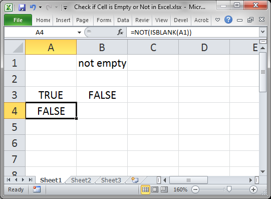
Use the ISBLANK() function.

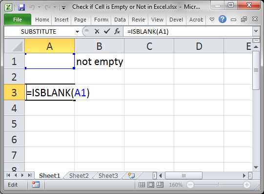
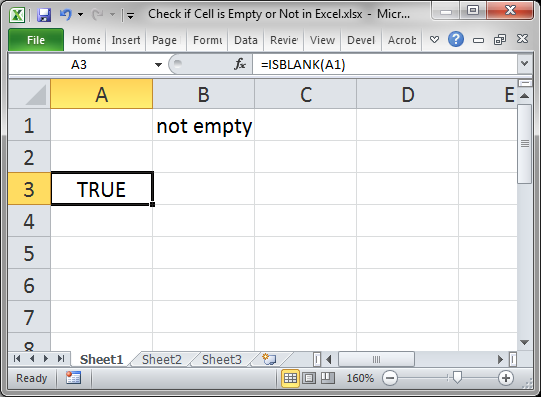
This will return TRUE if the cell is empty or FALSE if the cell is not empty.

Here, cell A1 is being checked, which is empty.

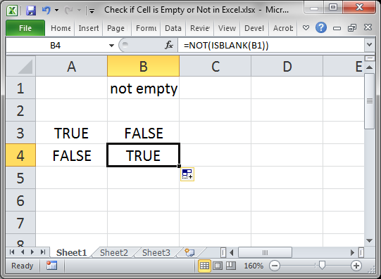
When the cell is not empty, it looks like this:

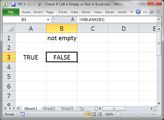
FALSE is output because cell B1 is not empty.

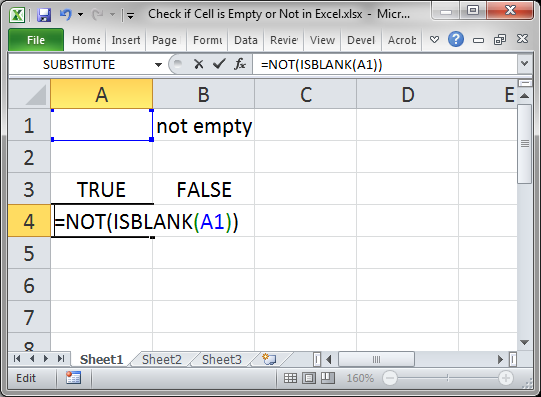
Reverse the True/False Output

Some formulas need to have TRUE or FALSE reversed in order to work correctly; to do this, use the NOT() function.

Result:

Whereas ISBLANK() output a TRUE for cell A1, the NOT() function reversed that and changed it to FALSE.

The same works for changing FALSE to TRUE.

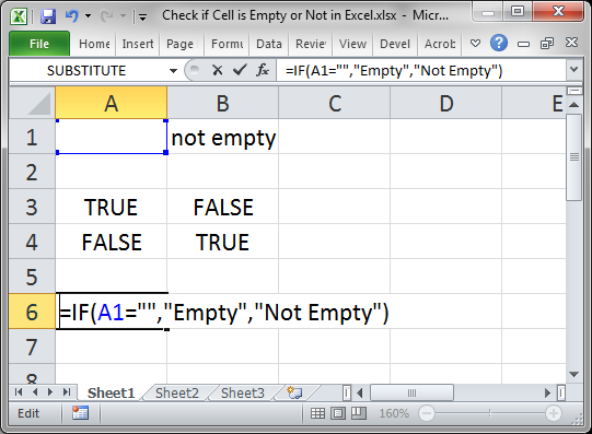
Check if a Cell is Empty or Not — Method 2

You can also use an IF statement to check if a cell is empty.

Result:

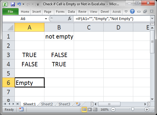
The function checks if this part is true: A1=»» which checks if A1 is equal to nothing.

When there is something in the cell, it works like this:

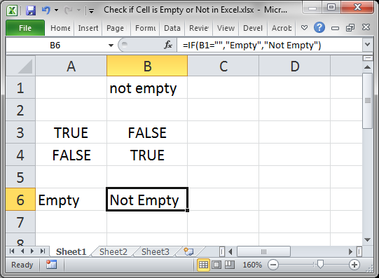
Cell B1 is not empty so we get a Not Empty result.

In this example I set the IF statement to output «Empty» or «Not Empty» but you can change it to whatever you like.

Reverse the Check

The example above checked if the cell was empty, but you can also check if the cell is not empty.

There are a few different ways to do this, but I will show you a simple and easy method here.

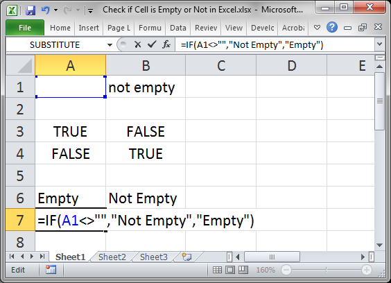
Notice the check this time is A1<>»» and that says «is cell A1 not equal to nothing.» It sounds confusing but just remember that <> is basically the reverse of =.

I also had to switch the «Empty» and «Not Empty» in order to get the correct result since we are now checking if the cell is not empty.

Result:

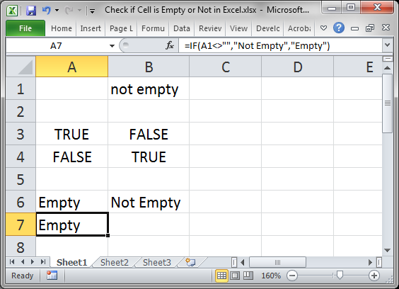
As you can see, it outputs the same result as the previous example, just like it should.

Using <> instead of = merely reverses it, making a TRUE become a FALSE and a FALSE become a TRUE, which is why «Empty» and «Not Empty» had to be reversed in order to still output the correct result.

Notes

It may seem useless to return TRUE or FALSE like in the first method, but remember that many functions in Excel, including IF(), AND(), and OR() all rely on results that are either TRUE or FALSE.

Checking for blanks and returning TRUE or FALSE is a simple concept but it can get a bit confusing in Excel, especially when you have complex formulas that rely on the result of the formulas in this tutorial. Save this tutorial and work with the attached sample file and you will have it down in no time.

Make sure to download the attached sample file to work with these examples in Excel.

Similar Content on TeachExcel

Odd or Even Row Formulas in Excel

Tutorial: Formulas to determine if the current cell is odd or even; this allows you to perform speci…

Subscribe for Weekly Tutorials

BONUS: subscribe now to download our Top Tutorials Ebook!

In this article, we will learn:

How To Check If A Cell Is Blank Using IF

How To Check If A Cell Is Blank Using ISBLANK

Count Blank Cells Using COUNTIF

Count Blank Cells Using COUNTBLANK

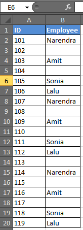
Assume you have this data.

Let’s just step into the example.

How To Check If A Cell Is Blank Using IF

Generic Formula

=IF(cell_address=»»,TRUE,FALSE)

In the above data, there are some names that are missing. In Column C you want TRUE if it doesn’t have a name and FALSE if it does. It is easy to do this. In C2 write this formula and copy it in the cells below.

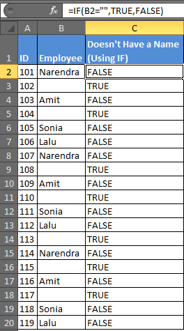
The formula simply checks to see if the cell is blank or not. It uses “”  to indicate blank. Prints TRUE  if it is blank, and FALSE if not.

How To Check If A Cell Is Blank Using ISBLANK

Generic Formula

Now the same task can be done easily by using the ISBLANKfunction in excel 2016.

ISBLANK takes only one argument and that is the cell you want to check.

In D2 write this formula and copy it below cells.

This will be your result.

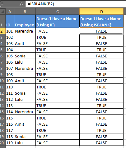
You got the same answers by giving just one argument in ISBLANK.

Mostly you would want to do something after knowing if the cell is blank or not. This is where IF is necessary.

For example, if you want to print the name Cells of B column has one, and “mystry_man” if it is a blank cell. You can use IF and ISBLANK in excel together.

In Range E2, write this formula:

Count Blank Cells Using COUNTIF

Generic Formula

Now if you want to know how many blank cells there are, you can use this formula.

In any version of Excel 2016, 2013, 2010, write this formula in any cell.

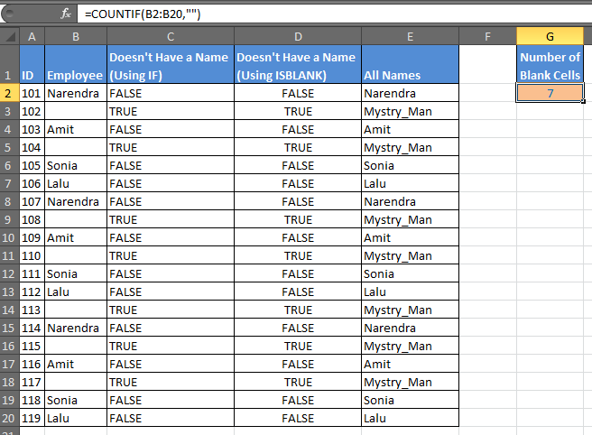
We have our answer as 7 for this example.

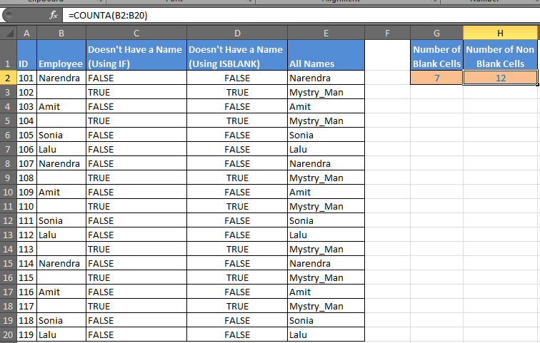
Now if you want to know how many names there are, you need to count if not blank. Use the COUNTA function to count non-blank cells in a range.

Count Blank Cells Using COUNTBLANK

Generic Formula

COUNTA counts if cell contains any text and the COUNTBLANK function counts all blank cells in a range in Excel. It only requires one argument to count empty cells in a range.

In cell G2, enter this formula:

COUNTBLANK will find blank cells in excel of the given range.

We learned how to work with blank cells in excel, how to find blank cells, how to count blank cells in a range, how to check if a cell is empty or not, how to manipulate blank cells etc.

Related Articles:

How to Calculate Only If Cell is Not Blank in Excel

Adjusting a Formula to Return a Blank

Checking Whether Cells in a Range are Blank, and Counting the Blank Cells

SUMIF with non-blank cells

Only Return Results from Non-Blank Cells

Popular Articles:

50 Excel Shortcuts to Increase Your Productivity

How to use the VLOOKUP Function in Excel

How to use the COUNTIF function in Excel

How to use the SUMIF Function in Excel

• #2

It isn’t clear whether you are looking for a worksheet formula or vba. A worksheet formula to find next non-empty row after A10 would be

=MATCH(TRUE,INDEX(A11:A100<>»»,0),0)+ROW(A10)

(I’m wondering what you are going to use that result for as there may be a more direct way to that next result.)

• #3

If you were looking for a UDF, you could try this. It returns the next non-empty row in the column or 0 if there is no subsequent non-empty cell in the column.
It assumes rStart is a single-cell range.

Code:

Function NextFilled(rStart As Range) As Long
  NextFilled = rStart.EntireColumn.Find(What:="?*", After:=rStart, LookIn:=xlValues).Row
  If NextFilled <= rStart.Row Then NextFilled = 0
End Function

Last edited: Apr 8, 2018

• #4

It isn’t clear whether you are looking for a worksheet formula or vba. A worksheet formula to find next non-empty row after A10 would be

=MATCH(TRUE,INDEX(A11:A100<>»»,0),0)+ROW(A10)

(I’m wondering what you are going to use that result for as there may be a more direct way to that next result.)

Thank you — and yes, I forgot to say that this is a UDF in VBA. What I need to do is, given a cell where there definitely IS a value, count down the number of cells in that column until a non-blank (not non-zero) cell is reached. I will have a go at converting your Excel code to VBA.

• #5

I will have a go at converting your Excel code to VBA.

Did you see post #3 ?

• #6

I did, but only after I’d posted. Your VBA code works well and I am busy integrating it into my application.
Thanks again. Much appreciated.

• #7

I did, but only after I’d posted. Your VBA code works well and I am busy integrating it into my application.
Thanks again. Much appreciated.

OK, great.

• #8

Hi @Peter_SSs. Thank so much for your continued assistance on this site.

I used the code as is and also modified it directly into a sub and worked both ways. One thing I wanted to ask is if you do not want to activate the sheet where you are seeking the NextFilled cell in a particular column, how can I change your code?

I tried the following and it gave me the error «Run-time error ’91’: Object variable or With block variable not set.»

VBA Code:

Function NextFilledF(ShtName As String, rStart As Range) As Long

    With Sheets(ShtName)       
            NextFilledF = rStart.EntireColumn.Find(What:="?*", After:=rStart, LookIn:=xlValues).Row
            If NextFilledF <= rStart.Row Then NextFilledF = 0
    End With
    

End Function

I believe the issue is that I need to set a with for the range rStart, but then how do I handle rStart within the line item? When I do the following I get the same error «Run-time error ’91’: Object variable or With block variable not set.»

VBA Code:

 Function NextFilledF(ShtName As String, rStart As Range) As Long

    With Sheets(ShtName)
        With rStart
            NextFilledF = .EntireColumn.Find(What:="?*", After:=rStart, LookIn:=xlValues).Row
            If NextFilledF <= rStart.Row Then NextFilledF = 0
        End With
    End With
    
End Function

• #9

If you are using a function, how exactly are you using it in a workbook?
Or else can you upload a small dummy file with no sensitive data and with the failing function used in it to DropBox, One Drive, Google Drive etc and post a publicly shared link here?

• #10

If you are using a function, how exactly are you using it in a workbook?
Or else can you upload a small dummy file with no sensitive data and with the failing function used in it to DropBox, One Drive, Google Drive etc and post a publicly shared link here?

Thanks @Peter_SSs for your response. I am trying to avoid activating the sheet as I would like to create a universal function whenever I need it in the future. Here is an example, with a summarized version of the code. I tested it and I get the error «»Run-time error ’91’: Object variable or With block variable not set.»

VBA Code:

Sub NextCellwValue()

'Dimensioning
    Dim NextFilled As Long
    Dim ShtName As String
    Dim Rng As Range
    Dim rStart As Range
  
  
'Code
    Sheets("SUMMARY").Activate
  
    ShtName = "DATA1"
    Set Rng = Range("A:A")
    Set rStart = Range("A7")
    NextFilled = NextFilledF(ShtName, Rng, rStart)
    Range("A1").Value = ShtName
    Range("B1").Value = NextFilled
  
    ShtName = "DATA2"
    Set Rng = Range("A:A")
    Set rStart = Range("A7")
    NextFilled = NextFilledF(ShtName, Rng, rStart)
    Range("A2").Value = ShtName
    Range("B2").Value = NextFilled


End Sub


'****************************************************************************************************
'This function find the next row of data in a range

Function NextFilledF(ShtName As String, Rng As Range, rStart As Range) As Long

    With Sheets(ShtName)
        With Rng.EntireColumn
            NextFilledF = .Find(What:="?*", After:=rStart, LookIn:=xlValues).Row
            If NextFilledF <= rStart.Row Then NextFilledF = 0
        End With
    End With
  
End Function