
In this tutorial, you will learn how to find Mode in excel with examples and simple steps. Thus we will describe different kinds of modes and use them in some instances.
Basically, we’ll describe first what is mode, thus organizations, and businesses use statistical data in decision-making and insights for their financial aspects
What is Mode?
Generally, a Mode is a frequently occurring number in a data set. A mode is simply a number that can easily find by counting how many times it occurs in a data set. Moreover, it is useful in statistical aspects which you can determine what is most popular item or rating in a survey, the most common grades students have.
Additionally, a data set can either have no mode, unimode ad two or more modes.
For example:
| Kind of Modes | Value |
| None | 1, 2, 3, 4, 6, 8, 9. |
| Unimodal: One mode found | 1, 2, 3, 3, 4, 5. |
| Bimodal: Two modes found | 1, 1, 2, 3, 4, 4, 5. |
| Trimodal: Three modes found | 1, 1, 2, 3, 3, 4, 5, 5. |
| Multimodal: More than one (two, three or more) | 1, 1, 2, 3, 3, 4, 5, 5, 7, 8, 9, 9 |
Note: Sometimes the mode is shortened to “mod”; Don’t confuse this with a calculus modulo function.
What is the mode function in Excel?
Excel’s mode function is similar to how it works in the median as measure of central tendency. For instance, in groups of numbers (5, 6, 7, 8, 9, 10) there is no mode because it frequently occurs once. Where in the set of numbers (10,10, 20, 30, 40) 10 is the mode because it appears twice.
Correspondingly, you may consider these several types of modes: No mode, Unimode, Bimodal, trimodal, and multimodal.
Another thing there are things to remember when using mode function in excel:
- #NUM! error – Happens if there are no duplicates; hence, there is no mode within the supplied values.
- #VALUE! error – Appears if a value supplied directly to the MODE is non-numeric and not part of an array. Non-numeric functions that are part of an array of values are ignored by the MODE function.
- In Excel 2010, the MODE.SNGL function replaced the MODE function. However, current versions of excel still have the Mode function in order to provide compatibility with earlier versions. However, it’s possible that MODE function will not be available in the future so better to learn and use MODE.SNGL.
Syntax
=MODE(number1,[number2],…)
MODE Function Syntax Arguments
number1: Required. The first number argument for which you want to calculate the mode.
number2, …: Optional. Number arguments 2 to 255 for which you want to calculate the mode. You can also use a single array or a reference to an array instead of arguments separated by commas.
To find the Mode in Microsoft Excel, you can apply referencing by constant values. Therefore you can write the function as:
=MODE(first number, second number, …)
So this formula explains that your mode is from the input number or values in the function specifically if your reference is like (1, 3, 3,4,6,7). Therefore the functions will return 3 as the mode because the number appears frequently.
In addition, if the data you input has unknown number of modes you can use the MODE.MULT function as follow:
=MODE.MULT(first number, second number, …)
Aside from calculating modes using constant value referencing, you can also use reference which is a range of cells. So can use the given formula below:
=MODE(cell name:cell name)
Considering this method, you can yield mode in your worksheet without inputting constant values. If you expect multiple modes, this method can also use MODE.MULT function. This displays multiple modes if a dataset has them in the cell you designate and the cells below it, and you might write it as follows:
=MODE.MULT(cell name:cell name)
how to find multiple modes in excel
To understand the uses of the MODE.MULT function, let’s consider a few examples:
Suppose we are given the following data:
The formula to use is:
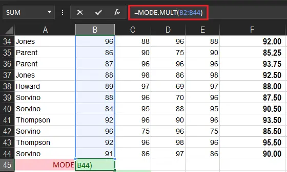
We get the result below:
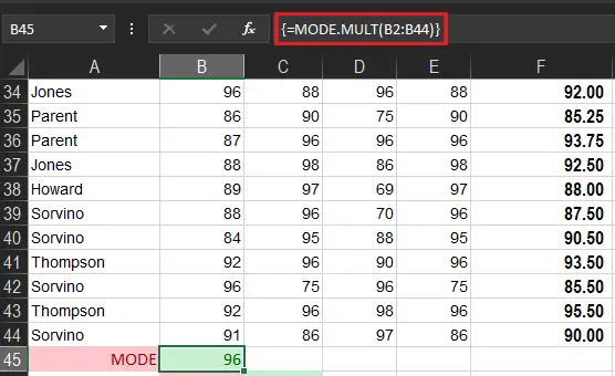
Note: The MODE.MULT function returns an array of results and must be entered as an array formula. To confirm the function Press Ctrl+Shift+Enter, to return each selected cell a mode value if it does not exist.
Average Function in Excel (Mean)
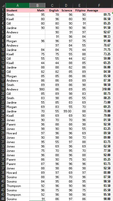
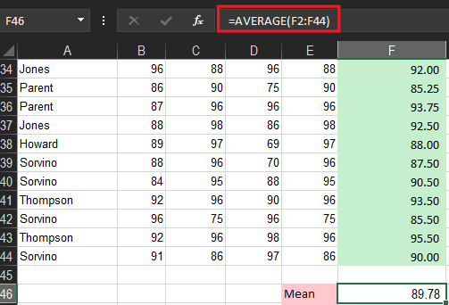
The average function in Excel is simple and often used especially in obtaining student grades. So, all you need to do is enter the formula and the range of cells. For instance the mean of the students below in their subjects.
Try this: =Average(F2:F44)
Median in Excel
The median function however is less complicated all you have to remember is when the given data set count is an odd number the middle value of the set is the median. On the other hand, if the data set count is even just get the average of the two middle values.
So we use =MEDIAN(F2:F44) to determine the median of the student average.
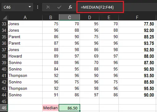
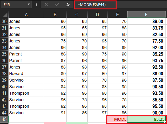
Mode in Excel
Meanwhile, if you want to know the element that occurs the most, the MODE function is a help. This is very crucial in working on a large amount of data and you want to know the frequently occurring value.
In our figure below, we use =MODE(F2:F44) and the mode of student average is 85.25.
Summary
In summary, finding mode in Excel is not that complicated. All you have to do is find the frequently appearing element on the data set. We hope you’ve learned and understood the concept of statistical function in Excel.
If you have more queries and suggestions regarding this topic, feel free to comment!
Excel for Microsoft 365 Excel for Microsoft 365 for Mac Excel for the web Excel 2021 Excel 2021 for Mac Excel 2019 Excel 2019 for Mac Excel 2016 Excel 2016 for Mac Excel 2013 Excel 2010 Excel 2007 Excel for Mac 2011 Excel Starter 2010 More…Less
Let’s say you want to find out the most common number of bird species sighted in a sample of bird counts at a critical wetland over a 30-year time period, or you want to find out the most frequently occurring number of phone calls at a telephone support center during off-peak hours. To calculate the mode of a group of numbers, use the MODE function.
MODE returns the most frequently occurring, or repetitive, value in an array or range of data.
Important: This function has been replaced with one or more new functions that may provide improved accuracy and whose names better reflect their usage. Although this function is still available for backward compatibility, you should consider using the new functions from now on, because this function may not be available in future versions of Excel.
For more information about the new functions, see MODE.MULT function and MODE.SNGL function.
Syntax
MODE(number1,[number2],…)
The MODE function syntax has the following arguments:
-
Number1 Required. The first number argument for which you want to calculate the mode.
-
Number2,… Optional. Number arguments 2 to 255 for which you want to calculate the mode. You can also use a single array or a reference to an array instead of arguments separated by commas.
Remarks
-
Arguments can either be numbers or names, arrays, or references that contain numbers.
-
If an array or reference argument contains text, logical values, or empty cells, those values are ignored; however, cells with the value zero are included.
-
Arguments that are error values or text that cannot be translated into numbers cause errors.
-
If the data set contains no duplicate data points, MODE returns the #N/A error value.
The MODE function measures central tendency, which is the location of the center of a group of numbers in a statistical distribution. The three most common measures of central tendency are:
-
Average which is the arithmetic mean, and is calculated by adding a group of numbers and then dividing by the count of those numbers. For example, the average of 2, 3, 3, 5, 7, and 10 is 30 divided by 6, which is 5.
-
Median which is the middle number of a group of numbers; that is, half the numbers have values that are greater than the median, and half the numbers have values that are less than the median. For example, the median of 2, 3, 3, 5, 7, and 10 is 4.
-
Mode which is the most frequently occurring number in a group of numbers. For example, the mode of 2, 3, 3, 5, 7, and 10 is 3.
For a symmetrical distribution of a group of numbers, these three measures of central tendency are all the same. For a skewed distribution of a group of numbers, they can be different.
Example
Copy the example data in the following table, and paste it in cell A1 of a new Excel worksheet. For formulas to show results, select them, press F2, and then press Enter. If you need to, you can adjust the column widths to see all the data.
|
Data |
||
|
5.6 |
||
|
4 |
||
|
4 |
||
|
3 |
||
|
2 |
||
|
4 |
||
|
Formula |
Description |
Result |
|
=MODE(A2:A7) |
Mode, or most frequently occurring number above |
4 |
Need more help?
Finding the mode (or “most often seen” value) of a set of numbers helps us to find the most likely outcome in a probability distribution. Microsoft Excel can find the mode for any set of values you choose as input.
So, how do you find mode in Excel? To find mode in Excel, use the “MODE” function. The input to the mode function is a range of cells (you can enter multiple cells, rows, columns, or blocks, separating inputs with a comma). For example, the mode of the values in cells A1 to A20 is given by the formula “=MODE(A1:A20)”.
Of course, there can be more than one mode for a data set in some case. Luckily, Excel also has more specific mode functions (MODE.SNGL and MODE.MULT) to deal with these cases.
In this article, we’ll talk about finding mode in Excel, including how to do it, alternative methods, and when you might use it. We’ll also look at some examples to make the concept clear.
Let’s get started.
The easiest way to find the mode (the most often seen or highest frequency value) in Excel is to use the “MODE” function. This function can take one or more inputs, separated by commas.
Each input is one or more cells – an input can be:
- a single cell (for example, “A1” would be a single cell)
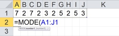
- a row (for example, “A1:J1” would be a row consisting of 10 cells)
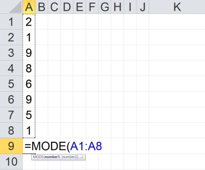
- a column (for example, “A1:A8” would be a column consisting of 8 cells)
- a block of cells (for example, “A1:J8” would be a block of cells consisting of 8 rows and 10 columns, for a total of 8*10 = 80 cells)
- a named range (for example “my_values”, which could denote any set of cells you choose, including an individual cell, a row, a column, or a block of cells)
For example, the mode of the values in cells A1 to J1 (a row of 10 cells) would be given by the formula
- =MODE(A1:J1)
You can see an example of this illustrated below.
The mode of the values in cells A1 to A8 (a column of 8 cells) would be given by the formula
- =MODE(A1:A8)
You can see an example of this illustrated below.
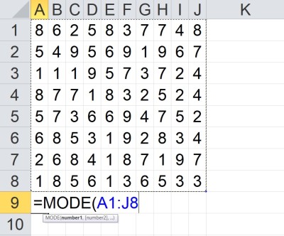
The mode of the values in cells A1 to J8 (a block of 80 cells) would be given by the formula
- =MODE(A1:J8)
You can see an example of this illustrated below.
The mode of the value in cells A1 to A5 and C1 to C5 would be given by the formula
- =MODE(A1:A5, C1:C5)
You can see an example of this illustrated below.
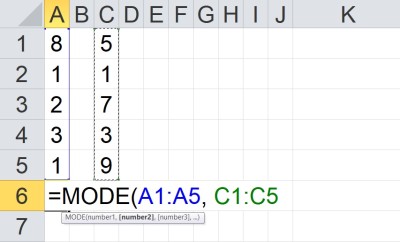
Note that the two inputs (A1:A5 and C1:C5) are separated by a comma. Each input has a total of 5 cells, for a total of 10 cells as input.
How Is Mode Calculated In Excel? (How Does Excel Find Mode)
MODE returns a single value (the highest frequency value) as an output. If two or more values are “tied” for highest frequency, then this function returns the smallest (minimum) of those values.
According to Microsoft Support:
“If the data set contains no duplicate data points, MODE returns the #N/A error value.”
https://support.microsoft.com/en-us/office/mode-function-e45192ce-9122-4980-82ed-4bdc34973120
In other words, if the frequency of every value in the data set is 1, the MODE function will return the error #N/A.
Excel needs to take a few steps to calculate the mode of a set of values (cells):
- First, make a list of all the unique values in the data set.
- Next, count how many times each unique value appears (that is, calculate the frequency for each unique value).
- If each value has a frequency of 1, return the “#N/A” error.
- Then, if there are multiple values with the highest frequency, use the minimum of the “tied” values as the mode. Otherwise, the highest frequency value is the mode.
Note that we can take the mode of any combination of cells, rows, columns, and blocks. The values don’t need to be in any particular order – the mode function will count the frequency for each value and find the “most often seen” one for us.
Note that MODE.SNGL and MODE.MULT work a little differently on the last step – you can learn more below.
MODE.SNGL vs MODE.MULT In Excel
More recent versions of Excel expand on the MODE function with two specialized functions. Both take the same inputs as MODE (as described above), but their outputs vary:
- MODE.SNGL returns a single value (the highest frequency value) as an output. If two or more values are “tied” for highest frequency, then this function returns the smallest (minimum) of those values.
- MODE.MULT returns a vertical array as an output. This vertical array contains all values of mode. If there is a single mode value, the array contains only one value – but if there are multiple values of mode, then the array contains all of them.
Note that for MODE.MULT to work properly, you must select a column of cells to contain the vertical array, enter the formula (=MODE.MULT(…)), and press “CTRL + SHIFT + ENTER”. This will return the vertical array of modes in the cells you originally selected.
Also note that if there are no repeated values in the data set, both of these functions will return the error #N/A (just as MODE does).
Here are two examples of how to find the mode of a data set in Excel – one using MODE.SNGL and one using MODE.MULT. We’ll start with MODE.SNGL.
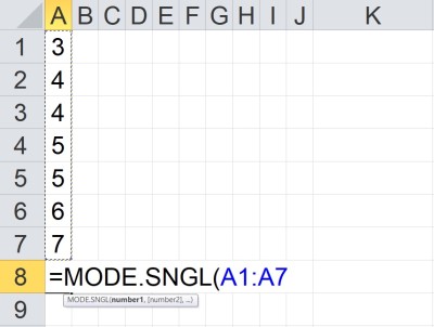
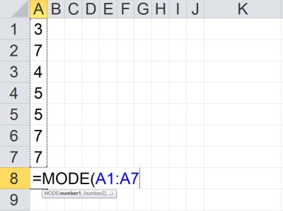
Example 1: Finding The Mode Using MODE.SNGL
Let’s say we want to take the mode of a set of the 7 values shown below:
- {3, 4, 4, 5, 5, 6, 7}
We can see that there are 5 unique values (3, 4, 5, 6, and 7), with counts as shown in the following table:
| Value | Frequency (Count) |
|---|---|
| 3 | 1 |
| 4 | 2* |
| 5 | 2* |
| 6 | 1 |
| 7 | 1 |
each unique value in the data set.
The counts for the values 4 and 5
have stars to indicate that they are
the highest frequency (modes).
This means that both 4 and 5 are tied for the highest frequency (both have a count of 2).
The MODE.SNGL function should take the minimum of these two values (4 and 5) to return 4. We can verify this below.
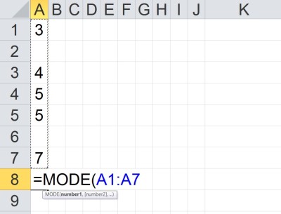
Example 2: Finding The Mode Using MODE.MULT
Let’s say we want to take the mode of a set of the 7 values shown below:
- {3, 4, 4, 5, 5, 6, 7}
We can see that there are 5 unique values (3, 4, 5, 6, and 7), with counts as shown in the following table:
| Value | Frequency (Count) |
|---|---|
| 3 | 1 |
| 4 | 2* |
| 5 | 2* |
| 6 | 1 |
| 7 | 1 |
each unique value in the data set.
The counts for the values 4 and 5
have stars to indicate that they are
the highest frequency (modes).
This means that both 4 and 5 are tied for the highest frequency (both have a count of 2).
The MODE.MULT function should return a vertical array containing both of these values (4 and 5) to return 4. We can verify this below.
As a reminder: remember that for MODE.MULT to work properly, you must select a column of cells to contain the vertical array, enter the formula (=MODE.MULT(…)), and press “CTRL + SHIFT + ENTER”. This will return the vertical array of modes in the cells you originally selected.
Below, we selected the cells A8 to A9, entered the formula “=MODE.MULT(A1:A7)”, and pressed “CTRL + SHIFT + ENTER”.

Does Mode In Excel Ignore Blank Cells?
Mode in Excel does ignore blanks. According to Microsoft Support:
“If an array or reference argument contains text, logical values, or empty cells, those values are ignored; however, cells with the value zero are included.”
If you wish to include blank cells in the mode calculation, then you must fill them in with some value (perhaps a value that does not appear in your list and is larger than all other values, so this “filler” value is not calculated to be the mode).
Example: Mode Function Ignores Blank Cells In Excel
If we take the mode of a column of 7 cells in Excel (two of which are blank), the blank cells are ignored (that is, they are not treated as zeroes or any other value).
You can see an example of this below:
However, if we fill in the two blank cells with values of 7, then we get a different mode, as shown below:
What Is The Meaning Of Mode In Excel?
Remember that mode is a measure of center. It helps us to get an idea of where the “middle” of a data set lies.
Mode tells us the highest frequency value in the data set (that is, the most often seen value). The mode also tells you the maximum (peak) value on a graph of the data.

A data set can have one, two, three, or more modes. Mode is not the same as mean or median, but they are equal in some cases.
You can learn more about what mode tells you about a data set here.
Why Is Mode Not Working In Excel?
According to Microsoft Support, there are several reasons that the MODE function is not working in Excel:
- One or more of the inputs (cells, rows, columns, blocks, named ranges) contains an error value (such as #N/A, etc.). If this is the case, try checking equations in those input cells to see where the errors are coming from.
- One or more of the inputs (cells, rows, columns, blocks, named ranges) contains text that cannot be translated into a number.
- The data set contains no duplicate data points (that is, the frequency of every data point is 1, and so every number is the most often seen, which means there is no mode).
If the MODE.MULT function is only returning one value when you know that it should be returning 2 or more in a vertical array, remember that for MODE.MULT to work properly, you must:
- select a column of cells to contain the vertical array
- enter the formula (=MODE.MULT(…))
- press “CTRL + SHIFT + ENTER”
This will return the vertical array of modes in the cells you originally selected.
Conclusion
Now you know how to find mode in Excel, as well as the uses of the alternative functions MODE.SNGL and MODE.MULT.
You can learn more about mode and other descriptive statistics here.
You can learn how to find mean in Excel here.
You can learn how to find median in Excel here.
Today, we’ll learn to find the median and mode in Excel. In statistics, the median is the value that separates the upper and lower halves of a data sample or population or simply the middle number in a sorted list of numbers. Excel has an inbuilt function MEDIAN to find the median value of a dataset.
Also read: How to calculate mean in Excel? [Easy Step-by-Step Method]
Using the MEDIAN function
The MEDIAN function returns the median of a list of numbers. Syntax: =MEDIAN(n), where n is the list of numbers or reference to the cell ranges containing the numbers.
Let us consider a list of numbers whose median we are interested in calculating:

- Go to the cell where you want to display the median value.
- Type =MEDIAN(, select the cells containing the numbers and complete the formula with ).

- Press Enter key to display the calculated median value.

Note:
- The Excel MEDIAN function returns the middle number in the dataset when the total number of items is odd. It returns the average of the two middle numbers when the total number of items in the dataset is even.
- In calculating median using the MEDIAN function, cells with values as zero (0) are included.
- The MEDIAN function ignores empty cells as well as cells containing text or logical values.
- TRUE and FALSE logical values put directly into the MEDIAN function’s parameters are counted as 1 and 0 respectively. The formula MEDIAN(FALSE, TRUE,2,3,4), returns 2 as the dataset is read as {0,1,2,3,4}.
Using the MEDIAN IF formula
Sometimes you want to exclude zero values while calculating the median of a dataset. Excel does not have a dedicated function to do this, but a workaround is available using a MEDIAN IF formula. The syntax for this formula is MEDIAN(IF(criteria_range=criteria, cell_ranges)), where criteria are the condition to be satisfied by the values in the cells, cell_ranges is the reference to the cell ranges containing the values.
Let us consider a list of numbers whose median we are interested in calculating excluding zero values:

- Go to the cell where you want to display the median value.
- Type =MEDIAN(IF(A1:A10>0,A1:A10)).

- Press Enter key to display the calculated median value of the numbers excluding zero values.

To illustrate the difference in the median, we calculated the mean of the above dataset including zeroes.

As you can see, the median is different in both cases.
Finding mode in Excel
The mode is a statistical term that refers to the most frequently occurring number found in a set of numbers. A data set can have none, one, or multiple modes. In Excel, there are three functions to find the mode/modes of a dataset which are discussed below:
Using the MODE function
This function returns a single mode. Syntax: MODE(n), where n is the list of numbers or reference to the cell ranges containing the numbers. Follow these steps to find the mode of a dataset using the MODE function:
- Go to the cell where you want to display the mode value.
- Type =MODE(, select the cells containing the numbers and complete the formula with ).

- Press Enter key to display the result.

Note:
- If the data set contains no data value that has at least one duplicate value, the MODE function returns the #N/A error value.
- The MODE function ignores empty cells as well as cells containing text or logical values.
Using the MODE.MULT function
This function returns more than one result if there are multiple modes in the dataset. Syntax: MODE.MULT(n), where n is the list of numbers or reference to the cell ranges containing the numbers. Follow these steps to find the Mode of a dataset using the MODE.MULT function:
- Go to the cell where you want to display the mode value.
- Type =MODE.MULT(, select the cells containing the numbers and complete the formula with ).

- Press Enter key to display the result.

Note:
- If the data set contains no data value that has at least one duplicate value, the MODE.MULT function returns the #N/A error value.
- The MODE.MULT function ignores empty cells as well as cells containing text or logical values.
Using the MODE.SNGL function
This function is an advanced version of the MODE function and returns a single most frequently occurring value in a dataset. Syntax: MODE.SNGL(n), where n is the list of numbers or reference to the cell ranges containing the numbers. Follow these steps to find the mode of a dataset using the MODE.SNGL function:
- Go to the cell where you want to display the mode value.
- Type =MODE.SNGL(, select the cells containing the numbers and complete the formula with ).

- Press the Enter key to display the result.

Note:
- If the data set contains no data value that has at least one duplicate value, the MODE.SNGL function returns the #N/A error value.
- The MODE.SNGL function ignores empty cells as well as cells containing text or logical values.
Conclusion
We discussed simple and quick ways of calculating the median and the mode of a dataset in Excel.
Use a function to find the mode in Microsoft Excel
- Step 1: Type your data into one column.
- Step 2: Click a blank cell anywhere on the worksheet and then type “=MODE.
- Step 3: Change the range in Step 2 to reflect your actual data.
- Step 4: Press “Enter.” Excel will return the solution in the cell with the formula.
Contents
- 1 What is the formula for mode in Excel?
- 2 How do you manually calculate mode in Excel?
- 3 What is the mode formula?
- 4 How do I get Excel out of Calculate mode?
- 5 What does F9 do in Excel?
- 6 What if there is no mode?
- 7 How do you find the mode example?
- 8 What is mode formula with example?
- 9 How do I change my formula mode to automatic?
- 10 How do I permanently enable iterative in Excel?
- 11 What does Alt F11 do in Excel?
- 12 What does Alt F5 do in Excel?
- 13 What is Alt F8?
- 14 Can zero be a mode?
- 15 Does mode always exist?
- 16 What is the formula of mode Class 10?
- 17 What are the 3 types of mode?
- 18 What if there are 3 modes?
- 19 How do you find the mode of the following data?
What is the formula for mode in Excel?
The Excel MODE function returns the most frequently occurring number in a numeric data set. For example, =MODE(1,2,4,4,5,5,5,6) returns 5. A number representing the mode. number1 – A number or cell reference that refers to numeric values.
How do you manually calculate mode in Excel?
Click “Formulas” in the list of items on the left. In the Calculation options section, click the “Manual” radio button to turn on the ability to manually calculate each worksheet. When you select “Manual”, the “Recalculate workbook before saving” check box is automatically checked.
What is the mode formula?
What is h in Mode Formula? In the mode formula,Mode = L+h(fm−f1)(fm−f1)−(fm−f2) L + h ( f m − f 1 ) ( f m − f 1 ) − ( f m − f 2 ) , h refers to the size of the class interval.
How do I get Excel out of Calculate mode?
To set the calculation mode to manual, proceed to the Ribbon, select the Formulas tab and then find the Calculation grouping on the tab. Click on the Calculation Options button and select you guessed it Manual. To turn it back on, select Automatic.
What does F9 do in Excel?
F9. Calculates the workbook. By default, any time you change a value, Excel automatically calculates the workbook. Turn on Manual calculation (on the Formulas tab, in the Calculation group, click Calculations Options, Manual) and change the value in cell A1 from 5 to 6.
What if there is no mode?
There is no mode when all observed values appear the same number of times in a data set. There is more than one mode when the highest frequency was observed for more than one value in a data set.
How do you find the mode example?
Mode: The most frequent number—that is, the number that occurs the highest number of times. Example: The mode of {4 , 2, 4, 3, 2, 2} is 2 because it occurs three times, which is more than any other number.
What is mode formula with example?
For example, The mode of Set A = {2,2,2,3,4,4,5,5,5} is 2 and 5, because both 2 and 5 is repeated three times in the given set.
How do I change my formula mode to automatic?
In the Excel for the web spreadsheet, click the Formulas tab. Next to Calculation Options, select one of the following options in the dropdown: To recalculate all dependent formulas every time you make a change to a value, formula, or name, click Automatic. This is the default setting.
How do I permanently enable iterative in Excel?
Learn about iterative calculation
- If you’re using Excel 2010 or later, click File > Options > Formulas.
- In the Calculation options section, select the Enable iterative calculation check box.
- To set the maximum number of times that Excel will recalculate, type the number of iterations in the Maximum Iterations box.
What does Alt F11 do in Excel?
F11 Creates a chart of the data in the current range in a separate Chart sheet. Shift+F11 inserts a new worksheet. Alt+F11 opens the Microsoft Visual Basic For Applications Editor, in which you can create a macro by using Visual Basic for Applications (VBA).
What does Alt F5 do in Excel?
h) Alt + Ctrl + Shift + F4: “Alt + Ctrl + Shift + F4” keys closes all open Excel file i.e. these work similar to “Alt + F4” keys. “F5” key is used to display “Go To” dialog box; it will help you in viewing named range. This will restore windows size of the current excel workbook.
What is Alt F8?
Alt+F8: Displays the Macro dialog box to create, run, edit, or delete a macro.(Pressing Alt does the same thing.)
Can zero be a mode?
Since the most frequently occuring value is zero (0) therefore zero (0) is the mode of the data set.For example, mean, median and mode of the standard normal distribution are all zero.
Does mode always exist?
Explanation: Mode is an item that occurs more number of times in a distribution.In an Individual Observation, if each item occurs only once, you will not get mode. In a Discrete Distribution and Continuous Distribution, there is mode always.
What is the formula of mode Class 10?
h = size of the class interval (assuming all class sizes to be equal), f1 = frequency of the modal class, f0 = frequency of the class preceding the modal class, f2 = frequency of the class succeeding the modal class.
What are the 3 types of mode?
The different types of mode are unimodal, bimodal, trimodal, and multimodal.
What if there are 3 modes?
A set of numbers with two modes is bimodal, a set of numbers with three modes is trimodal, and any set of numbers with more than one mode is multimodal.
How do you find the mode of the following data?
To find the mode, or modal value, it is best to put the numbers in order. Then count how many of each number. A number that appears most often is the mode.