Find lists in excel

Итог: Изучите быстрый и простой способ поиска любого списка проверки данных или раскрывающегося списка в ячейке с помощью бесплатного инструмента.

Уровень мастерства: Начинающий

Списки проверки данных являются отличным способом управления значениями, которые вводятся в ячейку. Эти выпадающие списки также позволяют нам выбирать параметры, которые могут управлять финансовыми моделями, отчетами или информационными панелями.

• Вы можете найти мой полный учебник по настройке списков проверки данных здесь.
• Тогда вы можете узнать, как сделать их динамичными здесь.
• И вы можете узнать, как сделать их зависимыми друг от друга здесь.

Тем не менее, нет встроенного способа поиска в списке
проверки в Excel. Пролистать эти списки может быть сложно, если в
раскрывающемся списке много элементов. Есть несколько действительно классных
решений на основе формул для этой проблемы, но они требуют большой работы по
настройке для каждого списка проверки в вашем файле.

Поэтому я разработал очень простую надстройку, которая
помогает решить эту проблему …

Нажмите на ссылки ниже, чтобы перейти к видео с обновлениями функции.

• Ноябрь 2016 Обновление
• Апрель 2017 Обновление

Поиск списков проверки с помощью поиска по списку

Надстройка поиска по списку позволяет быстро и легко
выполнять поиск в любом списке проверки. Он также работает со списками данных,
которые не содержат ячейки проверки данных.

Форма поиска
по списку содержит раскрывающийся список, в который загружается список проверки
выбранной ячейки. Раскрывающийся список также функционирует как окно поиска. Вы
можете ввести поиск в поле, и результаты будут сужаться по мере ввода. Это
Google-подобный поиск, и в результаты будет входить любой элемент, содержащий
поисковый запрос. Элемент не должен начинаться с поискового запроса.

После
того, как вы выбрали нужный элемент, нажмите клавишу «Ввод» на клавиатуре или
нажмите кнопку «Ввод значения» в форме, чтобы ввести значение в выбранную
ячейку.

Поиск по списку работает в любой ячейке любой книги. Никаких специальных настроек не требуется. Просто выберите ячейку, нажмите кнопку поиска и начните поиск по списку.

Параметры и функции поиска в списке

Надстройка
поиска по списку содержит некоторые функции, которые позволяют очень быстро
вводить данные и работать со списками. Нажмите кнопку меню в окне поиска по
списку, чтобы просмотреть параметры.

• Select Next Cell— после нажатия клавиши «Ввод» или «Ввод значения» выбирается ячейка под активной ячейкой. Это поведение можно изменить в раскрывающемся меню направления.
  • Down — выбирает ячейку под активной ячейкой.
  • Right — выбор ячейки справа от активной ячейки.
  • None — не меняет выбор.
  • Close — закрывает окно поиска по списку.
  • Paste — копирует входное значение в буфер обмена и вставляет его в активную ячейку с помощью метода VBA SendKeys. Окно поиска по списку закрывается. Это единственная опция, которая сохраняет историю отмен в Excel.
• Sort Order — выпадающий список можно отсортировать по возрастанию (A-Z), по убыванию (Z-A) или оригинальному порядку, нажимая кнопки переключения в меню параметров. Это только сортирует список в окне поиска списка. Он не сортирует список проверки данных в ячейке.
• List Info — кнопка Info отображает дополнительную информацию о раскрывающемся списке. В настоящее время отображается общее количество элементов в списке.
• Create List of Unique Values — добавлена ​​новая кнопка, которая копирует содержимое раскрывающегося списка в буфер обмена. Затем вы можете вставить список в любой диапазон в рабочей книге. Это быстрый способ создания списка уникальных значений при использовании поиска по списку в ячейке, которая НЕ содержит проверки данных. Вы также можете отфильтровать список, введя поиск, а затем скопировать отфильтрованный список в буфер обмена.

ВАЖНО. Примечание.

При вводе значений в активную ячейку единственным способом сохранить историю отмен является использование параметра «Вставить» в раскрывающемся списке «Выбрать следующую ячейку». Поиск по списку использует макросы для ввода выбранного значения, и макросы обычно очищают историю отмен в Excel, когда они изменяют книгу.

Параметр Вставить — это обходной путь, который использует метод SendKeys для копирования и вставки выбранного значения. Это имитирует то, что пользователь будет делать для копирования / вставки, и НЕ очищает историю отмен в Excel.

Работает со списками без проверки данных

Поиск по
списку работает в ячейках, которые также не содержат проверки данных. Если вы
выберете ячейку, которая НЕ содержит проверку данных, и откроете Поиск по
списку, в раскрывающемся списке будет загружен список уникальных элементов из
столбца выбранной ячейки.

Это похоже на нажатие Alt + Стрелка вниз в ячейке, чтобы увидеть список значений в этом столбце. Тем не менее, список не должен быть непрерывным. Даже если столбец содержит пробелы, Поиск по списку все равно загрузит все уникальные значения в текущей области данных или списке.

Ноябрь 2016 Обновление

Я
опубликовал обновленную версию надстройки поиска по списку с несколькими новыми
функциями. Вот видео обзор новых функций.

Вот список возможностей:

1. Добавлена ​​опция «Вставить» в список
   направлений. Это скопирует входное значение в буфер обмена и вставит его в
   активную ячейку. Параметры Paste используют метод SendKeys в VBA для выполнения
   вставки. Это означает, что история отмен не будет очищена при использовании
   опции вставки.
2. Настройки для меню параметров и раскрывающегося
   списка направления ввода теперь сохраняются в реестре. Ваши настройки будут
   сохранены и загружены при следующем открытии Excel и надстройки.
3. Добавлены улучшения для таблиц Excel. Когда
   активная ячейка находится в таблице, а ячейка не содержит проверки, будет
   загружен уникальный список значений, исключая заголовки таблицы и итоговую
   строку.
4. Добавлена ​​функция копирования списка, которая
   копирует содержимое выпадающего списка в буфер обмена. Эта функция используется
   для создания списка уникальных значений из столбца / таблицы, когда активная
   ячейка не содержит проверки. Это также работает, когда список фильтруется
   поисковым запросом, чтобы копировать только отфильтрованные результаты.

Апрель 2017 Обновление

Исходя из
ваших потрясающих отзывов и запросов, я рад опубликовать еще одно обновление с
новыми функциями. Я делюсь новыми возможностями в следующем видео.

Вот список новых функций в обновлении апреля 2017 года:

1. Он добавил функцию автоматического открытия,
   чтобы автоматически открывать форму, когда выбрана ячейка, содержащая проверку
   данных. Вы можете включить или отключить эту опцию с помощью
   кнопки-переключателя в меню параметров.
2. Теперь надстройка работает с проверкой данных,
   созданной с помощью формул (OFFSET
   & INDEX) и
   разделенных запятыми списков. Он должен работать со всеми типами списков
   проверки данных.
3. Обновлено поведение клавиши Escape, чтобы закрыть окно поиска по
   списку. Если в окне поиска есть текст, Escape очищает окно поиска. Если поле поиска пустое, Escape закрывает форму.

В видео я
также показал несколько ячеек с иконками раскрывающихся кнопок рядом с ними,
хотя эта ячейка не была выбрана. Посмотрите мою статью о том, как сделать так,
чтобы выпадающие кнопки списка проверки
всегда были видны, чтобы узнать больше об этой технике.

Загрузите надстройку поиска по списку (это бесплатно!)

Надстройка поиска списка бесплатна для загрузки и использования. Код VBA также имеет открытый исходный код, поэтому вы можете изменить его для своих нужд. Это также отличный способ узнать, как работают макросы и надстройки, если вы изучаете VBA.

Примечание. Вы
создадите бесплатную учетную запись на сайте участников Excel Campus для доступа к загрузке
и любым последующим обновлениям.

Сайт загрузки также содержит инструкции по установке и
видео.

Как мои коллеги могут использовать поиск по списку?

Надстройка поиска по списку установлена ​​на вашем
компьютере, и только вы сможете увидеть вкладку XL Campus и использовать поиск
по списку. Если вы хотите, чтобы ваши коллеги могли использовать Поиск по
списку, есть два способа сделать это.

1. Отправьте им ссылку на эту страницу, чтобы загрузить и установить Поиск по списку на своем компьютере. Они смогут использовать Поиск по списку в любом файле Excel, который они открыли на своем компьютере.
2. Импортируйте пользовательскую форму поиска по списку в проект VB в файле Excel. Вы можете добавить форму поиска по списку в любую из ваших книг. Это должна быть книга с макросами. Вам также потребуется создать или импортировать модуль кода, который содержит макрос, чтобы открыть пользовательскую форму поиска по списку. Затем добавьте кнопку на лист или ленту, которая открывает форму.

Как мы можем улучшить
поиск по списку?

Надеюсь, надстройка поиска по списку сэкономит вам время на поиск в списках проверки данных. Конечная цель состоит в том, чтобы быстрее находить искомое значение в длинных списках данных.

Пожалуйста, оставьте комментарий ниже с любыми вопросами или предложениями. Спасибо!

So, there are times when you would like to know that a value is in a list or not. We have done this using VLOOKUP. But we can do the same thing using COUNTIF function too. So in this article, we will learn how to check if a values is in a list or not using various ways.

Check If Value In Range Using COUNTIF Function

So as we know, using COUNTIF function in excel we can know how many times a specific value occurs in a range. So if we count for a specific value in a range and its greater than zero, it would mean that it is in the range. Isn’t it?

Generic Formula

=COUNTIF(range,value)>0

Range: The range in which you want to check if the value exist in range or not.

Value: The value that you want to check in the range.

Let’s see an example:

Excel Find Value is in Range Example

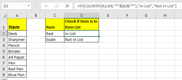
For this example, we have below sample data. We need a check-in the cell D2, if the given item in C2 exists in range A2:A9 or say item list. If it’s there then, print TRUE else FALSE.

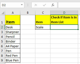
Write this formula in cell D2:

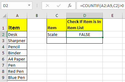
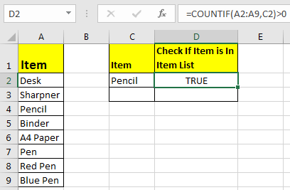
Since C2 contains “scale” and it’s not in the item list, it shows FALSE. Exactly as we wanted. Now if you replace “scale” with “Pencil” in the formula above, it’ll show TRUE.

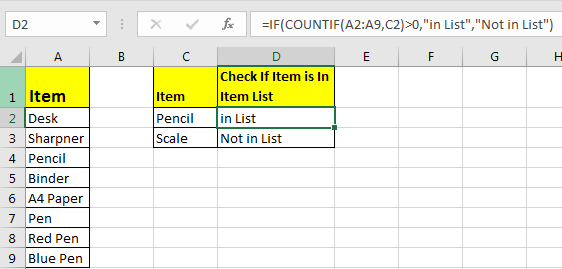
Now, this TRUE and FALSE looks very back and white. How about customizing the output. I mean, how about we show, “found” or “not found” when value is in list and when it is not respectively.
Since this test gives us TRUE and FALSE, we can use it with IF function of excel.

Write this formula:

=IF(COUNTIF(A2:A9,C2)>0,»in List»,»Not in List»)

You will have this as your output.

What If you remove “>0” from this if formula?

=IF(COUNTIF(A2:A9,C2),»in List»,»Not in List»)

It will work fine. You will have same result as above. Why? Because IF function in excel treats any value greater than 0 as TRUE.

How to check if a value is in Range with Wild Card Operators

Sometimes you would want to know if there is any match of your item in the list or not. I mean when you don’t want an exact match but any match.

For example, if in the above-given list, you want to check if there is anything with “red”. To do so, write this formula.

=IF(COUNTIF(A2:A9,»*red*»),»in List»,»Not in List»)

This will return a TRUE since we have “red pen” in our list. If you replace red with pink it will return FALSE. Try it.
Now here I have hardcoded the value in list but if your value is in a cell, say in our favourite cell B2 then write this formula.

IF(COUNTIF(A2:A9,»*»&B2&»*»),»in List»,»Not in List»)

There’s one more way to do the same. We can use the MATCH function in excel to check if the column contains a value. Let’s see how.

Find if a Value is in a List Using MATCH Function

So as we all know that MATCH function in excel returns the index of a value if found, else returns #N/A error. So we can use the ISNUMBER to check if the function returns a number.
If it returns a number ISNUMBER will show TRUE, which means it’s found else FALSE, and you know what that means.

Write this formula in cell C2:

=ISNUMBER(MATCH(C2,A2:A9,0))

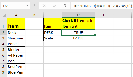
The MATCH function looks for an exact match of value in cell C2 in range A2:A9. Since DESK is on the list, it shows a TRUE value and FALSE for SCALE.

So yeah, these are the ways, using which you can find if a value is in the list or not and then take action on them as you like using IF function. I explained how to find value in a range in the best way possible. Let me know if you have any thoughts. The comments section is all yours.

Related Articles:

How to Check If Cell Contains Specific Text in Excel

How to Check A list of Texts In String in Excel

How to take the Average Difference between lists in Excel

How to Get Every Nth Value From A list in Excel

Popular Articles:

50 Excel Shortcuts to Increase Your Productivity

How to use the VLOOKUP Function in Excel

How to use the COUNTIF function in Excel

How to use the SUMIF Function in Excel

Let’s say that you want to look up an employee’s phone extension by using their badge number, or the correct rate of a commission for a sales amount. You look up data to quickly and efficiently find specific data in a list and to automatically verify that you are using correct data. After you look up the data, you can perform calculations or display results with the values returned. There are several ways to look up values in a list of data and to display the results.

What do you want to do?

• Look up values vertically in a list by using an exact match

• Look up values vertically in a list by using an approximate match

• Look up values vertically in a list of unknown size by using an exact match

• Look up values horizontally in a list by using an exact match

• Look up values horizontally in a list by using an approximate match

• Create a lookup formula with the Lookup Wizard (Excel 2007 only)

Look up values vertically in a list by using an exact match

To do this task, you can use the VLOOKUP function, or a combination of the INDEX and MATCH functions.

VLOOKUP examples

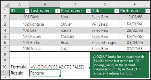
For more information, see VLOOKUP function.

INDEX and MATCH examples

In simple English it means:

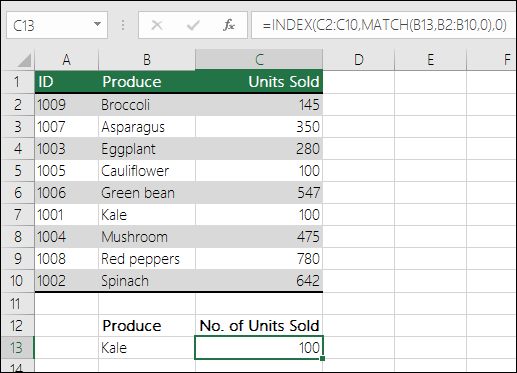
=INDEX(I want the return value from C2:C10, that will MATCH(Kale, which is somewhere in the B2:B10 array, where the return value is the first value corresponding to Kale))

The formula looks for the first value in C2:C10 that corresponds to Kale (in B7) and returns the value in C7 (100), which is the first value that matches Kale.

For more information, see INDEX function and MATCH function.

Top of Page

Look up values vertically in a list by using an approximate match

To do this, use the VLOOKUP function.

Important:  Make sure the values in the first row have been sorted in an ascending order.

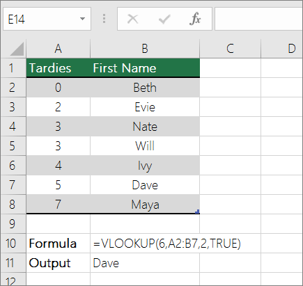
In the above example, VLOOKUP looks for the first name of the student who has 6 tardies in the A2:B7 range. There is no entry for 6 tardies in the table, so VLOOKUP looks for the next highest match lower than 6, and finds the value 5, associated to the first name Dave, and thus returns Dave.

For more information, see VLOOKUP function.

Top of Page

Look up values vertically in a list of unknown size by using an exact match

To do this task, use the OFFSET and MATCH functions.

Note: Use this approach when your data is in an external data range that you refresh each day. You know the price is in column B, but you don’t know how many rows of data the server will return, and the first column isn’t sorted alphabetically.

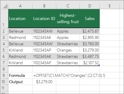
C1 is the upper left cells of the range (also called the starting cell).

MATCH(«Oranges»,C2:C7,0) looks for Oranges in the C2:C7 range. You should not include the starting cell in the range.

1 is the number of columns to the right of the starting cell where the return value should be from. In our example, the return value is from column D, Sales.

Top of Page

Look up values horizontally in a list by using an exact match

To do this task, use the HLOOKUP function. See an example below:

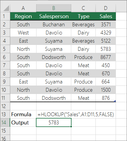
HLOOKUP looks up the Sales column, and returns the value from row 5 in the specified range.

For more information, see HLOOKUP function.

Top of Page

Look up values horizontally in a list by using an approximate match

To do this task, use the HLOOKUP function.

Important:  Make sure the values in the first row have been sorted in an ascending order.

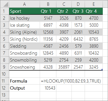
In the above example, HLOOKUP looks for the value 11000 in row 3 in the specified range. It does not find 11000 and hence looks for the next largest value less than 1100 and returns 10543.

For more information, see HLOOKUP function.

Top of Page

Create a lookup formula with the Lookup Wizard (Excel 2007 only)

Note: The Lookup Wizard add-in was discontinued in Excel 2010. This functionality has been replaced by the function wizard and the available Lookup and reference functions (reference).

In Excel 2007, the Lookup Wizard creates the lookup formula based on a worksheet data that has row and column labels. The Lookup Wizard helps you find other values in a row when you know the value in one column, and vice versa. The Lookup Wizard uses INDEX and MATCH in the formulas that it creates.

1. Click a cell in the range.

2. On the Formulas tab, in the Solutions group, click Lookup.

3. If the Lookup command is not available, then you need to load the Lookup Wizard add-in program.

   How to load the Lookup Wizard Add-in program

4. Click the Microsoft Office Button , click Excel Options, and then click the Add-ins category.

5. In the Manage box, click Excel Add-ins, and then click Go.

6. In the Add-Ins available dialog box, select the check box next to Lookup Wizard, and then click OK.

7. Follow the instructions in the wizard.

Top of Page

Mazzaropi


Posts

1983

Registration date
Monday August 16, 2010
Status
Contributor
Last seen
February 27, 2023

146

Mar 7, 2017 at 09:57 AM

Priya, Good morning.

Suppose:

List_One.xlsx

Sheet1

A1:A1000 —> huge list of names

B1:B1000 —> FORMULA

List_Two.xlsx

Sheet1

A1:A200 —> List of names

Try to use:

List_One.xlsx

Sheet1

B1 —> =IF(ISNUMBER(MATCH(A1, [List_Two.xlsx]Sheet1!$A$1:$A$200, 0 )), «-ok-«, «— NOT FOUND —«)

Copy it down as necessary.

Is that what you want?

I hope it helps.

—

Belo Horizonte, Brasil.

Marcílio Lobão