Find in excel spreadsheet - Word и Excel - помощь в работе с программами

Содержание

Поиск данных в таблице или диапазоне ячеек с помощью встроенных функций Excel
Описание
Создание образца листа
Определения терминов
Функции
LOOKUP ()
INDEX () и MATCH ()
СМЕЩ () и MATCH ()
Use Excel built-in functions to find data in a table or a range of cells
Summary
Create the Sample Worksheet
Term Definitions
Functions
LOOKUP()
VLOOKUP()
INDEX() and MATCH()
OFFSET() and MATCH()
SEARCH, SEARCHB functions
Description
Syntax
Remark
Examples

Поиск данных в таблице или диапазоне ячеек с помощью встроенных функций Excel

Примечание: Мы стараемся как можно оперативнее обеспечивать вас актуальными справочными материалами на вашем языке. Эта страница переведена автоматически, поэтому ее текст может содержать неточности и грамматические ошибки. Для нас важно, чтобы эта статья была вам полезна. Просим вас уделить пару секунд и сообщить, помогла ли она вам, с помощью кнопок внизу страницы. Для удобства также приводим ссылку на оригинал (на английском языке).

Описание

В этой статье приведены пошаговые инструкции по поиску данных в таблице (или диапазоне ячеек) с помощью различных встроенных функций Microsoft Excel. Для получения одного и того же результата можно использовать разные формулы.

Создание образца листа

В этой статье используется образец листа для иллюстрации встроенных функций Excel. Рассматривайте пример ссылки на имя из столбца A и возвращает возраст этого человека из столбца C. Чтобы создать этот лист, введите указанные ниже данные в пустой лист Excel.

Введите значение, которое вы хотите найти, в ячейку E2. Вы можете ввести формулу в любую пустую ячейку на том же листе.

Определения терминов

В этой статье для описания встроенных функций Excel используются указанные ниже условия.

Вся таблица подстановки

Значение, которое будет найдено в первом столбце аргумента «инфо_таблица».

Просматриваемый_массив
-или-
Лукуп_вектор

Диапазон ячеек, которые содержат возможные значения подстановки.

Номер столбца в аргументе инфо_таблица, для которого должно быть возвращено совпадающее значение.

3 (третий столбец в инфо_таблица)

Ресулт_аррай
-или-
Ресулт_вектор

Диапазон, содержащий только одну строку или один столбец. Он должен быть такого же размера, что и просматриваемый_массив или Лукуп_вектор.

Логическое значение (истина или ложь). Если указано значение истина или опущено, возвращается приближенное соответствие. Если задано значение FALSE, оно будет искать точное совпадение.

Это ссылка, на основе которой вы хотите основать смещение. Топ_целл должен ссылаться на ячейку или диапазон смежных ячеек. В противном случае функция СМЕЩ возвращает #VALUE! значение ошибки #ИМЯ?.

Число столбцов, находящегося слева или справа от которых должна указываться верхняя левая ячейка результата. Например, значение «5» в качестве аргумента Оффсет_кол указывает на то, что верхняя левая ячейка ссылки состоит из пяти столбцов справа от ссылки. Оффсет_кол может быть положительным (то есть справа от начальной ссылки) или отрицательным (то есть слева от начальной ссылки).

Функции

LOOKUP ()

Функция Просмотр находит значение в одной строке или столбце и сопоставляет его со значением в той же позицией в другой строке или столбце.

Ниже приведен пример синтаксиса формулы подСТАНОВКи.

= Просмотр (искомое_значение; Лукуп_вектор; Ресулт_вектор)

Следующая формула находит возраст Марии на листе «образец».

= ПРОСМОТР (E2; A2: A5; C2: C5)

Формула использует значение «Мария» в ячейке E2 и находит слово «Мария» в векторе подстановки (столбец A). Формула затем соответствует значению в той же строке в векторе результатов (столбец C). Так как «Мария» находится в строке 4, функция Просмотр возвращает значение из строки 4 в столбце C (22).

Примечание. Для функции Просмотр необходимо, чтобы таблица была отсортирована.

Чтобы получить дополнительные сведения о функции Просмотр , щелкните следующий номер статьи базы знаний Майкрософт:

Функция ВПР или вертикальный просмотр используется, если данные указаны в столбцах. Эта функция выполняет поиск значения в левом столбце и сопоставляет его с данными в указанном столбце в той же строке. Функцию ВПР можно использовать для поиска данных в отсортированных или несортированных таблицах. В следующем примере используется таблица с несортированными данными.

Ниже приведен пример синтаксиса формулы ВПР :

= ВПР (искомое_значение; инфо_таблица; номер_столбца; интервальный_просмотр)

Следующая формула находит возраст Марии на листе «образец».

= ВПР (E2; A2: C5; 3; ЛОЖЬ)

Формула использует значение «Мария» в ячейке E2 и находит слово «Мария» в левом столбце (столбец A). Формула затем совпадет со значением в той же строке в Колумн_индекс. В этом примере используется «3» в качестве Колумн_индекс (столбец C). Так как «Мария» находится в строке 4, функция ВПР возвращает значение из строки 4 В столбце C (22).

Чтобы получить дополнительные сведения о функции ВПР , щелкните следующий номер статьи базы знаний Майкрософт:

INDEX () и MATCH ()

Вы можете использовать функции индекс и ПОИСКПОЗ вместе, чтобы получить те же результаты, что и при использовании поиска или функции ВПР.

Ниже приведен пример синтаксиса, объединяющего индекс и Match для получения одинаковых результатов поиска и ВПР в предыдущих примерах:

= Индекс (инфо_таблица; MATCH (искомое_значение; просматриваемый_массив; 0); номер_столбца)

Следующая формула находит возраст Марии на листе «образец».

= ИНДЕКС (A2: C5; MATCH (E2; A2: A5; 0); 3)

Формула использует значение «Мария» в ячейке E2 и находит слово «Мария» в столбце A. Затем он будет соответствовать значению в той же строке в столбце C. Так как «Мария» находится в строке 4, формула возвращает значение из строки 4 в столбце C (22).

Обратите внимание Если ни одна из ячеек в аргументе «число» не соответствует искомому значению («Мария»), эта формула будет возвращать #N/А.
Чтобы получить дополнительные сведения о функции индекс , щелкните следующий номер статьи базы знаний Майкрософт:

СМЕЩ () и MATCH ()

Функции СМЕЩ и ПОИСКПОЗ можно использовать вместе, чтобы получить те же результаты, что и функции в предыдущем примере.

Ниже приведен пример синтаксиса, объединяющего смещение и сопоставление для достижения того же результата, что и функция Просмотр и ВПР.

= СМЕЩЕНИЕ (топ_целл, MATCH (искомое_значение; просматриваемый_массив; 0); Оффсет_кол)

Эта формула находит возраст Марии на листе «образец».

= СМЕЩЕНИЕ (A1; MATCH (E2; A2: A5; 0); 2)

Формула использует значение «Мария» в ячейке E2 и находит слово «Мария» в столбце A. Формула затем соответствует значению в той же строке, но двум столбцам справа (столбец C). Так как «Мария» находится в столбце A, формула возвращает значение в строке 4 в столбце C (22).

Чтобы получить дополнительные сведения о функции СМЕЩ , щелкните следующий номер статьи базы знаний Майкрософт:

Источник

Use Excel built-in functions to find data in a table or a range of cells

Summary

This step-by-step article describes how to find data in a table (or range of cells) by using various built-in functions in Microsoft Excel. You can use different formulas to get the same result.

Create the Sample Worksheet

This article uses a sample worksheet to illustrate Excel built-in functions. Consider the example of referencing a name from column A and returning the age of that person from column C. To create this worksheet, enter the following data into a blank Excel worksheet.

You will type the value that you want to find into cell E2. You can type the formula in any blank cell in the same worksheet.

Term Definitions

This article uses the following terms to describe the Excel built-in functions:

The whole lookup table

The value to be found in the first column of Table_Array.

Lookup_Array
-or-
Lookup_Vector

The range of cells that contains possible lookup values.

The column number in Table_Array the matching value should be returned for.

3 (third column in Table_Array)

Result_Array
-or-
Result_Vector

A range that contains only one row or column. It must be the same size as Lookup_Array or Lookup_Vector.

A logical value (TRUE or FALSE). If TRUE or omitted, an approximate match is returned. If FALSE, it will look for an exact match.

This is the reference from which you want to base the offset. Top_Cell must refer to a cell or range of adjacent cells. Otherwise, OFFSET returns the #VALUE! error value.

This is the number of columns, to the left or right, that you want the upper-left cell of the result to refer to. For example, «5» as the Offset_Col argument specifies that the upper-left cell in the reference is five columns to the right of reference. Offset_Col can be positive (which means to the right of the starting reference) or negative (which means to the left of the starting reference).

Functions

LOOKUP()

The LOOKUP function finds a value in a single row or column and matches it with a value in the same position in a different row or column.

The following is an example of LOOKUP formula syntax:

The following formula finds Mary’s age in the sample worksheet:

The formula uses the value «Mary» in cell E2 and finds «Mary» in the lookup vector (column A). The formula then matches the value in the same row in the result vector (column C). Because «Mary» is in row 4, LOOKUP returns the value from row 4 in column C (22).

NOTE: The LOOKUP function requires that the table be sorted.

For more information about the LOOKUP function, click the following article number to view the article in the Microsoft Knowledge Base:

VLOOKUP()

The VLOOKUP or Vertical Lookup function is used when data is listed in columns. This function searches for a value in the left-most column and matches it with data in a specified column in the same row. You can use VLOOKUP to find data in a sorted or unsorted table. The following example uses a table with unsorted data.

The following is an example of VLOOKUP formula syntax:

The following formula finds Mary’s age in the sample worksheet:

The formula uses the value «Mary» in cell E2 and finds «Mary» in the left-most column (column A). The formula then matches the value in the same row in Column_Index. This example uses «3» as the Column_Index (column C). Because «Mary» is in row 4, VLOOKUP returns the value from row 4 in column C (22).

For more information about the VLOOKUP function, click the following article number to view the article in the Microsoft Knowledge Base:

INDEX() and MATCH()

You can use the INDEX and MATCH functions together to get the same results as using LOOKUP or VLOOKUP.

The following is an example of the syntax that combines INDEX and MATCH to produce the same results as LOOKUP and VLOOKUP in the previous examples:

The following formula finds Mary’s age in the sample worksheet:

The formula uses the value «Mary» in cell E2 and finds «Mary» in column A. It then matches the value in the same row in column C. Because «Mary» is in row 4, the formula returns the value from row 4 in column C (22).

NOTE: If none of the cells in Lookup_Array match Lookup_Value («Mary»), this formula will return #N/A.
For more information about the INDEX function, click the following article number to view the article in the Microsoft Knowledge Base:

OFFSET() and MATCH()

You can use the OFFSET and MATCH functions together to produce the same results as the functions in the previous example.

The following is an example of syntax that combines OFFSET and MATCH to produce the same results as LOOKUP and VLOOKUP:

This formula finds Mary’s age in the sample worksheet:

The formula uses the value «Mary» in cell E2 and finds «Mary» in column A. The formula then matches the value in the same row but two columns to the right (column C). Because «Mary» is in column A, the formula returns the value in row 4 in column C (22).

For more information about the OFFSET function, click the following article number to view the article in the Microsoft Knowledge Base:

Источник

SEARCH, SEARCHB functions

This article describes the formula syntax and usage of the SEARCH and SEARCHB functions in Microsoft Excel.

Description

The SEARCH and SEARCHB functions locate one text string within a second text string, and return the number of the starting position of the first text string from the first character of the second text string. For example, to find the position of the letter «n» in the word «printer», you can use the following function:

This function returns 4 because «n» is the fourth character in the word «printer.»

You can also search for words within other words. For example, the function

returns 5, because the word «base» begins at the fifth character of the word «database». You can use the SEARCH and SEARCHB functions to determine the location of a character or text string within another text string, and then use the MID and MIDB functions to return the text, or use the REPLACE and REPLACEB functions to change the text. These functions are demonstrated in Example 1 in this article.

These functions may not be available in all languages.

SEARCHB counts 2 bytes per character only when a DBCS language is set as the default language. Otherwise SEARCHB behaves the same as SEARCH, counting 1 byte per character.

The languages that support DBCS include Japanese, Chinese (Simplified), Chinese (Traditional), and Korean.

Syntax

The SEARCH and SEARCHB functions have the following arguments:

find_text Required. The text that you want to find.

within_text Required. The text in which you want to search for the value of the find_text argument.

start_num Optional. The character number in the within_text argument at which you want to start searching.

The SEARCH and SEARCHB functions are not case sensitive. If you want to do a case sensitive search, you can use FIND and FINDB.

You can use the wildcard characters — the question mark ( ?) and asterisk ( *) — in the find_text argument. A question mark matches any single character; an asterisk matches any sequence of characters. If you want to find an actual question mark or asterisk, type a tilde (

) before the character.

If the value of find_text is not found, the #VALUE! error value is returned.

If the start_num argument is omitted, it is assumed to be 1.

If start_num is not greater than 0 (zero) or is greater than the length of the within_text argument, the #VALUE! error value is returned.

Use start_num to skip a specified number of characters. Using the SEARCH function as an example, suppose you are working with the text string «AYF0093.YoungMensApparel». To find the position of the first «Y» in the descriptive part of the text string, set start_num equal to 8 so that the serial number portion of the text (in this case, «AYF0093») is not searched. The SEARCH function starts the search operation at the eighth character position, finds the character that is specified in the find_text argument at the next position, and returns the number 9. The SEARCH function always returns the number of characters from the start of the within_text argument, counting the characters you skip if the start_num argument is greater than 1.

Examples

Copy the example data in the following table, and paste it in cell A1 of a new Excel worksheet. For formulas to show results, select them, press F2, and then press Enter. If you need to, you can adjust the column widths to see all the data.

Источник

Purpose

Get location substring in a string

Return value

A number representing the location of substring

Usage notes

The FIND function returns the position (as a number) of one text string inside another. If there is more than one occurrence of the search string, FIND returns the position of the first occurrence. When the text is not found, FIND returns a #VALUE error. Also note, when find_text is empty, FIND returns 1. FIND does not support wildcards, and is always case-sensitive. Use the SEARCH function to find the position of text without case-sensitivity and with wildcard support.

Basic Example

The FIND function is designed to look inside a text string for a specific substring. When FIND locates the substring, it returns a position of the substring in the text as a number. If the substring is not found, FIND returns a #VALUE error. For example:

=FIND("p","apple") // returns 2
=FIND("z","apple") // returns #VALUE!

Note that text values entered directly into FIND must be enclosed in double-quotes («»).

Case-sensitive

The FIND function always case-sensitive:

=FIND("a","Apple") // returns #VALUE!
=FIND("A","Apple") // returns 1

TRUE or FALSE result

To force a TRUE or FALSE result, nest the FIND function inside the ISNUMBER function. ISNUMBER returns TRUE for numeric values and FALSE for anything else. If FIND locates the substring, it returns the position as a number, and ISNUMBER returns TRUE:

=ISNUMBER(FIND("p","apple")) // returns TRUE
=ISNUMBER(FIND("z","apple")) // returns FALSE

If FIND doesn’t locate the substring, it returns an error, and ISNUMBER returns FALSE.

Start number

The FIND function has an optional argument called start_num, that controls where FIND should begin looking for a substring. To find the first match of «the» in any combination of upper or lowercase, you can omit start_num, which defaults to 1:

=FIND("x","20 x 30 x 50") // returns 4

To start searching at character 5, enter 4 for start_num:

=FIND("x","20 x 30 x 50",5) // returns 9

Wildcards

The FIND function does not support wildcards. See the SEARCH function.

If cell contains

To return a custom result with the SEARCH function, use the IF function like this:

=IF(ISNUMBER(FIND(substring,A1)), "Yes", "No")

Instead of returning TRUE or FALSE, the formula above will return «Yes» if substring is found and «No» if not.

Notes

The FIND function returns the location of the first find_text in within_text.
The location is returned as the number of characters from the start.
Start_num is optional and defaults to 1.
FIND returns 1 when find_text is empty.
FIND returns #VALUE if find_text is not found.
FIND is case-sensitive but does not support wildcards.
Use the SEARCH function to find a substring with wildcards.

Источник

This Excel tutorial explains how to use the Excel FIND function with syntax and examples.

Description

The Microsoft Excel FIND function returns the location of a substring in a string. The search is case-sensitive.

The FIND function is a built-in function in Excel that is categorized as a String/Text Function. It can be used as a worksheet function (WS) in Excel. As a worksheet function, the FIND function can be entered as part of a formula in a cell of a worksheet.

If you want to follow along with this tutorial, download the example spreadsheet.

Download Example

Syntax

The syntax for the FIND function in Microsoft Excel is:

FIND( substring, string, [start_position] )

Parameters or Arguments

substring: The substring that you want to find.
string: The string to search within.
start_position: Optional. It is the position in string where the search will start. The first position is 1. If the start_position is not provided, the FIND function will start the search at the beginning of the string.

Returns

The FIND function returns a numeric value. The first position in the string is 1.
If the FIND function does not find a match, it will return a #VALUE! error.

Applies To

Excel for Office 365, Excel 2019, Excel 2016, Excel 2013, Excel 2011 for Mac, Excel 2010, Excel 2007, Excel 2003, Excel XP, Excel 2000

Type of Function

Worksheet function (WS)

Example (as Worksheet Function)

Let’s look at some Excel FIND function examples and explore how to use the FIND function as a worksheet function in Microsoft Excel:

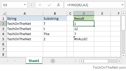
Based on the Excel spreadsheet above, the following FIND examples would return:

=FIND(B2,A2)
Result: 1

=FIND("T",A2)
Result: 1

=FIND("t",A3)
Result: 12

=FIND("The",A4)
Result: 7

=FIND("Z",A5)
Result: #VALUE!

=FIND("T", A2, 3)
Result: 7

Frequently Asked Questions

Question: In Microsoft Excel, I have the value «Supermarket» in cell A1 and 100 in cell A2.

Objective: If A1 contains «Super», then I want A3=A2. Otherwise, I want A3=0. I’m unable to use the FIND function because if cell A1 does not contain «Super», the FIND function returns the #VALUE! error which does not let me sum column A.

Answer: To make sure that do not return any #VALUE! errors when using the FIND function, you need to also use the ISERROR function in your formula.

Let’s look at an example.

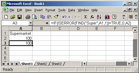
Based on the Excel spreadsheet above, the following FIND examples would return:

=IF(ISERROR(FIND("Super",A1,1))=TRUE,0,A2)
Result: 100

In this case, cell A1 does contain the value «Super», so the formula returns the value found in cell A2 which is 100.

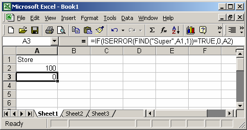
Based on the Excel spreadsheet above, the following FIND examples would return:

=IF(ISERROR(FIND("Super",A1,1))=TRUE,0,A2)
Result: 0

In this example, cell A1 does NOT contain the value «Super», so the formula returns 0.

Let’s just quickly explain how this formula works. If cell A1 contains «Super», the FIND function will return the numerical position of the value of «Super». Thus, an error will not result (ie. the IsError function evaluates to FALSE) and the formula will return A2.

If cell A1 does NOT contain «Super», the FIND function will return the #VALUE! error causing the IsError function to evaluate to TRUE and return 0.

Источник

Searching a Microsoft Excel spreadsheet may seem easy. While Ctrl + F can help you find most things in a spreadsheet, you’ll want to use more sophisticated tools to find and extract data based on specific values. We’ll help you save tons of time with our list of advanced search functions.

Once you know how to search in Excel using lookup, it won’t matter how big your spreadsheets get, you’ll always be able to find what you need!

1. The VLOOKUP Function

The VLOOKUP function lets you find a specific value within a column and extract values from the corresponding row in adjoining columns. Two examples where you might do this are (1) looking up an employee’s last name by their employee number, or (2) finding a phone number by specifying the last name.

Here’s the syntax of the function:

 =VLOOKUP([lookup_value], [table_array], [col_index_num], [range_lookup])

[lookup_value] is the piece of information that you already have. For example, if you need to know what state a city is in, it would be the name of the city.
[table_array] lets you specify the cells in which the function will look for the lookup and return values. When selecting your range, be sure that the first column included in your array is the one that will include your lookup value!
[col_index_num] is the number of the column that contains the return value.
[range_lookup] is an optional argument, and takes 1 or 0, though you could also enter TRUE or FALSE. If you enter 1 or omit this argument, the function looks for an approximate value, but we’ve found this to be hit-or-miss. In the example below, a VLOOKUP looking for a score of 100 returns 90. Looking for a lower value, for example 88, returned an error.

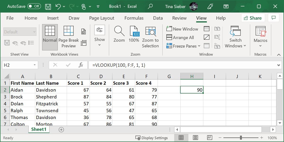
Let’s take a look at how you might use this. This spreadsheet contains student names and scores for four different tests. Let’s say you want to find score #4 for the student with the last name «Davidson.» VLOOKUP makes it easy.

Here’s the formula you’d use:

 =VLOOKUP("Davidson

Because the fourth score is the fifth column over from the last name we’re looking for, 5 is the column index argument. Note that when you’re looking for text, setting [range_lookup] to 0 is a good idea. Without it, you can get bad results.

Here’s the result:

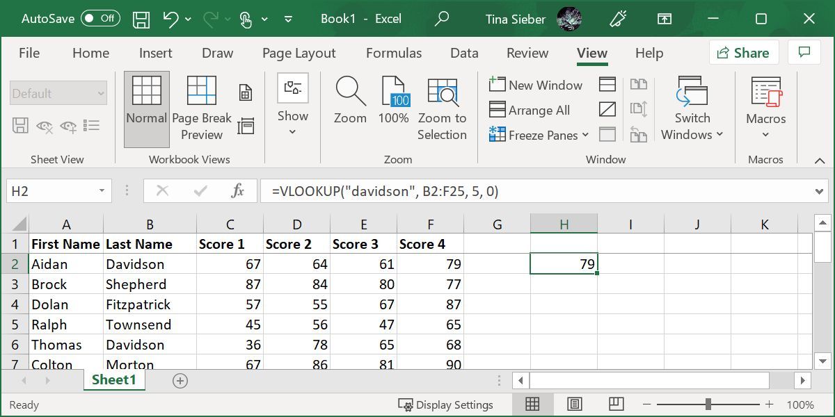
It returned 79, which is score #4 of the student we queried.

Notes on VLOOKUP

A few things are good to remember when you’re using VLOOKUP. Make sure that the first column in your range is the one that includes your lookup value. If it’s not in the first column, the function will return incorrect results. If your columns are well organized, this shouldn’t be a problem.

Also, keep in mind that VLOOKUP will only ever return one value. There was another student with the last name «Davidson,» but VLOOKUP will only ever return results for the first entry, with no indication that there is more than one match.

2. The HLOOKUP Function

Where VLOOKUP finds corresponding values in another column, HLOOKUP finds corresponding values in a different row. Because it’s usually easiest to scan through column headings until you find the right one and use a filter to find what you’re looking for, HLOOKUP is best used when you have huge spreadsheets, or if you’re working with values that are organized by time.

Here’s the syntax of the function:

 =HLOOKUP([lookup_value], [table_array], [row_index_num], [range_lookup])

[lookup_value] is the value that you know and want to find a corresponding value for.
[table_array] is the cells in which you want to search.
[row_index_num] specifies the row that the return value will come from.
[range_lookup] is the same as in VLOOKUP, leave it blank to get the nearest value when possible, or enter 0 to only look for exact matches.

We’ll use the same spreadsheet as before. You can use HLOOKUP to find the score for a specific row. Here’s how we’ll do it:

 =HLOOKUP("Score 4"

As you can see in the image below, the score is returned:

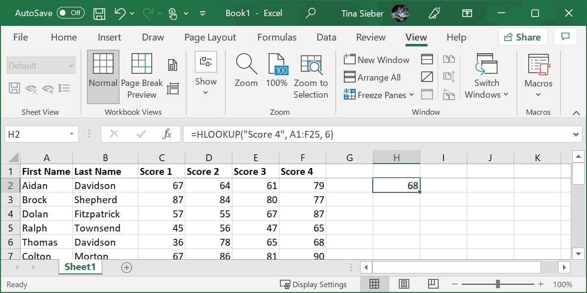
The student in row 6, Thomas Davidson, had a score of 68 on his fourth test.

Notes on HLOOKUP

As with VLOOKUP, the lookup value needs to be in the first row of your table array. This is rarely an issue with HLOOKUP, as you’ll usually be using a column title for a lookup value. HLOOKUP also only returns a single value.

3-4. The INDEX and MATCH Functions

INDEX and MATCH are two different functions, but when they’re used together, they can make searching a large spreadsheet a lot faster. Both functions have drawbacks, but by combining them, we’ll build on the strengths of both.

First, though, the syntax of both functions:

 =INDEX([array], [row_number], [column_number])

[array] is the array in which you’ll be searching.
[row_number] and [column_number] can be used to narrow your search (we’ll take a look at that in a moment).

 =MATCH([lookup_value], [lookup_array], [match_type])

[lookup_value] is a search term that can be a string or a number.
[lookup_array] is the array in which Microsoft Excel will look for the search term.
[match_type] is an optional argument that can be 1, 0, or -1. 1 will return the largest value that is smaller than or equal to your search term. 0 will only return your exact term, and -1 will return the smallest value that is greater than or equal to your search term.

It might not be clear how we’re going to use these two functions together, so I’ll lay it out here. MATCH takes a search term and returns a cell reference. In the image below, you can see that in a search for the last name «Davidson» in column B, MATCH returns 2.

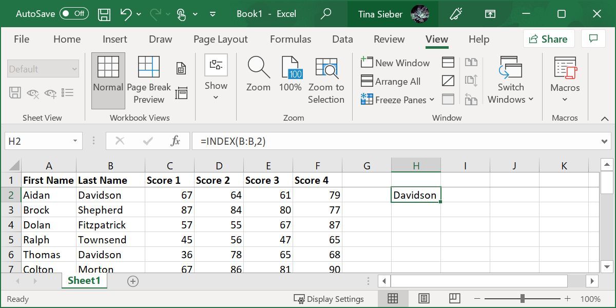
INDEX, on the other hand, does the opposite: it takes a cell reference and returns the value in it. You can see here that, when told to return the second row of column B, INDEX returns «Davidson,» the value from row 2.

What we’re going to do is combine the two so that MATCH returns a cell reference and INDEX uses that reference to look up the value in a cell. Let’s say you remember that there was a student whose last name was Townsend, and you want to see what this student’s fourth score was. Here’s the formula we’ll use:

 =INDEX(F:F, MATCH("Townsend", B:B, 0))

You’ll notice that the match type is set to 0 here. When you’re looking for a string, that’s what you’ll want to use. Here’s what we get when we run that function:

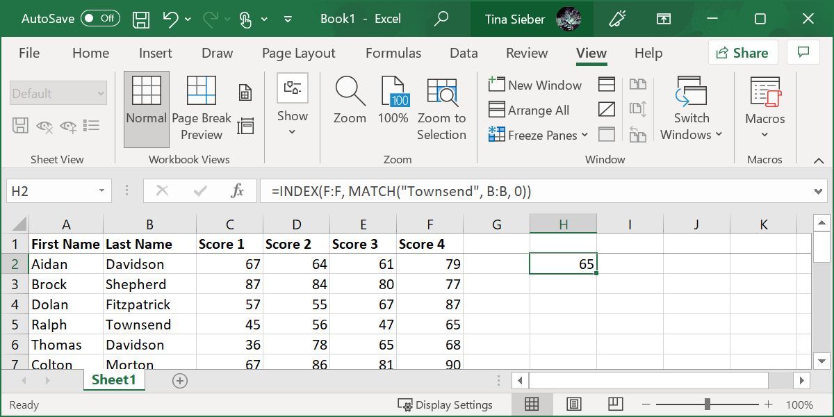
As you can see from the inset, Ralph Townsend scored a 68 in his fourth test, the number that appears when we run the function. This may not seem all that useful when you can just look a few columns over, but imagine how much time you’d save if you had to do it 50 times on a large database spreadsheet that contained several hundred columns!

5. The FIND Function

An article on finding something in Excel wouldn’t be complete without the FIND function. But it might not be what you expect. You can use Excel’s FIND function to identify the position of a string of text within another string of text.

Let’s say, we wanted to find the first occurrence of the letter «x» in the phrase «The brown fox jumped over the fence.» This would be our function:

 =FIND("x", "The brown fox jumped over the fence")

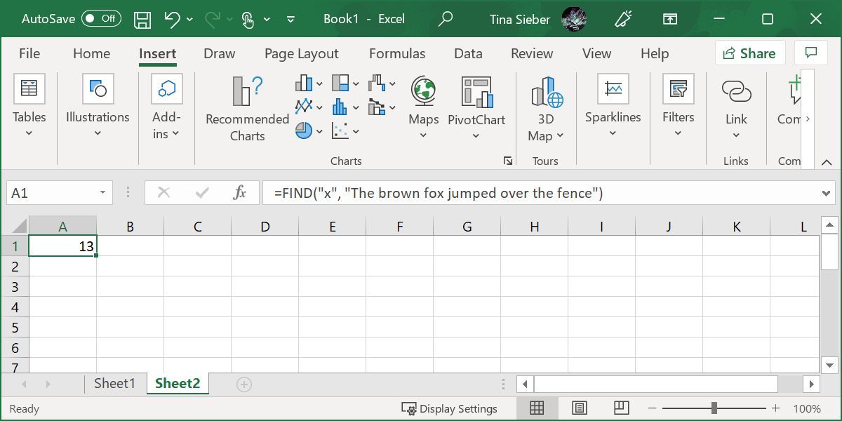
The resulting number represents the position of the queried string. If you’re looking for a multi-character string, let’s say we queried for «fox,» the result would indicate the position of the query’s first character; in this case 11.

Notes on FIND

Like VLOOKUP, HLOOKUP, and other functions, FIND will only identify the first occurrence of a string. Note that FIND is case-sensitive. You can use it to FIND multiple characters. And while we used a letter in our example, it also works with numbers.

On its own, this function might not seem very useful, but it comes into its own when you start nesting functions. For example, you could use your FIND result to split a string of text at the position corresponding to the string identified with FIND.

FIND vs. SEARCH

We can’t cover FIND without mentioning the SEARCH function. Well, it’s essentially the same as FIND, except that it’s not case-sensitive. It also allows wildcards, meaning you can search for matches that aren’t exact.

Excel supports three wildcards:

Asterisk (*), which is a placeholder for any number of characters, including zero.
Question mark (?), which can replace any one character.
Tilde (~), which turns the wildcards «asterisk» and «question mark» into literal characters, meaning it cancels their wildcard function. You’d use it as ~* or ~?.

6. The XLOOKUP Function

XLOOKUP is a new function designed to replace VLOOKUP. Like VLOOKUP, you can use it to find things in a table or range by searching for a known value. It differs from VLOOKUP in that it lets you look up values located in columns to the left or right of the queried value; with VLOOKUP you can only ever find data to the right of the queried column.

Here’s the syntax of the function:

=XLOOKUP(lookup_value, lookup_array, return_array, [if_not_found], [match_mode], [search_mode])

[lookup_value] is the value you’re searching for; i.e. your query.
[lookup_array] is the array or range to search.
[return_array] is the array or range to return. This is the first difference from VLOOKUP.
[if_not_found] is an optional argument that returns a message of your choice if no match is found.
[match_mode] is another optional argument that lets you find exact matches (0), the next smaller item (-1), the next larger item (1), or a wildcard match (2).
[search_mode] is optional and lets you control in which order to search. The default (1) starts the search at the first item. You can also start at the last item (-1), perform a binary search that depends on the lookup_array being sorted in ascending (2) or descending (-2) order.

Let’s take our VLOOKUP example and reverse the search order. This should let us find the score of the second student called Davidson. Here’s the formula:

 =XLOOKUP(G2,B2:B25,F2:F25,,,-1)

Note that we’re pulling the name from column G2, rather than writing it directly into the formula. Below is what it looks like.

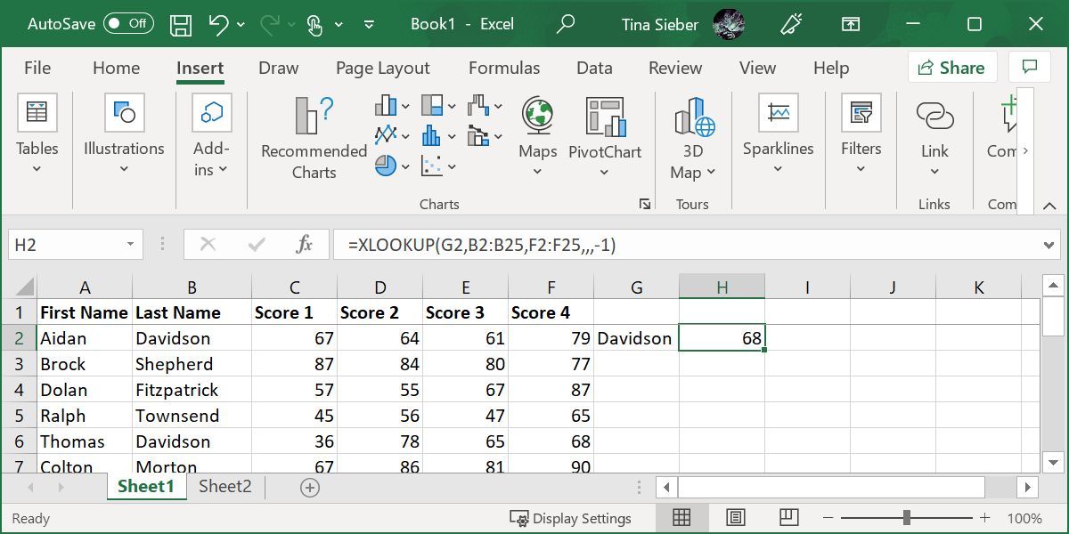
This time, the formula returned Thomas Davidson’s score, rather than that of Aidan Davidson. But it still can’t return more than one result.

Let the Excel Searches Begin

Microsoft Excel has a lot of extremely powerful functions for manipulating data, and the four listed above just scratch the surface. Learning how to use them will make your life much easier.

Источник