
See all How-To Articles
This tutorial demonstrates how to search all sheets to find a word or phrase in Excel and Google Sheets.
Search All Sheets
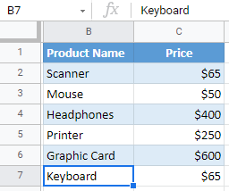
The search functionality in Excel searches in the current worksheet by default. However, you can also make it search all sheets in the file. Say you have the following Excel file with three sheets (January-2021, February-2021, and March-2021) and the same columns: Product Name and Price.
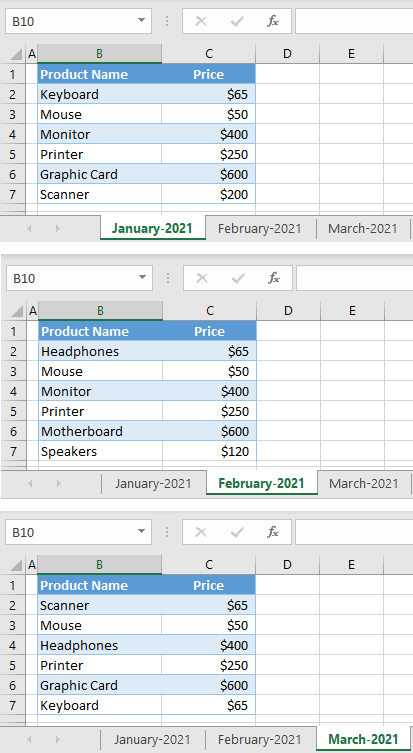
You want to search for Keyboard in the entire workbook. (It appears in cell B2 in sheet January-2021 and B7 in sheet March-2021.)
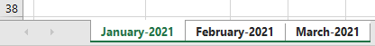
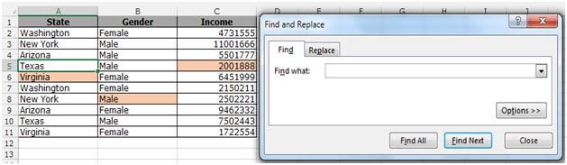
- First, select all sheets. Press and hold CTRL and click on sheet names (January-2021, February-2021, and March-2021.)
All sheets in the file are selected.
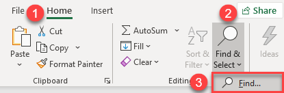
- In the Ribbon, go to Home > Find & Select > Find (or use the shortcut CTRL + F).
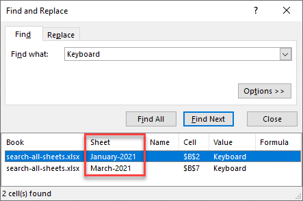
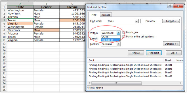
- Now, in the Find what box enter the word you want to find (“Keyboard“) and click Find All.
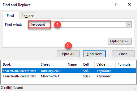
The bottom section of the window displays all appearances of the searched term in the workbook. As you can see, there are matches in the January-2021 (cell B2) and March-2021 (B7) sheets. If you click Find Next, you are cycled through each found cell.
See also: Using Find and Replace in Excel VBA
Search All Google Sheets
By default, Google Sheets searches all sheets for a term when you use Find and Replace.
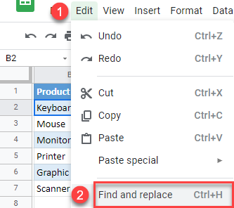
- In the Menu, go to Edit > Find and replace (or use the shortcut CTRL + H).
- In the Find box enter the word you want to find (“Keyboard“) and click Find.
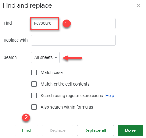
As a result, cell B2 in the January-2021 sheet is selected.
- Now when you click Find again, you go to the next instance of Keyboard (B7 in March-2021, and so on) through the last appearance of the term.
Unlike Excel, Google Sheets doesn’t offer the option to display a list of instances.
Содержание
- Use Excel built-in functions to find data in a table or a range of cells
- Summary
- Create the Sample Worksheet
- Term Definitions
- Functions
- LOOKUP()
- VLOOKUP()
- INDEX() and MATCH()
- OFFSET() and MATCH()
- How to Search All Sheets / Tabs in Excel & Google Sheets
- Search All Sheets
- Search All Google Sheets
- Поиск на листе Excel
- Поиск перебором значений
- Поиск функцией Find
- Примеры поиска функцией Find
- Поиск последней заполненной ячейки с помощью Find
- Поиск по шаблону (маске)
- Поиск в скрытых строках и столбцах
- Поиск даты с помощью Find
- Книги по теме:
- Посмотреть все книги по программированию
- Комментарии к статье:
Use Excel built-in functions to find data in a table or a range of cells
Summary
This step-by-step article describes how to find data in a table (or range of cells) by using various built-in functions in Microsoft Excel. You can use different formulas to get the same result.
Create the Sample Worksheet
This article uses a sample worksheet to illustrate Excel built-in functions. Consider the example of referencing a name from column A and returning the age of that person from column C. To create this worksheet, enter the following data into a blank Excel worksheet.
You will type the value that you want to find into cell E2. You can type the formula in any blank cell in the same worksheet.
Term Definitions
This article uses the following terms to describe the Excel built-in functions:
The whole lookup table
The value to be found in the first column of Table_Array.
Lookup_Array
-or-
Lookup_Vector
The range of cells that contains possible lookup values.
The column number in Table_Array the matching value should be returned for.
3 (third column in Table_Array)
Result_Array
-or-
Result_Vector
A range that contains only one row or column. It must be the same size as Lookup_Array or Lookup_Vector.
A logical value (TRUE or FALSE). If TRUE or omitted, an approximate match is returned. If FALSE, it will look for an exact match.
This is the reference from which you want to base the offset. Top_Cell must refer to a cell or range of adjacent cells. Otherwise, OFFSET returns the #VALUE! error value.
This is the number of columns, to the left or right, that you want the upper-left cell of the result to refer to. For example, «5» as the Offset_Col argument specifies that the upper-left cell in the reference is five columns to the right of reference. Offset_Col can be positive (which means to the right of the starting reference) or negative (which means to the left of the starting reference).
Functions
LOOKUP()
The LOOKUP function finds a value in a single row or column and matches it with a value in the same position in a different row or column.
The following is an example of LOOKUP formula syntax:
The following formula finds Mary’s age in the sample worksheet:
The formula uses the value «Mary» in cell E2 and finds «Mary» in the lookup vector (column A). The formula then matches the value in the same row in the result vector (column C). Because «Mary» is in row 4, LOOKUP returns the value from row 4 in column C (22).
NOTE: The LOOKUP function requires that the table be sorted.
For more information about the LOOKUP function, click the following article number to view the article in the Microsoft Knowledge Base:
VLOOKUP()
The VLOOKUP or Vertical Lookup function is used when data is listed in columns. This function searches for a value in the left-most column and matches it with data in a specified column in the same row. You can use VLOOKUP to find data in a sorted or unsorted table. The following example uses a table with unsorted data.
The following is an example of VLOOKUP formula syntax:
The following formula finds Mary’s age in the sample worksheet:
The formula uses the value «Mary» in cell E2 and finds «Mary» in the left-most column (column A). The formula then matches the value in the same row in Column_Index. This example uses «3» as the Column_Index (column C). Because «Mary» is in row 4, VLOOKUP returns the value from row 4 in column C (22).
For more information about the VLOOKUP function, click the following article number to view the article in the Microsoft Knowledge Base:
INDEX() and MATCH()
You can use the INDEX and MATCH functions together to get the same results as using LOOKUP or VLOOKUP.
The following is an example of the syntax that combines INDEX and MATCH to produce the same results as LOOKUP and VLOOKUP in the previous examples:
The following formula finds Mary’s age in the sample worksheet:
The formula uses the value «Mary» in cell E2 and finds «Mary» in column A. It then matches the value in the same row in column C. Because «Mary» is in row 4, the formula returns the value from row 4 in column C (22).
NOTE: If none of the cells in Lookup_Array match Lookup_Value («Mary»), this formula will return #N/A.
For more information about the INDEX function, click the following article number to view the article in the Microsoft Knowledge Base:
OFFSET() and MATCH()
You can use the OFFSET and MATCH functions together to produce the same results as the functions in the previous example.
The following is an example of syntax that combines OFFSET and MATCH to produce the same results as LOOKUP and VLOOKUP:
This formula finds Mary’s age in the sample worksheet:
The formula uses the value «Mary» in cell E2 and finds «Mary» in column A. The formula then matches the value in the same row but two columns to the right (column C). Because «Mary» is in column A, the formula returns the value in row 4 in column C (22).
For more information about the OFFSET function, click the following article number to view the article in the Microsoft Knowledge Base:
Источник
How to Search All Sheets / Tabs in Excel & Google Sheets
This tutorial demonstrates how to search all sheets to find a word or phrase in Excel and Google Sheets.
Search All Sheets
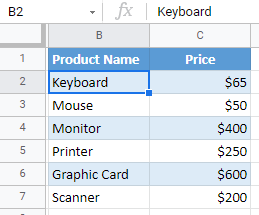
The search functionality in Excel searches in the current worksheet by default. However, you can also make it search all sheets in the file. Say you have the following Excel file with three sheets (January-2021, February-2021, and March-2021) and the same columns: Product Name and Price.
You want to search for Keyboard in the entire workbook. (It appears in cell B2 in sheet January-2021 and B7 in sheet March-2021.)
- First, select all sheets. Press and hold CTRL and click on sheet names (January-2021, February-2021, and March-2021.)
All sheets in the file are selected.
- In the Ribbon, go to Home > Find & Select > Find (or use the shortcut CTRL + F).
- Now, in the Find what box enter the word you want to find (“Keyboard“) and click Find All.
The bottom section of the window displays all appearances of the searched term in the workbook. As you can see, there are matches in the January-2021 (cell B2) and March-2021 (B7) sheets. If you click Find Next, you are cycled through each found cell.
Search All Google Sheets
By default, Google Sheets searches all sheets for a term when you use Find and Replace.
- In the Menu, go to Edit > Find and replace (or use the shortcut CTRL + H).
- In the Find box enter the word you want to find (“Keyboard“) and click Find.
As a result, cell B2 in the January-2021 sheet is selected.
- Now when you click Find again, you go to the next instance of Keyboard (B7 in March-2021, and so on) through the last appearance of the term.
Unlike Excel, Google Sheets doesn’t offer the option to display a list of instances.
Источник
Поиск на листе Excel

Поиск какого-либо значения в ячейках Excel довольно часто встречающаяся задача при программировании какого-либо макроса. Решить ее можно разными способами. Однако, в разных ситуациях использование того или иного способа может быть не оправданным. В данной статье я рассмотрю 2 наиболее распространенных способа.
Поиск перебором значений
Довольно простой в реализации способ. Например, найти в колонке «A» ячейку, содержащую «123» можно примерно так:
Минусами этого так сказать «классического» способа являются: медленная работа и громоздкость. А плюсом является его гибкость, т.к. таким способом можно реализовать сколь угодно сложные варианты поиска с различными вычислениями и т.п.
Поиск функцией Find
Гораздо быстрее обычного перебора и при этом довольно гибкий. В простейшем случае, чтобы найти в колонке A ячейку, содержащую «123» достаточно такого кода:
Вкратце опишу что делают строчки данного кода:
1-я строка: Выбираем в книге лист «Данные»;
2-я строка: Осуществляем поиск значения «123» в колонке «A», результат поиска будет в fcell;
3-я строка: Если удалось найти значение, то fcell будет содержать Range-объект, в противном случае — будет пустой, т.е. Nothing.
Полностью синтаксис оператора поиска выглядит так:
Find(What, After, LookIn, LookAt, SearchOrder, SearchDirection, MatchCase, MatchByte, SearchFormat)
What — Строка с текстом, который ищем или любой другой тип данных Excel
After — Ячейка, после которой начать поиск. Обратите внимание, что это должна быть именно единичная ячейка, а не диапазон. Поиск начинается после этой ячейки, а не с нее. Поиск в этой ячейке произойдет только когда весь диапазон будет просмотрен и поиск начнется с начала диапазона и до этой ячейки включительно.
LookIn — Тип искомых данных. Может принимать одно из значений: xlFormulas (формулы), xlValues (значения), или xlNotes (примечания).
LookAt — Одно из значений: xlWhole (полное совпадение) или xlPart (частичное совпадение).
SearchOrder — Одно из значений: xlByRows (просматривать по строкам) или xlByColumns (просматривать по столбцам)
SearchDirection — Одно из значений: xlNext (поиск вперед) или xlPrevious (поиск назад)
MatchCase — Одно из значений: True (поиск чувствительный к регистру) или False (поиск без учета регистра)
MatchByte — Применяется при использовании мультибайтных кодировок: True (найденный мультибайтный символ должен соответствовать только мультибайтному символу) или False (найденный мультибайтный символ может соответствовать однобайтному символу)
SearchFormat — Используется вместе с FindFormat. Сначала задается значение FindFormat (например, для поиска ячеек с курсивным шрифтом так: Application.FindFormat.Font.Italic = True), а потом при использовании метода Find указываем параметр SearchFormat = True. Если при поиске не нужно учитывать формат ячеек, то нужно указать SearchFormat = False.
Чтобы продолжить поиск, можно использовать FindNext (искать «далее») или FindPrevious (искать «назад»).
Примеры поиска функцией Find
Пример 1: Найти в диапазоне «A1:A50» все ячейки с текстом «asd» и поменять их все на «qwe»
Обратите внимание : Когда поиск достигнет конца диапазона, функция продолжит искать с начала диапазона. Таким образом, если значение найденной ячейки не менять, то приведенный выше пример зациклится в бесконечном цикле. Поэтому, чтобы этого избежать (зацикливания), можно сделать следующим образом:
Пример 2: Правильный поиск значения с использованием FindNext, не приводящий к зацикливанию.
В ниже следующем примере используется другой вариант продолжения поиска — с помощью той же функции Find с параметром After. Когда найдена очередная ячейка, следующий поиск будет осуществляться уже после нее. Однако, как и с FindNext, когда будет достигнут конец диапазона, Find продолжит поиск с его начала, поэтому, чтобы не произошло зацикливания, необходимо проверять совпадение с первым результатом поиска.
Пример 3: Продолжение поиска с использованием Find с параметром After.
Следующий пример демонстрирует применение SearchFormat для поиска по формату ячейки. Для указания формата необходимо задать свойство FindFormat.
Пример 4: Найти все ячейки с шрифтом «курсив» и поменять их формат на обычный (не «курсив»)
Примечание: В данном примере намеренно не используется FindNext для поиска следующей ячейки, т.к. он не учитывает формат (статья об этом: https://support.microsoft.com/ru-ru/kb/282151)
Коротко опишу алгоритм поиска Примера 4. Первые две строки определяют последнюю строку (lLastRow) на листе и последний столбец (lLastCol). 3-я строка задает формат поиска, в данном случае, будем искать ячейки с шрифтом Italic. 4-я строка определяет область ячеек с которой будет работать программа (с ячейки A1 и до последней строки и последнего столбца). 5-я строка осуществляет поиск с использованием SearchFormat. 6-я строка — цикл пока результат поиска не будет пустым. 7-я строка — меняем шрифт на обычный (не курсив), 8-я строка продолжаем поиск после найденной ячейки.
Хочу обратить внимание на то, что в этом примере я не стал использовать «защиту от зацикливания», как в Примерах 2 и 3, т.к. шрифт меняется и после «прохождения» по всем ячейкам, больше не останется ни одной ячейки с курсивом.
Свойство FindFormat можно задавать разными способами, например, так:
Поиск последней заполненной ячейки с помощью Find
Следующий пример — применение функции Find для поиска последней ячейки с заполненными данными. Использованные в Примере 4 SpecialCells находит последнюю ячейку даже если она не содержит ничего, но отформатирована или в ней раньше были данные, но были удалены.
Пример 5: Найти последнюю колонку и столбец, заполненные данными
В этом примере используется UsedRange, который так же как и SpecialCells возвращает все используемые ячейки, в т.ч. и те, что были использованы ранее, а сейчас пустые. Функция Find ищет ячейку с любым значением с конца диапазона.
Поиск по шаблону (маске)
При поиске можно так же использовать шаблоны, чтобы найти текст по маске, следующий пример это демонстрирует.
Пример 6: Выделить красным шрифтом ячейки, в которых текст начинается со слова из 4-х букв, первая и последняя буквы «т», при этом после этого слова может следовать любой текст.
Для поиска функцией Find по маске (шаблону) можно применять символы:
* — для обозначения любого количества любых символов;
? — для обозначения одного любого символа;
— для обозначения символов *, ? и
. (т.е. чтобы искать в тексте вопросительный знак, нужно написать
?, чтобы искать именно звездочку (*), нужно написать
* и наконец, чтобы найти в тексте тильду, необходимо написать
Поиск в скрытых строках и столбцах
Для поиска в скрытых ячейках нужно учитывать лишь один нюанс: поиск нужно осуществлять в формулах, а не в значениях, т.е. нужно использовать LookIn:=xlFormulas
Поиск даты с помощью Find
Если необходимо найти текущую дату или какую-то другую дату на листе Excel или в диапазоне с помощью Find, необходимо учитывать несколько нюансов:
- Тип данных Date в VBA представляется в виде #[месяц]/[день]/[год]#, соответственно, если необходимо найти фиксированную дату, например, 01 марта 2018 года, необходимо искать #3/1/2018#, а не «01.03.2018»
- В зависимости от формата ячеек, дата может выглядеть по-разному, поэтому, чтобы искать дату независимо от формата, поиск нужно делать не в значениях, а в формулах, т.е. использовать LookIn:=xlFormulas
Приведу несколько примеров поиска даты.
Пример 7: Найти текущую дату на листе независимо от формата отображения даты.
Пример 8: Найти 1 марта 2018 г.
Искать часть даты — сложнее. Например, чтобы найти все ячейки, где месяц «март», недостаточно искать «03» или «3». Не работает с датами так же и поиск по шаблону. Единственный вариант, который я нашел — это выбрать формат в котором месяц прописью для ячеек с датами и искать слово «март» в xlValues.
Тем не менее, можно найти, например, 1 марта независимо от года.
Пример 9: Найти 1 марта любого года.
Книги по теме:


Посмотреть все книги по программированию
Комментарии к статье:
| 10.09.17 Дмитрий | Очень толковая и полезная статья. Помогла мне существенно ускорить мой код. Спасибо! |
| 23.11.17 Гость | Спасибо, хорошая статья. |
| 03.12.17 Владимир | Спасибо! Использую в своих проектах. |
| 07.12.17 Эд | Спасибо, очень пригодилась Ваша статья! |
| 19.01.18 Николай | .find не ищет значение в ячейке, если ячейка в скрытой строке. .match позволяет не беспокоится о том, что на листах с источниками данных строка с искомым значением будет скрыта из-за установленного фильтра. |
| 05.02.18 Владимир | Большое спасибо! Очень толково и понятно. |
| 11.03.18 Гость | Здравствуйте, А если мне требуется найти ячейку в определенном столбце с определенным значением, например «строка 1» и если я нахожу такую, то через несколько строк(неизвестно сколько) мне нужно раскрасить следующую ячейку в другом столбце(самую ближайшую) и остановить цикл, и опять по новой искать дальше «строка 1». Можете посоветовать? |
| 26.03.18 Гость | Спасибо! Все бы так описывали! Все доступно и понятно)) |
| 23.05.18 Аркадий | В VBA я новичок. Активно использую интернет для своих вопросов, однако таких информативных, лаконичных и простых в понимании сайтов не много. Огромное спасибо автору! Адрес уже в закладках. |
| 21.07.18 Гость | Спасибо! Уже несколько недель искала подобное! |
| 25.07.18 Joann | Метод .find (в случае далнейших множественных обращений к этому механизму) разумно вынести в отдельную функцию, как из управляющей процедуры передать в эту функцию ее параметры (обязательный текстовый параметр ‘what:=’ — передается без проблем, а вот значения (‘xlValues’, ‘xlWhole’, . ) для ‘LookIn:=’, ‘LookAt:=’, . — приводят к ошибке)? |
| 15.08.18 Марат | Спасибо за статью, пополнил свои знания в части метода Find. Простые переборы хороши на небольших диапазонах. А когда нужно обработать сотни тысяч ячеек, Find — хороший инструмент! |
| 28.08.18 Гость | Познавательно и подробно. Спасибо за статью. |
| 16.10.18 Гость | Хорошая статья. Спасибо |
| 29.10.18 Sega | Полезная статейка. Спасибо. |
| 14.11.18 Гость | Статья для начинающих, а тонкости поиска по дате нет ни одного примера |
| 02.02.19 Ибрагим | Чушь полная, плагиат! |
| 01.03.19 inexsu.wordpress.com | Loop While Not c Is Nothing And c.Address <> firstResult Когда c станет Nothing, c.Address даст ошибку Решение https://inexsu.wordpress.com/2018/03/05/range-findnext-method/ |
| 01.03.19 Администратор | Вы правы, такое действительно может произойти, например, если менять значения найденных ячеек. Т.е., например, ищем значения «asd» и меняем их на «qwe». При замене последнего значения, FindNext ничего уже не найдет, вернет Nothing и произойдет ошибка в условии. Внес изменения в статье. Спасибо вам за подсказку. |
| 07.04.19 Гость | Добрый день. есть 2 таблица на разных листах. макрос нашел нужные ячейки с ИНН по 1 условию, затем мне надо чтобы макрос нашел в таблице 2 на листе 2 все названия клиентов с инн по условию 1 из таблицы 1 с листа 1. как тогда использовать find. |
| 07.04.19 Гость | Лучше использовать функцию ВПР |
| 21.05.19 Гость | Очень подробная статья. Отдельное спасибо за множество примеров. |
| 17.10.19 Михаил | Спасибо большое все понятно доступно и очень полезно |
| 31.10.19 Гость | Спасибо. |
| 01.11.19 Гость | ку |
| 01.11.19 Гость | 2 раза |
| 19.11.19 Kamol | Отлично. Поиск с двумя значениями Пример в колонке А=»123″ и В=»456″ |
| 25.12.19 Гость | Спасибо! |
| 05.03.20 Гость | Добрый день! Спасибо за код автору Вопрос |
Как сделать поиск слова по, но с любым регистром и любым набором символов
Пример: Я ввожу слово через Textbox
В таблице есть слово компьютер, колодец, ком
Нужно, чтобы программа находила по запросу «омпьюте», «пьюте» слово компьютер а по запросу «ком» слова компьютер и ком 19.05.20 ГостьSpenser.Hebe as long as the kung fu is deep, the iron shovel is ground into a needle. 07.06.20 Светлана Добрый день! Подскажите, пожалуйста, в примере №7 «Найти текущую дату. «
как найти ячейку с текущей датой и выделить эту ячейку цветом? Очень надо. 07.06.20 Светлана Всё сделала. Спасибо за примеры. 19.06.20 Гость Статья толковая, жаль своего примера не нашел 11.09.20 Гость Спасибо! 18.10.20 Гость Спасибо, очень толково и полезно!! 09.11.20 Александр 1. В примерах 2, 3 и 6 проверка «If c Is Nothing Then Exit Do» не нужна, потому что НИКОГДА не сработает и не приведёт к выходу из цикла. Раз мы попали в цикл — значит была найдена хотя бы одна ячейка с искомым значением и значит последующий поиск заведомо даст результат, даже если такая ячейка всего одна.
Значения в ячейках не меняются, поэтому для выхода из цикла достаточно условия «c.Address = firstResult». А это условие будет выполнено, как только поиск вернётся на первую найденную ячейку с искомым значением.
2. В примере 3 продолжение поиска выполнено оператором «Set c = .Find(«asd», After:=c, lookin:=xlValues)». Такой вариант, разумеется, работает, но на мой взгляд лишь затуманивает головы. В ДАННОМ СЛУЧАЕ надо не городить огород, а воспользоваться оператором FindNext, который и предназначен для того, чтобы продолжить поиск с ячейки, следующей после последней найденной: «Set c = .FindNext(c)». Я исхожу из простого принципа: если в языке есть специальный инструмент для выполнения специальных действий, то эти действия и надо выполнять с помощью этого инструмента.
Гвоздь можно забить пассатижами, но для этого больше подойдёт молоток ) 24.11.20 Гость » Добрый день!
Спасибо за код автору
Вопрос
Как сделать поиск слова по, но с любым регистром и любым набором символов
Пример: Я ввожу слово через Textbox
В таблице есть слово компьютер, колодец, ком
Нужно, чтобы программа находила по запросу «омпьюте», «пьюте» слово компьютер а по запросу «ком» слова компьютер и ком»
Источник
Summary
This step-by-step article describes how to find data in a table (or range of cells) by using various built-in functions in Microsoft Excel. You can use different formulas to get the same result.
Create the Sample Worksheet
This article uses a sample worksheet to illustrate Excel built-in functions. Consider the example of referencing a name from column A and returning the age of that person from column C. To create this worksheet, enter the following data into a blank Excel worksheet.
You will type the value that you want to find into cell E2. You can type the formula in any blank cell in the same worksheet.
|
A |
B |
C |
D |
E |
||
|
1 |
Name |
Dept |
Age |
Find Value |
||
|
2 |
Henry |
501 |
28 |
Mary |
||
|
3 |
Stan |
201 |
19 |
|||
|
4 |
Mary |
101 |
22 |
|||
|
5 |
Larry |
301 |
29 |
Term Definitions
This article uses the following terms to describe the Excel built-in functions:
|
Term |
Definition |
Example |
|
Table Array |
The whole lookup table |
A2:C5 |
|
Lookup_Value |
The value to be found in the first column of Table_Array. |
E2 |
|
Lookup_Array |
The range of cells that contains possible lookup values. |
A2:A5 |
|
Col_Index_Num |
The column number in Table_Array the matching value should be returned for. |
3 (third column in Table_Array) |
|
Result_Array |
A range that contains only one row or column. It must be the same size as Lookup_Array or Lookup_Vector. |
C2:C5 |
|
Range_Lookup |
A logical value (TRUE or FALSE). If TRUE or omitted, an approximate match is returned. If FALSE, it will look for an exact match. |
FALSE |
|
Top_cell |
This is the reference from which you want to base the offset. Top_Cell must refer to a cell or range of adjacent cells. Otherwise, OFFSET returns the #VALUE! error value. |
|
|
Offset_Col |
This is the number of columns, to the left or right, that you want the upper-left cell of the result to refer to. For example, «5» as the Offset_Col argument specifies that the upper-left cell in the reference is five columns to the right of reference. Offset_Col can be positive (which means to the right of the starting reference) or negative (which means to the left of the starting reference). |
Functions
LOOKUP()
The LOOKUP function finds a value in a single row or column and matches it with a value in the same position in a different row or column.
The following is an example of LOOKUP formula syntax:
=LOOKUP(Lookup_Value,Lookup_Vector,Result_Vector)
The following formula finds Mary’s age in the sample worksheet:
=LOOKUP(E2,A2:A5,C2:C5)
The formula uses the value «Mary» in cell E2 and finds «Mary» in the lookup vector (column A). The formula then matches the value in the same row in the result vector (column C). Because «Mary» is in row 4, LOOKUP returns the value from row 4 in column C (22).
NOTE: The LOOKUP function requires that the table be sorted.
For more information about the LOOKUP function, click the following article number to view the article in the Microsoft Knowledge Base:
How to use the LOOKUP function in Excel
VLOOKUP()
The VLOOKUP or Vertical Lookup function is used when data is listed in columns. This function searches for a value in the left-most column and matches it with data in a specified column in the same row. You can use VLOOKUP to find data in a sorted or unsorted table. The following example uses a table with unsorted data.
The following is an example of VLOOKUP formula syntax:
=VLOOKUP(Lookup_Value,Table_Array,Col_Index_Num,Range_Lookup)
The following formula finds Mary’s age in the sample worksheet:
=VLOOKUP(E2,A2:C5,3,FALSE)
The formula uses the value «Mary» in cell E2 and finds «Mary» in the left-most column (column A). The formula then matches the value in the same row in Column_Index. This example uses «3» as the Column_Index (column C). Because «Mary» is in row 4, VLOOKUP returns the value from row 4 in column C (22).
For more information about the VLOOKUP function, click the following article number to view the article in the Microsoft Knowledge Base:
How to Use VLOOKUP or HLOOKUP to find an exact match
INDEX() and MATCH()
You can use the INDEX and MATCH functions together to get the same results as using LOOKUP or VLOOKUP.
The following is an example of the syntax that combines INDEX and MATCH to produce the same results as LOOKUP and VLOOKUP in the previous examples:
=INDEX(Table_Array,MATCH(Lookup_Value,Lookup_Array,0),Col_Index_Num)
The following formula finds Mary’s age in the sample worksheet:
=INDEX(A2:C5,MATCH(E2,A2:A5,0),3)
The formula uses the value «Mary» in cell E2 and finds «Mary» in column A. It then matches the value in the same row in column C. Because «Mary» is in row 4, the formula returns the value from row 4 in column C (22).
NOTE: If none of the cells in Lookup_Array match Lookup_Value («Mary»), this formula will return #N/A.
For more information about the INDEX function, click the following article number to view the article in the Microsoft Knowledge Base:
How to use the INDEX function to find data in a table
OFFSET() and MATCH()
You can use the OFFSET and MATCH functions together to produce the same results as the functions in the previous example.
The following is an example of syntax that combines OFFSET and MATCH to produce the same results as LOOKUP and VLOOKUP:
=OFFSET(top_cell,MATCH(Lookup_Value,Lookup_Array,0),Offset_Col)
This formula finds Mary’s age in the sample worksheet:
=OFFSET(A1,MATCH(E2,A2:A5,0),2)
The formula uses the value «Mary» in cell E2 and finds «Mary» in column A. The formula then matches the value in the same row but two columns to the right (column C). Because «Mary» is in column A, the formula returns the value in row 4 in column C (22).
For more information about the OFFSET function, click the following article number to view the article in the Microsoft Knowledge Base:
How to use the OFFSET function
Need more help?
Want more options?
Explore subscription benefits, browse training courses, learn how to secure your device, and more.
Communities help you ask and answer questions, give feedback, and hear from experts with rich knowledge.
You can find specific text, numbers, and formulas in current worksheet and all worksheet of a workbook by using the key “CTRL + F”. You can replace text, formulas, and numbers by using the key “CTRL + H” in Microsoft Excel.
Find by using the key “CTRL + F”
- In workbook press key “CTRL + F”, “FIND and REPLACE” dialog will appear.
- Type “Texas” in the type box of “FIND WHAT”. Then click on “Options>>” button hidden tabs will get appear.
- Drag down to below line by hold the pointer of “Mouse” and click on the button “FIND ALL”.

- To find the text in the worksheet, select workbook from the drop down list in “WITHIN” tab then click on “FIND ALL”.
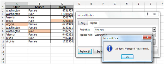
Replace by using the key “CTRL + H”
- In workbook press key “CTRL + H” ,“FIND and REPLACE” dialog box will appear.
- In which you have to define “FIND WHAT” and “REPLACE WITH”.

- Let’s say you want to replace to “New York” with “Washington”
- So write the “New York” in “Find what” box and “Washington” in “Replace with” box. Click on “Replace All”.
- You will get a message box which will inform you how many words you made replaced.
- Click on ok of message box.
- Close the Find and Replace dialog box.
This way you can find and replace in Microsoft Excel by the using the key Ctrl+F to find and Ctrl+H to replace text, numbers etc.
How do I search for a word or phrase across multiple sheets in a workbook in Excel 2007, 2010, 2013 and 2016?
Why would I want to search a whole workbook?
We think of Excel as being used primarily for numbers (although you might want to search for those, too), but I often encounter spreadsheets full of text. For example, when I’m localising text from US to UK English, or editing text that’s been translated, and it’s been output from a translation tool such as Trados, it often comes to me in an Excel spreadsheet.
Just like when I’m editing a Word or PDF file, I often want to either look for all instances of a word I want to change or check that I haven’t missed anything. And if that word might be in any one of many sheets in a workbook, I will want to search all of those sheets.
How do I perform a search in all the sheets of a workbook?
In this example, I want to find all the instances of the word “authorized” in all the many sheets in an Excel workbook.
First of all, press Control and F at the same time to bring up the Find and Replace dialogue box:

Using this search without changing anything will just search in the sheet I’m currently in.
Click on Options:

This brings up a load of options, including some other exciting ones we’re not looking at here, but which might be useful as well:

Click on the drop-down arrow to the right of Within: Sheet and change it to Workbook:

Now when you click “Find Next”, it will find the cell where that text is throughout the whole workbook.
In this article, we’ve learned how to search a whole workbook in Excel 2007, 2010, 2013 and 2016.
If you’ve found this article helpful, please do post a comment below, and if you think others would find it useful, please share it using the sharing buttons below the article. Thank you!
Other useful posts on Excel on this blog:
How to view two workbooks side by side in Excel 2007 and 2010
How to view two pages of a workbook at the same time
How do I print the column headings on every sheet in Excel?
How to print the column and row numbers/ letters and gridlines
How to change rows into columns and columns into rows in Excel
Freezing rows and columns in Excel – and freezing both at the same time
How to flip a column in Excel – turn it upside down but keep the exact same order!
I have written a macro which will search for a string in all the sheets of an Excel workbook. This macro will activate the first sheet as well as the cell in the sheet which contains the search string. If not found, then it will show a message.
I want to extend this functionality to cover all the sheets which contain this string and not just the first one. So I modified the macro, but it is not working as expected. I have given the code below and also commented at the place where it is showing the error.
Dim sheetCount As Integer
Dim datatoFind

Sub Button1_Click()

Find_Data

End Sub

Private Sub Find_Data()
    Dim counter As Integer
    Dim currentSheet As Integer
    Dim notFound As Boolean
    Dim yesNo As String

    notFound = True

    On Error Resume Next
    currentSheet = ActiveSheet.Index
    datatoFind = InputBox("Please enter the value to search for")
    If datatoFind = "" Then Exit Sub
    sheetCount = ActiveWorkbook.Sheets.Count
    If IsError(CDbl(datatoFind)) = False Then datatoFind = CDbl(datatoFind)
    For counter = 1 To sheetCount
        Sheets(counter).Activate

        Cells.Find(What:=datatoFind, After:=ActiveCell, LookIn:=xlFormulas, LookAt _
        :=xlPart, SearchOrder:=xlByRows, SearchDirection:=xlNext, MatchCase:= _
        False, SearchFormat:=False).Activate

        If InStr(1, ActiveCell.Value, datatoFind) Then
            If HasMoreValues(counter + 1) Then 'Not completing the method and directly entering
                yesNo = MsgBox("Do you want to continue search?", vbYesNo)
                If yesNo = vbNo Then
                    notFound = False
                    Exit For
                End If
            End If
            Sheets(counter).Activate
        End If
    Next counter
    If notFound Then
        MsgBox ("Value not found")
        Sheets(currentSheet).Activate
    End If
End Sub

Private Function HasMoreValues(ByVal sheetCounter As Integer) As Boolean
    HasMoreValues = False
    Dim str As String

    For counter = sheetCounter To sheetCount
        Sheets(counter).Activate

        str = Cells.Find(What:=datatoFind, After:=ActiveCell, LookIn:=xlFormulas, LookAt _
        :=xlPart, SearchOrder:=xlByRows, SearchDirection:=xlNext, MatchCase:= _
        False, SearchFormat:=False).Value 'Not going further than this i.e. following code is not executed

        If InStr(1, str, datatoFind) Then
            HasMoreValues = True
            Exit For
        End If
    Next counter
End Function
After searching online, I found there was no one universal solution for the problem of searching multiple excel spreadsheets online, so I decided to write my own excel spreadsheet that searches other excel spreadsheets, that can be found here.
Please note it’s only been tested in Excel 2010, but it should work in 2007 and earlier versions. If not, feel free to modify the code how you see fit.
The spreadsheet makes use of a custom userform and makes use of VBA code (which you’re welcome to use for any purpose). Naturally, macros etc have to be enabled for this to work, and the form appears upon opening the spreadsheet (you can access the code by pressing Alt + F11, going to the userform, and double-clicking the ‘Begin Search’ button in the design window).
Full explanation of functions and features can be found on the Github readme, but it basically allows you to specify two text search terms to search for within a specified directory (that you can navigate to), it can search said directory recursively, and open spreadsheets that are password protected (so long as you provide the password).
It will search individual sheets in each workbook on a cell level search. Depending on workbook size, it can take roughly a second to scan each workbook.
It displays all search results in a side window, including any spreadsheets it failed to open. These results can be saved to a text file for later reference.
The userform should be relatively self-explanatory, however the readme for it on Github goes into great depth on how to use. Again, free to use, it’s open-source.