Find function for excel

Функция НАЙТИ (FIND) в Excel используется для поиска текстового значения внутри строчки с текстом и указать порядковый номер буквы с которого начинается искомое слово в найденной строке.

Что возвращает функция

Возвращает числовое значение, обозначающее стартовую позицию текстовой строчки внутри другой текстовой строчки.

Синтаксис

=FIND(find_text, within_text, [start_num]) — английская версия

=НАЙТИ(искомый_текст;просматриваемый_текст;[нач_позиция]) — русская версия

Аргументы функции

• find_text (искомый_текст) — текст или строка которую вы хотите найти в рамках другой строки;
• within_text (просматриваемый_текст) — текст, внутри которого вы хотите найти аргумент find_text (искомый_текст);
• [start_num] ([нач_позиция]) — число, отображающее позицию, с которой вы хотите начать поиск. Если аргумент не указать, то поиск начнется сначала.

Дополнительная информация

• Если стартовое число не указано, то функция начинает поиск искомого текста с начала строки;
• Функция НАЙТИ чувствительна к регистру. Если вы хотите сделать поиск без учета регистра, используйте функцию SEARCH в Excel;
• Функция не учитывает подстановочные знаки при поиске. Если вы хотите использовать подстановочные знаки для поиска, используйте функцию SEARCH в Excel;
• Функция каждый раз возвращает ошибку, когда не находит искомый текст в заданной строке.

Примеры использования функции НАЙТИ в Excel

Пример 1. Ищем слово в текстовой строке (с начала строки)

На примере выше мы ищем слово «Доброе» в словосочетании «Доброе Утро». По результатам поиска, функция выдает число «1», которое обозначает, что слово «Доброе» начинается с первой по очереди буквы в, заданной в качестве области поиска, текстовой строке.

Обратите внимание, что так как функция НАЙТИ в Excel чувствительна к регистру, вы не сможете найти слово «доброе» в словосочетании «Доброе утро», так как оно написано с маленькой буквы. Для того, чтобы осуществить поиска без учета регистра следует пользоваться функцией SEARCH.

Пример 2. Ищем слово в текстовой строке (с заданным порядковым номером старта поиска)

Третий аргумент функции НАЙТИ указывает позицию, с которой функция начинает поиск искомого значения. На примере выше функция возвращает число «1» когда мы начинаем поиск слова «Доброе» в словосочетании «Доброе утро» с начала текстовой строки. Но если мы зададим аргумент функции start_num (нач_позиция) со значением «2», то функция выдаст ошибку, так как начиная поиск со второй буквы текстовой строки, она не может ничего найти.

Если вы не укажете номер позиции, с которой функции следует начинать поиск искомого аргумента, то Excel по умолчанию начнет поиск с самого начала текстовой строки.

Пример 3. Поиск текстового значения внутри текстовой строки с дублированным искомым значением

На примере выше мы ищем слово «Доброе» в словосочетании «Доброе Доброе утро». Когда мы начинаем поиск слова «Доброе» с начала текстовой строки, то функция выдает число «1», так как первое слово «Доброе» начинается с первой буквы в словосочетании «Доброе Доброе утро».

Но, если мы укажем в качестве аргумента start_num (нач_позиция) число «2» и попросим функцию начать поиск со второй буквы в заданной текстовой строке, то функция выдаст число «6», так как Excel находит искомое слово «Доброе» начиная со второй буквы словосочетания «Доброе Доброе утро» только на 6 позиции.

Purpose 

Return value 

Usage notes 

=FIND("p","apple") // returns 2
=FIND("z","apple") // returns #VALUE!

=FIND("a","Apple") // returns #VALUE!
=FIND("A","Apple") // returns 1

=ISNUMBER(FIND("p","apple")) // returns TRUE
=ISNUMBER(FIND("z","apple")) // returns FALSE

=FIND("x","20 x 30 x 50") // returns 4

=FIND("x","20 x 30 x 50",5) // returns 9

=IF(ISNUMBER(FIND(substring,A1)), "Yes", "No")

The FIND function is a built-in Worksheet Function (WS) in Microsoft Excel, which you can use to locate a sub-string or a specific character’s position within a text string. It is categorized as a TEXT function in Excel.

If the FIND function fails to find the text, it will return a #VALUE error. Note that the Excel FIND function will perform a case-sensitive search.

Excel FIND function is commonly used by financial analysts for locating specific data or text occurrences in a cell.

Syntax of Excel FIND function

=FIND(find_text, within_text, [start_num])

Arguments:

'find_text' – The text/sub-string you want to locate.
'within_text' – This argument is the string within which you wish to perform the search. You can supply a cell reference or type in the string into the formula.
'start_num' – This is an optional argument wherein you specify the character from which your search must begin. If you omit this argument, the function will assume this parameter as 1, i.e., the search will begin from the 1st character of the 'within_text' string.

Things to Remember

• The FIND function in Excel is case-sensitive and does not allow the usage of wildcard characters. For locating case-insensitive matches, take a look at the SEARCH function.
• The FIND function will search the 'find_text' argument in 'within_text' and return the first character’s position.
• You may search for either a substring or a character with the 'find_text'argument. You may use cell references or text characters for both 'find_text' and 'within_text' The FIND function will return ‘1’ when the 'find_text' argument is an empty string «».
• The FIND function returns #VALUE! error when:
  • The FIND function cannot locate 'find_text'in 'within_text' or
  • The 'start_num' argument is negative, 0, or greater than the length of 'within_text'

Examples of FIND function in Excel

Example 1 – Finding a word’s position in a text string

In this example, when you search for «Dallas» and reference the cell A2, which has the text string «Dallas, USA» the function will return ‘1’. Here, 1 represents the position of the searched word’s starting point.

On account of the FIND function’s case-sensitivity, entering «dallas» as an argument will return #VALUE! error.

Example 2 – Search for a word in a text string

The 'start_num' argument lets you decide the starting position for performing the search in the text string. You will see that in the above example, the FIND function returns ‘1’ when we put 1 as the 'start_num'. Essentially, it searches for the text «Dallas» in «Dallas, USA».

When we change 'start_num' to ‘2’, it returns an error because it then searches for «Dallas» in «allas, USA».

Note that skipping the 'start_num' argument will result in the FIND function assuming ‘1’ as the starting position.

Example 3 – When the searched text occurs multiple times in a text string

Since the FIND function refers to the 'start_num' argument to see if you would like to define a starting position, it returns ‘1’ when you input 'start_num' as 1. This is because it finds «Dallas» at position ‘1’ in «Dallas, Dallas, USA».

When you input 'start_num' as 2, though, you will see that it returns ‘9’. What is happening here is that the FIND function tries to look for the word «Dallas» in «allas, Dallas, USA» since you are asking the function to start searching from the second position. Here, 9 is the starting position of the 2nd «Dallas» in «Dallas, Dallas, USA».

Example 4 – Look for a specific character’s Nth occurrence in a string.

Let’s now assume that you would like to know the position of the second «,» in the list that has the format «City, Country, Continent».

For this, we will need to nest two FIND functions one within another. The second FIND function will go in the first FIND function as a third argument ('start_num'), like so:

=FIND(",",A2,FIND(",",A2)+1)

With the third argument, you are instructing the first FIND function to start searching for «,» exactly after the first occurrence of a «,» in the string.

Pro tip: You can use the CHAR and SUBSTITUTE functions to do this more simply, with the following formula:

=FIND(CHAR(1), SUBSTITUTE(A5,",",CHAR(1),2)

Example 5 – Retrieving the first part of a text string separated by «,» (comma)

Let’s assume you want the list of just the name of cities, without the name of the country, i.e., the characters right before «,»).

To accomplish this, we will use the LEFT function and the FIND function together. The FIND function will give us the position of «,» and the LEFT function will allow us to retrieve the name of the cities.

In our example, the FIND function will return 10 when executed on «Amsterdam, Netherlands». From this, we will subtract 1 since we don’t want to include the «,» in our output.

Next, we embed a FIND function into the LEFT function and use FIND(",", A2,1)-1 as the second argument, like so:

=LEFT(A2,FIND(",",A2,1)-1)

Example 6 – Retrieving the second part of a text string separated by «,» (comma)

Let’s take example 5, and try to retrieve the second part of the string.

To accomplish this, we will use the MID function and the FIND function together. The FIND function will give us the position of «,» and the MID function will allow us to fetch the specific string portion that we need.

In our example, the FIND function will return 10 when executed on «Amsterdam, Netherlands». From this, we will add 1 since we don’t want to include the «,» in our output.

Next, we use a MID function and pass the FIND function to it FIND(",", A2,1)+1 as the second argument, like so:

=MID(A2,FIND(",",A2,1)+1,100)

FIND function vs. SEARCH function in Excel

Both Find and Search functions have a similar syntax and application. However, there are 2 differences between these functions. Let’s dive into what these differences are:

1. Acceptance of wildcard characters

Unlike with the FIND function, you may use wildcard characters in the SEARCH function’s 'find_text' argument.

To match one character – we will use a question mark ‘?’, and to match a series of characters – we will use an asterisk mark ‘*’.

Let’s work this out with an example:

We will use the syntax:

=SEARCH(",*EUROPE",A2)

Notice how the Excel SEARCH function returns the first character’s position if you input both «,» and the «continent name» regardless of how many characters exist between the text string referred to in the 'within_text'argument.

Pro tip: For finding a ‘?’ or ‘*’, just add a tilde (~) in front of the question mark or the asterisk.

2. FIND is case-sensitive, while SEARCH is case-insensitive

As I mentioned previously, case-sensitivity is another differentiating factor between the two functions.

In our example, when using the FIND function to search for ‘A’ it returns the position of the capital A in ‘USA’. However, searching for ‘A’ with the SEARCH function returns the position of the ‘a’ in ‘Dallas’ because it is case-insensitive.

Handling #VALUE! errors in the FIND function

To deal with #VALUE! errors, we can use the IFERROR function.

Let’s revisit our first example where we first encountered a #VALUE! error with FIND function on account of the FIND function’s case-sensitivity.

Here is the syntax we will use to fix this:

=IFERROR(FIND("dallas",A3,1), "Not Found!")

Using this syntax, we will «trap» the error and replace it with a standard string in the second argument of the IFERROR function, which in our case is «Not Found!». So, until the FIND function is able to return a matched string, the function will keep returning «Not Found».

Excel FIND Function (Example + Video)

When to use Excel FIND Function

Excel FIND function can be used when you want to locate a text string within another text string and find its position.

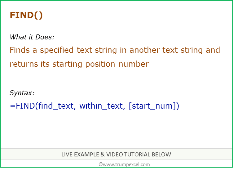
What it Returns

It returns a number that represents the starting position of the string you are finding in another string.

Syntax

=FIND(find_text, within_text, [start_num])

Input Arguments

• find_text – the text or string that you need to find.
• within_text – the text within which you want to find the find_text argument.
• [start_num] – a number that represents the position from which you want the search to begin. If you omit it, it starts from the beginning.

Additional Notes

• If the start number is not specified, then it starts looking from the beginning of the string.
• Excel FIND function is case-sensitive. If you want to do a case-insensitive search, use Excel SEARCH function.
• Excel FIND function cannot handle wildcard characters. If you want to use wildcard characters, use the Excel SEARCH function.
• It returns a #VALUE! error if the searched string is not found in the text.

Excel FIND Function – Examples

Here are four examples of using Excel FIND function:

Searching for a Word in a Text String (from the beginning)

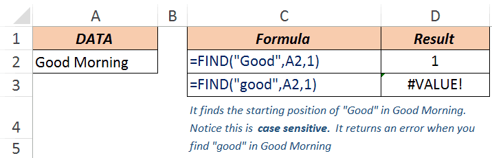
In the above example, when you look for the word Good in the text Good Morning, it returns 1, which is the position of the starting point of the searched word.

Note that Excel FIND function is case-sensitive. When you use good instead of Good, it returns a #VALUE! error.

If you are looking for a case-insensitive search, use Excel SEARCH function.

Finding a Word in a Text String (with a specified beginning)

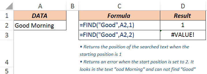
The third argument in the FIND function is the position within the text from where you want to start the search. In the example above, the function returns 1 when you search for the text Good in Good Morning and the starting position is 1.

However, it returns an error when you make it start at 2. Hence, it looks for the text Good in ood Morning. Since it can not find it, it returns an error.

Note: If you skip the last argument and don’t provide the starting position, by default it takes it as 1.

When there are Multiple Occurrence of the Searched Text

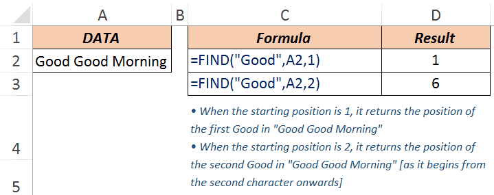
Excel FIND function starts looking in the specified text from the specified position. In the above example, when you look for the text Good in Good Good Morning with the starting position as 1, it returns 1, as it finds it at the beginning.

When you start the search from the second character onwards, it returns 6, as it finds the matching text at the sixth position.

Extracting Everything to the Left a Specified Character/String

Suppose you have the email ids do some superheroes as shown below and you want to extract only the username part (which would be the characters before the @).

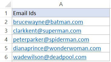
Below is the formula that will find the position of ‘@’ in each email id and extract all the characters to the left of it:

=LEFT(A2,FIND(“@”,A2,1)-1)

The FIND function in this formula gives the position of the ‘@’ character. The LEFT function that uses this position to extract the username.

For example, in the case of brucewayne@batman.com, the FIND function returns 11. LEFT function then uses FIND(“@”,A2,1)-1 as the second argument to get the username.

Note that 1 is subtracted from the value returned by the FIND function as we want to exclude the @ from the result of the LEFT function.

Excel FIND Function – VIDEO

Related Excel Functions:

• Excel LOWER Function.
• Excel UPPER Function.
• Excel PROPER Function.
• Excel REPLACE Function.
• Excel SEARCH Function.
• Excel SUBSTITUTE Function.

You May Also Like the Following Tutorials:

• How to Quickly Find and Remove Hyperlinks in Excel.
• How to Find Merged Cells in Excel.
• How to Find and Remove Duplicates in Excel.
• Using Find and Replace in Excel.

Поиск какого-либо значения в ячейках Excel довольно часто встречающаяся задача при программировании какого-либо макроса. Решить ее можно разными способами. Однако, в разных ситуациях использование того или иного способа может быть не оправданным. В данной статье я рассмотрю 2 наиболее распространенных способа.

Поиск перебором значений

Довольно простой в реализации способ. Например, найти в колонке «A» ячейку, содержащую «123» можно примерно так:

Sheets("Данные").Select
For y = 1 To Cells.SpecialCells(xlLastCell).Row
    If Cells(y, 1) = "123" Then
        Exit For
    End If
Next y
MsgBox "Нашел в строке: " + CStr(y)

Минусами этого так сказать «классического» способа являются: медленная работа и громоздкость. А плюсом является его гибкость, т.к. таким способом можно реализовать сколь угодно сложные варианты поиска с различными вычислениями и т.п.

Поиск функцией Find

Гораздо быстрее обычного перебора и при этом довольно гибкий. В простейшем случае, чтобы найти в колонке A ячейку, содержащую «123» достаточно такого кода:

Sheets("Данные").Select
Set fcell = Columns("A:A").Find("123")
If Not fcell Is Nothing Then
    MsgBox "Нашел в строке: " + CStr(fcell.Row)
End If

Вкратце опишу что делают строчки данного кода:
1-я строка: Выбираем в книге лист «Данные»;
2-я строка: Осуществляем поиск значения «123» в колонке «A», результат поиска будет в fcell;
3-я строка: Если удалось найти значение, то fcell будет содержать Range-объект, в противном случае — будет пустой, т.е. Nothing.

Полностью синтаксис оператора поиска выглядит так:

Find(What, After, LookIn, LookAt, SearchOrder, SearchDirection, MatchCase, MatchByte, SearchFormat)

What — Строка с текстом, который ищем или любой другой тип данных Excel

After — Ячейка, после которой начать поиск. Обратите внимание, что это должна быть именно единичная ячейка, а не диапазон. Поиск начинается после этой ячейки, а не с нее. Поиск в этой ячейке произойдет только когда весь диапазон будет просмотрен и поиск начнется с начала диапазона и до этой ячейки включительно.

LookIn — Тип искомых данных. Может принимать одно из значений: xlFormulas (формулы), xlValues (значения), или xlNotes (примечания).

LookAt — Одно из значений: xlWhole (полное совпадение) или xlPart (частичное совпадение).

SearchOrder — Одно из значений: xlByRows (просматривать по строкам) или xlByColumns (просматривать по столбцам)

SearchDirection — Одно из значений: xlNext (поиск вперед) или xlPrevious (поиск назад)

MatchCase — Одно из значений: True (поиск чувствительный к регистру) или False (поиск без учета регистра)

MatchByte — Применяется при использовании мультибайтных кодировок: True (найденный мультибайтный символ должен соответствовать только мультибайтному символу) или False (найденный мультибайтный символ может соответствовать однобайтному символу)

SearchFormat — Используется вместе с FindFormat. Сначала задается значение FindFormat (например, для поиска ячеек с курсивным шрифтом так: Application.FindFormat.Font.Italic = True), а потом при использовании метода Find указываем параметр SearchFormat = True. Если при поиске не нужно учитывать формат ячеек, то нужно указать SearchFormat = False.

Чтобы продолжить поиск, можно использовать FindNext (искать «далее») или FindPrevious (искать «назад»).

Примеры поиска функцией Find

Пример 1: Найти в диапазоне «A1:A50» все ячейки с текстом «asd» и поменять их все на «qwe»

With Worksheets(1).Range("A1:A50")
  Set c = .Find("asd", LookIn:=xlValues)
  Do While Not c Is Nothing
    c.Value = "qwe"
    Set c = .FindNext(c)
  Loop
End With

Обратите внимание: Когда поиск достигнет конца диапазона, функция продолжит искать с начала диапазона. Таким образом, если значение найденной ячейки не менять, то приведенный выше пример зациклится в бесконечном цикле. Поэтому, чтобы этого избежать (зацикливания), можно сделать следующим образом:

Пример 2: Правильный поиск значения с использованием FindNext, не приводящий к зацикливанию.

With Worksheets(1).Range("A1:A50")
  Set c = .Find("asd", lookin:=xlValues)
  If Not c Is Nothing Then
    firstResult = c.Address
    Do
      c.Font.Bold = True
      Set c = .FindNext(c)
      If c Is Nothing Then Exit Do
    Loop While c.Address <> firstResult
  End If
End With

В ниже следующем примере используется другой вариант продолжения поиска — с помощью той же функции Find с параметром After. Когда найдена очередная ячейка, следующий поиск будет осуществляться уже после нее. Однако, как и с FindNext, когда будет достигнут конец диапазона, Find продолжит поиск с его начала, поэтому, чтобы не произошло зацикливания, необходимо проверять совпадение с первым результатом поиска.

Пример 3: Продолжение поиска с использованием Find с параметром After.

With Worksheets(1).Range("A1:A50")
  Set c = .Find("asd", lookin:=xlValues)
  If Not c Is Nothing Then
    firstResult = c.Address
    Do
      c.Font.Bold = True
      Set c = .Find("asd", After:=c, lookin:=xlValues)
      If c Is Nothing Then Exit Do
    Loop While c.Address <> firstResult
  End If
End With

Следующий пример демонстрирует применение SearchFormat для поиска по формату ячейки. Для указания формата необходимо задать свойство FindFormat.

Пример 4: Найти все ячейки с шрифтом «курсив» и поменять их формат на обычный (не «курсив»)

lLastRow = Cells.SpecialCells(xlLastCell).Row
lLastCol = Cells.SpecialCells(xlLastCell).Column
Application.FindFormat.Font.Italic = True
With Worksheets(1).Range(Cells(1, 1), Cells(lLastRow, lLastCol))
  Set c = .Find("", SearchFormat:=True)
  Do While Not c Is Nothing
    c.Font.Italic = False
    Set c = .Find("", After:=c, SearchFormat:=True)
  Loop
End With

Примечание: В данном примере намеренно не используется FindNext для поиска следующей ячейки, т.к. он не учитывает формат (статья об этом: https://support.microsoft.com/ru-ru/kb/282151)

Коротко опишу алгоритм поиска Примера 4. Первые две строки определяют последнюю строку (lLastRow) на листе и последний столбец (lLastCol). 3-я строка задает формат поиска, в данном случае, будем искать ячейки с шрифтом Italic. 4-я строка определяет область ячеек с которой будет работать программа (с ячейки A1 и до последней строки и последнего столбца). 5-я строка осуществляет поиск с использованием SearchFormat. 6-я строка — цикл пока результат поиска не будет пустым. 7-я строка — меняем шрифт на обычный (не курсив), 8-я строка продолжаем поиск после найденной ячейки.

Хочу обратить внимание на то, что в этом примере я не стал использовать «защиту от зацикливания», как в Примерах 2 и 3, т.к. шрифт меняется и после «прохождения» по всем ячейкам, больше не останется ни одной ячейки с курсивом.

Свойство FindFormat можно задавать разными способами, например, так:

With Application.FindFormat.Font 
  .Name = "Arial" 
  .FontStyle = "Regular" 
  .Size = 10 
End With

Поиск последней заполненной ячейки с помощью Find

Следующий пример — применение функции Find для поиска последней ячейки с заполненными данными. Использованные в Примере 4 SpecialCells находит последнюю ячейку даже если она не содержит ничего, но отформатирована или в ней раньше были данные, но были удалены.

Пример 5: Найти последнюю колонку и столбец, заполненные данными

Set c = Worksheets(1).UsedRange.Find("*", SearchDirection:=xlPrevious)
If Not c Is Nothing Then
  lLastRow = c.Row: lLastCol = c.Column 
Else
  lLastRow = 1: lLastCol = 1
End If
MsgBox "lLastRow=" & lLastRow & " lLastCol=" & lLastCol

В этом примере используется UsedRange, который так же как и SpecialCells возвращает все используемые ячейки, в т.ч. и те, что были использованы ранее, а сейчас пустые. Функция Find ищет ячейку с любым значением с конца диапазона.

Поиск по шаблону (маске)

При поиске можно так же использовать шаблоны, чтобы найти текст по маске, следующий пример это демонстрирует.

Пример 6: Выделить красным шрифтом ячейки, в которых текст начинается со слова из 4-х букв, первая и последняя буквы «т», при этом после этого слова может следовать любой текст.

With Worksheets(1).Cells
  Set c = .Find("т??т*", LookIn:=xlValues, LookAt:=xlWhole)
  If Not c Is Nothing Then
    firstResult = c.Address
    Do
      c.Font.Color = RGB(255, 0, 0)
      Set c = .FindNext(c)
      If c Is Nothing Then Exit Do
    Loop While c.Address <> firstResult
  End If
End With

Для поиска функцией Find по маске (шаблону) можно применять символы:
* — для обозначения любого количества любых символов;
? — для обозначения одного любого символа;
~ — для обозначения символов *, ? и ~. (т.е. чтобы искать в тексте вопросительный знак, нужно написать ~?, чтобы искать именно звездочку (*), нужно написать ~* и наконец, чтобы найти в тексте тильду, необходимо написать ~~)

Поиск в скрытых строках и столбцах

Для поиска в скрытых ячейках нужно учитывать лишь один нюанс: поиск нужно осуществлять в формулах, а не в значениях, т.е. нужно использовать LookIn:=xlFormulas

Поиск даты с помощью Find

Если необходимо найти текущую дату или какую-то другую дату на листе Excel или в диапазоне с помощью Find, необходимо учитывать несколько нюансов:

• Тип данных Date в VBA представляется в виде #[месяц]/[день]/[год]#, соответственно, если необходимо найти фиксированную дату, например, 01 марта 2018 года, необходимо искать #3/1/2018#, а не «01.03.2018»
• В зависимости от формата ячеек, дата может выглядеть по-разному, поэтому, чтобы искать дату независимо от формата, поиск нужно делать не в значениях, а в формулах, т.е. использовать LookIn:=xlFormulas

Приведу несколько примеров поиска даты.

Пример 7: Найти текущую дату на листе независимо от формата отображения даты.

d = Date
Set c = Cells.Find(d, LookIn:=xlFormulas, LookAt:=xlWhole)
If Not c Is Nothing Then
  MsgBox "Нашел"
Else
  MsgBox "Не нашел"
End If

Пример 8: Найти 1 марта 2018 г.

d = #3/1/2018#
Set c = Cells.Find(d, LookIn:=xlFormulas, LookAt:=xlWhole)
If Not c Is Nothing Then
  MsgBox "Нашел"
Else
  MsgBox "Не нашел"
End If

Искать часть даты — сложнее. Например, чтобы найти все ячейки, где месяц «март», недостаточно искать «03» или «3». Не работает с датами так же и поиск по шаблону. Единственный вариант, который я нашел — это выбрать формат в котором месяц прописью для ячеек с датами и искать слово «март» в xlValues.

Тем не менее, можно найти, например, 1 марта независимо от года.

Пример 9: Найти 1 марта любого года.

d = #3/1/1900#
Set c = Cells.Find(Format(d, "m/d/"), LookIn:=xlFormulas, LookAt:=xlPart)
If Not c Is Nothing Then
  MsgBox "Нашел"
Else
  MsgBox "Не нашел"
End If

Sub Excel_FIND_Function()

End Sub

OBJECTS
Worksheets: The Worksheets object represents all of the worksheets in a workbook, excluding chart sheets.
Range: The Range object is a representation of a single cell or a range of cells in a worksheet.

PREREQUISITES
Worksheet Name: Have a worksheet named FIND.
String Range: Have the range of strings that you want to search within captured in range («B4:B7»).
Find sub-string: Have the sub-string that you want to search for in range («C5:C7»).
Start Position: In this example the start position only applies to the bottom two examples. Therefore, if using the exact same VBA code ensure that the start position value is captured in range («D6:D7»).

ADJUSTABLE PARAMETERS
Output Range: Select the output range by changing the cell references («E5»), («E6») and («E7») in the VBA code to any cell in the worksheet, that doesn’t conflict with formula.
String Range: Select the range of strings that you want to search within by changing the range («B5:B7») in the VBA code to any cell in the worksheet, that doesn’t conflict with formula.
Find sub-string: Select the sub-string that you want to search for by changing the cell references («C5»), («C6») and («C7») to any range in the worksheet, that doesn’t conflict with the formula.
Start Position: Select the start position value by changing the range («D6:D7») to any range in the worksheet, that doesn’t conflict with the formula.