Find from list excel - Word и Excel - помощь в работе с программами

Look up values in a list of data

Excel for Microsoft 365 Excel for the web Excel 2021 Excel 2019 Excel 2016 Excel 2013 Excel 2010 Excel 2007 More…Less

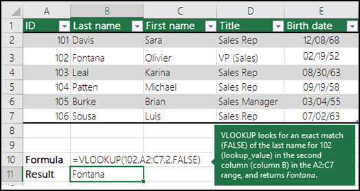
Let’s say that you want to look up an employee’s phone extension by using their badge number, or the correct rate of a commission for a sales amount. You look up data to quickly and efficiently find specific data in a list and to automatically verify that you are using correct data. After you look up the data, you can perform calculations or display results with the values returned. There are several ways to look up values in a list of data and to display the results.

What do you want to do?

Look up values vertically in a list by using an exact match
Look up values vertically in a list by using an approximate match
Look up values vertically in a list of unknown size by using an exact match
Look up values horizontally in a list by using an exact match
Look up values horizontally in a list by using an approximate match
Create a lookup formula with the Lookup Wizard (Excel 2007 only)

Look up values vertically in a list by using an exact match

To do this task, you can use the VLOOKUP function, or a combination of the INDEX and MATCH functions.

VLOOKUP examples

=VLOOKUP (B3,B2:E7,2,FALSE)

VLOOKUP looks for Fontana in the first column (column B) in the table_array B2:E7, and returns Olivier from the second column (column C) of the table_array. False returns an exact match.

For more information, see VLOOKUP function.

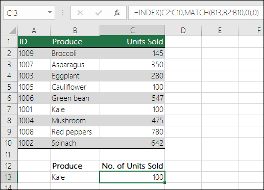
INDEX and MATCH examples

In simple English it means:

=INDEX(I want the return value from C2:C10, that will MATCH(Kale, which is somewhere in the B2:B10 array, where the return value is the first value corresponding to Kale))

The formula looks for the first value in C2:C10 that corresponds to Kale (in B7) and returns the value in C7 (100), which is the first value that matches Kale.

For more information, see INDEX function and MATCH function.

Top of Page

Look up values vertically in a list by using an approximate match

To do this, use the VLOOKUP function.

Important: Make sure the values in the first row have been sorted in an ascending order.

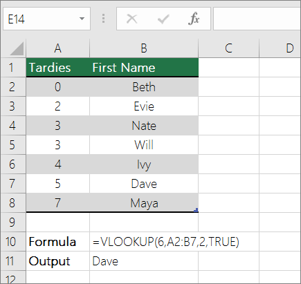
In the above example, VLOOKUP looks for the first name of the student who has 6 tardies in the A2:B7 range. There is no entry for 6 tardies in the table, so VLOOKUP looks for the next highest match lower than 6, and finds the value 5, associated to the first name Dave, and thus returns Dave.

For more information, see VLOOKUP function.

Top of Page

Look up values vertically in a list of unknown size by using an exact match

To do this task, use the OFFSET and MATCH functions.

Note: Use this approach when your data is in an external data range that you refresh each day. You know the price is in column B, but you don’t know how many rows of data the server will return, and the first column isn’t sorted alphabetically.

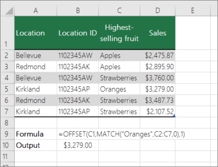
C1 is the upper left cells of the range (also called the starting cell).

MATCH(«Oranges»,C2:C7,0) looks for Oranges in the C2:C7 range. You should not include the starting cell in the range.

1 is the number of columns to the right of the starting cell where the return value should be from. In our example, the return value is from column D, Sales.

Top of Page

Look up values horizontally in a list by using an exact match

To do this task, use the HLOOKUP function. See an example below:

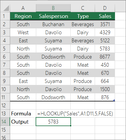
HLOOKUP looks up the Sales column, and returns the value from row 5 in the specified range.

For more information, see HLOOKUP function.

Top of Page

Look up values horizontally in a list by using an approximate match

To do this task, use the HLOOKUP function.

Important: Make sure the values in the first row have been sorted in an ascending order.

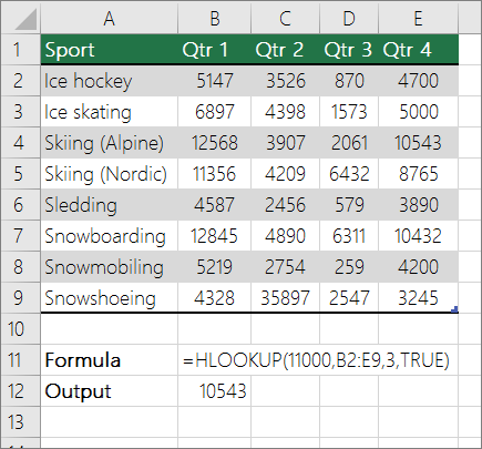
In the above example, HLOOKUP looks for the value 11000 in row 3 in the specified range. It does not find 11000 and hence looks for the next largest value less than 1100 and returns 10543.

For more information, see HLOOKUP function.

Top of Page

Create a lookup formula with the Lookup Wizard (Excel 2007 only)

Note: The Lookup Wizard add-in was discontinued in Excel 2010. This functionality has been replaced by the function wizard and the available Lookup and reference functions (reference).

In Excel 2007, the Lookup Wizard creates the lookup formula based on a worksheet data that has row and column labels. The Lookup Wizard helps you find other values in a row when you know the value in one column, and vice versa. The Lookup Wizard uses INDEX and MATCH in the formulas that it creates.

Click a cell in the range.
On the Formulas tab, in the Solutions group, click Lookup.
If the Lookup command is not available, then you need to load the Lookup Wizard add-in program.

How to load the Lookup Wizard Add-in program
Click the Microsoft Office Button , click Excel Options, and then click the Add-ins category.
In the Manage box, click Excel Add-ins, and then click Go.
In the Add-Ins available dialog box, select the check box next to Lookup Wizard, and then click OK.
Follow the instructions in the wizard.

Top of Page

Need more help?

Want more options?

Explore subscription benefits, browse training courses, learn how to secure your device, and more.

Communities help you ask and answer questions, give feedback, and hear from experts with rich knowledge.

Источник

Поиск какого-либо значения в ячейках Excel довольно часто встречающаяся задача при программировании какого-либо макроса. Решить ее можно разными способами. Однако, в разных ситуациях использование того или иного способа может быть не оправданным. В данной статье я рассмотрю 2 наиболее распространенных способа.

Поиск перебором значений

Довольно простой в реализации способ. Например, найти в колонке «A» ячейку, содержащую «123» можно примерно так:

Sheets("Данные").Select
For y = 1 To Cells.SpecialCells(xlLastCell).Row
    If Cells(y, 1) = "123" Then
        Exit For
    End If
Next y
MsgBox "Нашел в строке: " + CStr(y)

Минусами этого так сказать «классического» способа являются: медленная работа и громоздкость. А плюсом является его гибкость, т.к. таким способом можно реализовать сколь угодно сложные варианты поиска с различными вычислениями и т.п.

Поиск функцией Find

Гораздо быстрее обычного перебора и при этом довольно гибкий. В простейшем случае, чтобы найти в колонке A ячейку, содержащую «123» достаточно такого кода:

Sheets("Данные").Select
Set fcell = Columns("A:A").Find("123")
If Not fcell Is Nothing Then
    MsgBox "Нашел в строке: " + CStr(fcell.Row)
End If

Вкратце опишу что делают строчки данного кода:
1-я строка: Выбираем в книге лист «Данные»;
2-я строка: Осуществляем поиск значения «123» в колонке «A», результат поиска будет в fcell;
3-я строка: Если удалось найти значение, то fcell будет содержать Range-объект, в противном случае — будет пустой, т.е. Nothing.

Полностью синтаксис оператора поиска выглядит так:

Find(What, After, LookIn, LookAt, SearchOrder, SearchDirection, MatchCase, MatchByte, SearchFormat)

What — Строка с текстом, который ищем или любой другой тип данных Excel

After — Ячейка, после которой начать поиск. Обратите внимание, что это должна быть именно единичная ячейка, а не диапазон. Поиск начинается после этой ячейки, а не с нее. Поиск в этой ячейке произойдет только когда весь диапазон будет просмотрен и поиск начнется с начала диапазона и до этой ячейки включительно.

LookIn — Тип искомых данных. Может принимать одно из значений: xlFormulas (формулы), xlValues (значения), или xlNotes (примечания).

LookAt — Одно из значений: xlWhole (полное совпадение) или xlPart (частичное совпадение).

SearchOrder — Одно из значений: xlByRows (просматривать по строкам) или xlByColumns (просматривать по столбцам)

SearchDirection — Одно из значений: xlNext (поиск вперед) или xlPrevious (поиск назад)

MatchCase — Одно из значений: True (поиск чувствительный к регистру) или False (поиск без учета регистра)

MatchByte — Применяется при использовании мультибайтных кодировок: True (найденный мультибайтный символ должен соответствовать только мультибайтному символу) или False (найденный мультибайтный символ может соответствовать однобайтному символу)

SearchFormat — Используется вместе с FindFormat. Сначала задается значение FindFormat (например, для поиска ячеек с курсивным шрифтом так: Application.FindFormat.Font.Italic = True), а потом при использовании метода Find указываем параметр SearchFormat = True. Если при поиске не нужно учитывать формат ячеек, то нужно указать SearchFormat = False.

Чтобы продолжить поиск, можно использовать FindNext (искать «далее») или FindPrevious (искать «назад»).

Примеры поиска функцией Find

Пример 1: Найти в диапазоне «A1:A50» все ячейки с текстом «asd» и поменять их все на «qwe»

With Worksheets(1).Range("A1:A50")
  Set c = .Find("asd", LookIn:=xlValues)
  Do While Not c Is Nothing
    c.Value = "qwe"
    Set c = .FindNext(c)
  Loop
End With

Обратите внимание: Когда поиск достигнет конца диапазона, функция продолжит искать с начала диапазона. Таким образом, если значение найденной ячейки не менять, то приведенный выше пример зациклится в бесконечном цикле. Поэтому, чтобы этого избежать (зацикливания), можно сделать следующим образом:

Пример 2: Правильный поиск значения с использованием FindNext, не приводящий к зацикливанию.

With Worksheets(1).Range("A1:A50")
  Set c = .Find("asd", lookin:=xlValues)
  If Not c Is Nothing Then
    firstResult = c.Address
    Do
      c.Font.Bold = True
      Set c = .FindNext(c)
      If c Is Nothing Then Exit Do
    Loop While c.Address <> firstResult
  End If
End With

В ниже следующем примере используется другой вариант продолжения поиска — с помощью той же функции Find с параметром After. Когда найдена очередная ячейка, следующий поиск будет осуществляться уже после нее. Однако, как и с FindNext, когда будет достигнут конец диапазона, Find продолжит поиск с его начала, поэтому, чтобы не произошло зацикливания, необходимо проверять совпадение с первым результатом поиска.

Пример 3: Продолжение поиска с использованием Find с параметром After.

With Worksheets(1).Range("A1:A50")
  Set c = .Find("asd", lookin:=xlValues)
  If Not c Is Nothing Then
    firstResult = c.Address
    Do
      c.Font.Bold = True
      Set c = .Find("asd", After:=c, lookin:=xlValues)
      If c Is Nothing Then Exit Do
    Loop While c.Address <> firstResult
  End If
End With

Следующий пример демонстрирует применение SearchFormat для поиска по формату ячейки. Для указания формата необходимо задать свойство FindFormat.

Пример 4: Найти все ячейки с шрифтом «курсив» и поменять их формат на обычный (не «курсив»)

lLastRow = Cells.SpecialCells(xlLastCell).Row
lLastCol = Cells.SpecialCells(xlLastCell).Column
Application.FindFormat.Font.Italic = True
With Worksheets(1).Range(Cells(1, 1), Cells(lLastRow, lLastCol))
  Set c = .Find("", SearchFormat:=True)
  Do While Not c Is Nothing
    c.Font.Italic = False
    Set c = .Find("", After:=c, SearchFormat:=True)
  Loop
End With

Примечание: В данном примере намеренно не используется FindNext для поиска следующей ячейки, т.к. он не учитывает формат (статья об этом: https://support.microsoft.com/ru-ru/kb/282151)

Коротко опишу алгоритм поиска Примера 4. Первые две строки определяют последнюю строку (lLastRow) на листе и последний столбец (lLastCol). 3-я строка задает формат поиска, в данном случае, будем искать ячейки с шрифтом Italic. 4-я строка определяет область ячеек с которой будет работать программа (с ячейки A1 и до последней строки и последнего столбца). 5-я строка осуществляет поиск с использованием SearchFormat. 6-я строка — цикл пока результат поиска не будет пустым. 7-я строка — меняем шрифт на обычный (не курсив), 8-я строка продолжаем поиск после найденной ячейки.

Хочу обратить внимание на то, что в этом примере я не стал использовать «защиту от зацикливания», как в Примерах 2 и 3, т.к. шрифт меняется и после «прохождения» по всем ячейкам, больше не останется ни одной ячейки с курсивом.

Свойство FindFormat можно задавать разными способами, например, так:

With Application.FindFormat.Font 
  .Name = "Arial" 
  .FontStyle = "Regular" 
  .Size = 10 
End With

Поиск последней заполненной ячейки с помощью Find

Следующий пример — применение функции Find для поиска последней ячейки с заполненными данными. Использованные в Примере 4 SpecialCells находит последнюю ячейку даже если она не содержит ничего, но отформатирована или в ней раньше были данные, но были удалены.

Пример 5: Найти последнюю колонку и столбец, заполненные данными

Set c = Worksheets(1).UsedRange.Find("*", SearchDirection:=xlPrevious)
If Not c Is Nothing Then
  lLastRow = c.Row: lLastCol = c.Column 
Else
  lLastRow = 1: lLastCol = 1
End If
MsgBox "lLastRow=" & lLastRow & " lLastCol=" & lLastCol

В этом примере используется UsedRange, который так же как и SpecialCells возвращает все используемые ячейки, в т.ч. и те, что были использованы ранее, а сейчас пустые. Функция Find ищет ячейку с любым значением с конца диапазона.

Поиск по шаблону (маске)

При поиске можно так же использовать шаблоны, чтобы найти текст по маске, следующий пример это демонстрирует.

Пример 6: Выделить красным шрифтом ячейки, в которых текст начинается со слова из 4-х букв, первая и последняя буквы «т», при этом после этого слова может следовать любой текст.

With Worksheets(1).Cells
  Set c = .Find("т??т*", LookIn:=xlValues, LookAt:=xlWhole)
  If Not c Is Nothing Then
    firstResult = c.Address
    Do
      c.Font.Color = RGB(255, 0, 0)
      Set c = .FindNext(c)
      If c Is Nothing Then Exit Do
    Loop While c.Address <> firstResult
  End If
End With

Для поиска функцией Find по маске (шаблону) можно применять символы:
* — для обозначения любого количества любых символов;
? — для обозначения одного любого символа;
~ — для обозначения символов *, ? и ~. (т.е. чтобы искать в тексте вопросительный знак, нужно написать ~?, чтобы искать именно звездочку (*), нужно написать ~* и наконец, чтобы найти в тексте тильду, необходимо написать ~~)

Поиск в скрытых строках и столбцах

Для поиска в скрытых ячейках нужно учитывать лишь один нюанс: поиск нужно осуществлять в формулах, а не в значениях, т.е. нужно использовать LookIn:=xlFormulas

Поиск даты с помощью Find

Если необходимо найти текущую дату или какую-то другую дату на листе Excel или в диапазоне с помощью Find, необходимо учитывать несколько нюансов:

Тип данных Date в VBA представляется в виде #[месяц]/[день]/[год]#, соответственно, если необходимо найти фиксированную дату, например, 01 марта 2018 года, необходимо искать #3/1/2018#, а не «01.03.2018»
В зависимости от формата ячеек, дата может выглядеть по-разному, поэтому, чтобы искать дату независимо от формата, поиск нужно делать не в значениях, а в формулах, т.е. использовать LookIn:=xlFormulas

Приведу несколько примеров поиска даты.

Пример 7: Найти текущую дату на листе независимо от формата отображения даты.

d = Date
Set c = Cells.Find(d, LookIn:=xlFormulas, LookAt:=xlWhole)
If Not c Is Nothing Then
  MsgBox "Нашел"
Else
  MsgBox "Не нашел"
End If

Пример 8: Найти 1 марта 2018 г.

d = #3/1/2018#
Set c = Cells.Find(d, LookIn:=xlFormulas, LookAt:=xlWhole)
If Not c Is Nothing Then
  MsgBox "Нашел"
Else
  MsgBox "Не нашел"
End If

Искать часть даты — сложнее. Например, чтобы найти все ячейки, где месяц «март», недостаточно искать «03» или «3». Не работает с датами так же и поиск по шаблону. Единственный вариант, который я нашел — это выбрать формат в котором месяц прописью для ячеек с датами и искать слово «март» в xlValues.

Тем не менее, можно найти, например, 1 марта независимо от года.

Пример 9: Найти 1 марта любого года.

d = #3/1/1900#
Set c = Cells.Find(Format(d, "m/d/"), LookIn:=xlFormulas, LookAt:=xlPart)
If Not c Is Nothing Then
  MsgBox "Нашел"
Else
  MsgBox "Не нашел"
End If

Источник

A while back Vernon asked me how he could search one cell and compare it to a list of words. If any of the words in the list existed then return the matching word.

Ugh, I’ve written that 3 times and I’m not sure it’s any clearer…let’s look at an example.

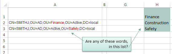
I’ve highlighted the matching words in column A red.

What we want Excel to do is to check the text string in column A to see if any of the words in our list in H1:H3 are present, if they are then return the matching word. Note: I’ve given cells H1:H3 the named range ‘list’.

There are a few ways we can tackle this so let’s take a look at our options.

Warning: this is quite an advanced topic which requires an array formula to solve it.

Update: It’s easier and more robust to use Power Query to search for text strings, including case and non-case sensitive searches.

Non-Case Sensitive Matching

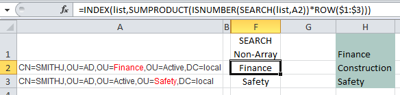
If you aren’t worried about case sensitive matches then you can use the SEARCH function with INDEX, SUMPRODUCT and ISNUMBER like this:

=INDEX(list,SUMPRODUCT(ISNUMBER(SEARCH(list,A2))*ROW($1:$3)))

In English our formula reads:

SEARCH cell A2 to see if it contains any words listed in cells H1:H3 (i.e. the named range ‘list’) and return the number of the character in cell A2 where the word starts. Our formula becomes:

=INDEX(list,SUMPRODUCT(ISNUMBER({20;#VALUE!;#VALUE!})*ROW($1:$3)))

i.e. in cell A2 the ‘F’ in the word ‘Finance’ starts in position 20.

Now using ISNUMBER test to see if the SEARCH formula returns any numbers (if it does it means there is a match). ISNUMBER will return TRUE if there is a number and FALSE if not (this gives us a list of Boolean TRUE or FALSE values). Our formula becomes:

=INDEX(list,SUMPRODUCT({TRUE;FALSE;FALSE}*ROW($1:$3)))

Use the ROW function to return an array of numbers {1;2;3} (see notes below on why I’ve used ROW in this formula). Our formula becomes:

=INDEX(list,SUMPRODUCT({TRUE;FALSE;FALSE}*{1;2;3}))

When you multiply Boolean TRUE/FALSE values they become their numeric equivalents i.e. TRUE = 1 and FALSE = 0. So our formula evaluates this ({TRUE;FALSE;FALSE}*{1;2;3}) like so: {1*1, 0*2, 0*3} and our formula becomes:

=INDEX(list,SUMPRODUCT({1;0;0}))

SUMPRODUCT simply sums the values {1+0+0} which gives us 1. Note: by using SUMPRODUCT we are avoiding the need for an array formula that requires CTRL+SHIFT+ENTER. Our formula becomes:

=INDEX(list,1)

Index can now go ahead and return the 1^st value in the range of cells H1:H3 which is ‘Finance’.

Note: the above formula will not work if a match isn’t found. If you want to return an error if a match isn’t found then you can use this variation:

=INDEX(list,IF(SUMPRODUCT(--ISNUMBER(SEARCH(list,A2)))<>0,SUMPRODUCT(ISNUMBER(SEARCH(list,A2))*ROW($1:$3)),NA()))

Not as elegant, is it? In which case you might prefer one of the array formulas below.

Notes about the ROW Function:

The ROW function simply returns the row number of a reference. e.g. ROW(A2) would return 2. When used in an array formula it will return an array of numbers. e.g. ROW(A2:A4) will return {2;3;4}. We can also give just the row reference(s) to the ROW function like so ROW(2:4).

In this formula we have used ROW to simply return an array of values {1;2;3} that represent the items in our ‘list’ i.e. Finance is 1, Construction is 2 and Safety is 3. Alternatively we could have typed {1;2;3} direct in our formula, or even referenced the named range like this ROW(list).

So you see using the ROW function is just a quick and clever way to generate an array of numbers.

What you must bear in mind when using the ROW function for this purpose is that we need a list of numbers from 1 to 3 because there are 3 words in our list and we’re trying to find the position of the matching word.

In this example the formula; ROW(list) will also work because our list happens to start on row 1 but if we were to start ‘list’ on row 2 we would come unstuck because ROW(list) would return {2;3;4} i.e. ‘list’ would actually reference cells H2:H4.

So, don’t get confused into thinking the ROW part of the formula is simply referencing the list or range of cells where the list is, the important point is that the ROW formula returns an array of numbers and we’re using those numbers to represent the number of rows in the ‘list’ which must always start with 1.

Functions Used

INDEX

SEARCH or FIND

ISNUMBER

SUMPRODUCT

ROW — Explained above.

Case Sensitive Matching

[updated Dec 5, 2013]

If your search is case sensitive then you not only need to replace SEARCH with FIND, but you also need to introduce an IF formula like so:

=INDEX(list,IF(SUMPRODUCT(ISNUMBER(FIND(list,A2))*ROW($1:$3))<>0,SUMPRODUCT(ISNUMBER(FIND(list,A2))*ROW($1:$3)),NA()))

Unfortunately it’s not as simple or elegant as the first non-case sensitive search. Instead the array formulas below are nicer

Array Formula Options

Below are some array formula options to achieve the same result. They use LARGE instead of SUMPRODUCT, and as a result you need to enter these by pressing CTRL+SHIFT+ENTER.

Non-case Sensitive:

[updated Dec 5, 2013]

=INDEX(list,LARGE(IF(ISNUMBER(SEARCH(list,A2)),ROW($1:$3)),1)) Press CTRL+SHIFT+ENTER

Case sensitive:

[updated Dec 5, 2013]

=INDEX(list,LARGE(IF(ISNUMBER(FIND(list,A2)),ROW($1:$3)),1)) Press CTRL+SHIFT+ENTER

Download

Enter your email address below to download the sample workbook.

By submitting your email address you agree that we can email you our Excel newsletter.

Thanks

Special thanks to Roberto for suggesting the ‘updated’ formulas above.

Источник

This will return the matching word or an error if no match is found. For this example I used the following.

List of words to search for: G1:G7
Cell to search in: A1

=INDEX(G1:G7,MAX(IF(ISERROR(FIND(G1:G7,A1)),-1,1)*(ROW(G1:G7)-ROW(G1)+1)))

Enter as an array formula by pressing Ctrl+Shift+Enter.

This formula works by first looking through the list of words to find matches, then recording the position of the word in the list as a positive value if it is found or as a negative value if it is not found. The largest value from this array is the position of the found word in the list. If no word is found, a negative value is passed into the INDEX() function, throwing an error.

To return the row number of a matching word, you can use the following:

=MAX(IF(ISERROR(FIND(G1:G7,A1)),-1,1)*ROW(G1:G7))

This also must be entered as an array formula by pressing Ctrl+Shift+Enter. It will return -1 if no match is found.

Источник

Содержание

1 Поисковая функция в Excel
- 1.1 Способ 1: простой поиск
- 1.2 Способ 2: поиск по указанному интервалу ячеек
- 1.3 Способ 3: Расширенный поиск
- 1.4 Помогла ли вам эта статья?
- 1.5 Поиск по нескольким листам с помощью макроса VBA
2 Простой поиск
3 Расширенный поиск
4 Разновидности поиска
- 4.1 Поиск совпадений
- 4.2 Фильтрация
- 4.3 Видео: Поиск в таблице Excel

В документах Microsoft Excel, которые состоят из большого количества полей, часто требуется найти определенные данные, наименование строки, и т.д. Очень неудобно, когда приходится просматривать огромное количество строк, чтобы найти нужное слово или выражение. Сэкономить время и нервы поможет встроенный поиск Microsoft Excel. Давайте разберемся, как он работает, и как им пользоваться.

Поисковая функция в программе Microsoft Excel предлагает возможность найти нужные текстовые или числовые значения через окно «Найти и заменить». Кроме того, в приложении имеется возможность расширенного поиска данных.

Способ 1: простой поиск

Простой поиск данных в программе Excel позволяет найти все ячейки, в которых содержится введенный в поисковое окно набор символов (буквы, цифры, слова, и т.д.) без учета регистра.

Находясь во вкладке «Главная», кликаем по кнопке «Найти и выделить», которая расположена на ленте в блоке инструментов «Редактирование». В появившемся меню выбираем пункт «Найти…». Вместо этих действий можно просто набрать на клавиатуре сочетание клавиш Ctrl+F.
После того, как вы перешли по соответствующим пунктам на ленте, или нажали комбинацию «горячих клавиш», откроется окно «Найти и заменить» во вкладке «Найти». Она нам и нужна. В поле «Найти» вводим слово, символы, или выражения, по которым собираемся производить поиск. Жмем на кнопку «Найти далее», или на кнопку «Найти всё».
При нажатии на кнопку «Найти далее» мы перемещаемся к первой же ячейке, где содержатся введенные группы символов. Сама ячейка становится активной.
Поиск и выдача результатов производится построчно. Сначала обрабатываются все ячейки первой строки. Если данные отвечающие условию найдены не были, программа начинает искать во второй строке, и так далее, пока не отыщет удовлетворительный результат.

Поисковые символы не обязательно должны быть самостоятельными элементами. Так, если в качестве запроса будет задано выражение «прав», то в выдаче будут представлены все ячейки, которые содержат данный последовательный набор символов даже внутри слова. Например, релевантным запросу в этом случае будет считаться слово «Направо». Если вы зададите в поисковике цифру «1», то в ответ попадут ячейки, которые содержат, например, число «516».

Для того, чтобы перейти к следующему результату, опять нажмите кнопку «Найти далее».

Так можно продолжать до тех, пор, пока отображение результатов не начнется по новому кругу.
В случае, если при запуске поисковой процедуры вы нажмете на кнопку «Найти все», все результаты выдачи будут представлены в виде списка в нижней части поискового окна. В этом списке находятся информация о содержимом ячеек с данными, удовлетворяющими запросу поиска, указан их адрес расположения, а также лист и книга, к которым они относятся. Для того, чтобы перейти к любому из результатов выдачи, достаточно просто кликнуть по нему левой кнопкой мыши. После этого курсор перейдет на ту ячейку Excel, по записи которой пользователь сделал щелчок.

Способ 2: поиск по указанному интервалу ячеек

Если у вас довольно масштабная таблица, то в таком случае не всегда удобно производить поиск по всему листу, ведь в поисковой выдаче может оказаться огромное количество результатов, которые в конкретном случае не нужны. Существует способ ограничить поисковое пространство только определенным диапазоном ячеек.

Выделяем область ячеек, в которой хотим произвести поиск.
Набираем на клавиатуре комбинацию клавиш Ctrl+F, после чего запуститься знакомое нам уже окно «Найти и заменить». Дальнейшие действия точно такие же, что и при предыдущем способе. Единственное отличие будет состоять в том, что поиск выполняется только в указанном интервале ячеек.

Способ 3: Расширенный поиск

Как уже говорилось выше, при обычном поиске в результаты выдачи попадают абсолютно все ячейки, содержащие последовательный набор поисковых символов в любом виде не зависимо от регистра.

К тому же, в выдачу может попасть не только содержимое конкретной ячейки, но и адрес элемента, на который она ссылается. Например, в ячейке E2 содержится формула, которая представляет собой сумму ячеек A4 и C3. Эта сумма равна 10, и именно это число отображается в ячейке E2. Но, если мы зададим в поиске цифру «4», то среди результатов выдачи будет все та же ячейка E2. Как такое могло получиться? Просто в ячейке E2 в качестве формулы содержится адрес на ячейку A4, который как раз включает в себя искомую цифру 4.

Но, как отсечь такие, и другие заведомо неприемлемые результаты выдачи поиска? Именно для этих целей существует расширенный поиск Excel.

После открытия окна «Найти и заменить» любым вышеописанным способом, жмем на кнопку «Параметры».
В окне появляется целый ряд дополнительных инструментов для управления поиском. По умолчанию все эти инструменты находятся в состоянии, как при обычном поиске, но при необходимости можно выполнить корректировку.

По умолчанию, функции «Учитывать регистр» и «Ячейки целиком» отключены, но, если мы поставим галочки около соответствующих пунктов, то в таком случае, при формировании результата будет учитываться введенный регистр, и точное совпадение. Если вы введете слово с маленькой буквы, то в поисковую выдачу, ячейки содержащие написание этого слова с большой буквы, как это было бы по умолчанию, уже не попадут. Кроме того, если включена функция «Ячейки целиком», то в выдачу будут добавляться только элементы, содержащие точное наименование. Например, если вы зададите поисковый запрос «Николаев», то ячейки, содержащие текст «Николаев А. Д.», в выдачу уже добавлены не будут.

По умолчанию, поиск производится только на активном листе Excel. Но, если параметр «Искать» вы переведете в позицию «В книге», то поиск будет производиться по всем листам открытого файла.

В параметре «Просматривать» можно изменить направление поиска. По умолчанию, как уже говорилось выше, поиск ведется по порядку построчно. Переставив переключатель в позицию «По столбцам», можно задать порядок формирования результатов выдачи, начиная с первого столбца.

В графе «Область поиска» определяется, среди каких конкретно элементов производится поиск. По умолчанию, это формулы, то есть те данные, которые при клике по ячейке отображаются в строке формул. Это может быть слово, число или ссылка на ячейку. При этом, программа, выполняя поиск, видит только ссылку, а не результат. Об этом эффекте велась речь выше. Для того, чтобы производить поиск именно по результатам, по тем данным, которые отображаются в ячейке, а не в строке формул, нужно переставить переключатель из позиции «Формулы» в позицию «Значения». Кроме того, существует возможность поиска по примечаниям. В этом случае, переключатель переставляем в позицию «Примечания».

Ещё более точно поиск можно задать, нажав на кнопку «Формат».

При этом открывается окно формата ячеек. Тут можно установить формат ячеек, которые будут участвовать в поиске. Можно устанавливать ограничения по числовому формату, по выравниванию, шрифту, границе, заливке и защите, по одному из этих параметров, или комбинируя их вместе.

Если вы хотите использовать формат какой-то конкретной ячейки, то в нижней части окна нажмите на кнопку «Использовать формат этой ячейки…».

После этого, появляется инструмент в виде пипетки. С помощью него можно выделить ту ячейку, формат которой вы собираетесь использовать.

После того, как формат поиска настроен, жмем на кнопку «OK».

Бывают случаи, когда нужно произвести поиск не по конкретному словосочетанию, а найти ячейки, в которых находятся поисковые слова в любом порядке, даже, если их разделяют другие слова и символы. Тогда данные слова нужно выделить с обеих сторон знаком «*». Теперь в поисковой выдаче будут отображены все ячейки, в которых находятся данные слова в любом порядке.
Как только настройки поиска установлены, следует нажать на кнопку «Найти всё» или «Найти далее», чтобы перейти к поисковой выдаче.

Как видим, программа Excel представляет собой довольно простой, но вместе с тем очень функциональный набор инструментов поиска. Для того, чтобы произвести простейший писк, достаточно вызвать поисковое окно, ввести в него запрос, и нажать на кнопку. Но, в то же время, существует возможность настройки индивидуального поиска с большим количеством различных параметров и дополнительных настроек.

Мы рады, что смогли помочь Вам в решении проблемы.

Задайте свой вопрос в комментариях, подробно расписав суть проблемы. Наши специалисты постараются ответить максимально быстро.

Помогла ли вам эта статья?

Да Нет

Добрый день!

Сегодня я хочу расширить границы использования функции ВПР и научить вас использовать эту функцию, что бы произвести поиск значений в Excel по нескольким листам вашего рабочего файла.

Как вы знаете или еще не знаете, я напоминаю, в чистом виде функция ВПР производит поиск только в одной таблице, а о том, что бы чистыми возможностями функции произвести поиск необходимого значения в нескольких листиках, это невозможно. Но, тем не менее, при большой необходимости можно схитрить и произвести поиск по двум листам. Для этого используем возможности логической функции ЕСЛИ и формула поиска будет выглядеть приблизительно так:

=ВПР (C3 ;ЕСЛИ (ЕНД (ВПР (C3 ;Таблица2!C3:D7 ;2; 0)); Таблица3! C3:D7 ;Таблица2! C3:D7 );2; 0).

Но такой вариант работает только с 2 таблицами, а в случае, когда листов больше, нужно увеличивать количество вложений для функции ЕСЛИ. Но при этом:

во-первых, если много листов, то есть огромный шанс что длина формулы будет больше допустимого размера и перестанет работать;
во-вторых, это просто непрактично, так как при работе такой мега-формулы возникает значительно риск ошибок и при изменениях придётся переделывать формулу.

Но, как всегда, выход есть. Рассмотрим небольшую хитрость с помощью, которой и будем искать в нужных листах. Начнем работу с создания перечня листов нашей книги, где будем производить поиск значений. В нашем случае это диапазон $E$3:$E$7. Теперь для получения значения в столбик «Найденная стоимость» согласно условию в столбике «Номенклатуру которую ищем» нам нужна формула:

{=ВПР (A3; ДВССЫЛ («’»&ИНДЕКС ($E$3:$E$7; ПОИСКПОЗ (ИСТИНА; СЧЁТЕСЛИ (ДВССЫЛ («’»&$E$3:$E$7 &»‘!C1:C50″) ;A3)> 0;0)) &»‘!C:D» );2;0)}

Как видите, формула выделена фигурными скобками, это означает, что её необходимо вводить как формулу массива с помощью горячего сочетания клавиш Ctrl+Shift+Enter. Это самое главное условие правильной работы этой формулы в других случаях она не будет работать. Формула объемная и требует объяснения принципа её работы. Функция ДВССЫЛ необходима, что бы конвертировать текстовые отображения ссылок на листы нашей книги в действительные. Сам принцип работы функции ДВССЫЛ, я описывать не буду, рассмотрим только необходимую формулу для этапа нашего вычисления: СЧЁТЕСЛИ (ДВССЫЛ («’»&$E$3:$E$7 &»‘! C1:C50″); A3).

Как следствие, при вычислении этого блока у нас формируется массив из некоторого количества значений, которые мы ищем, и которые повторяются на листах нашего списка, и имеет вид: СЧЁТЕСЛИ({2;0;0;0};A3). О работе функции СЧЁТЕСЛИ я писал отдельно и более подробно.

Следующим рассматриваемым блоком нашей композиции будет формула: ПОИСКПОЗ (ИСТИНА; СЧЁТЕСЛИ (ДВССЫЛ («’»&$E$3:$E$7 &»‘! C1:C50″); A3)>0;0), которая и работает с указанным выше блоком такого вида: ПОИСКПОЗ (ИСТИНА; СЧЁТЕСЛИ ({2;0;0;0}; A3)>0;0). Вследствие чего мы узнаем, какую позицию занимает имя листа в нашем массиве списке листов $E$3:$E$7. Теперь же при помощи функции ИНДЕКС мы получаем название листа, и можем применить его имя в структуре функции ДВССЫЛ, а она передаст полученное значение уже далее функции ВПР. Пошагово это будет выглядеть так:

=ВПР (A3; ДВССЫЛ («’»&ИНДЕКС ({«Таблица1″; « Таблица2»; « Таблица3»; «Таблица4»; «Таблица5»};1) &»‘! C:D»); 2;0);
=ВПР(A2;ДВССЫЛ(«’Таблица1′! C:D»);2;0);
=ВПР(A2;’Таблица1′!C:D;2;0).

Ну, вот мы и получили универсальную формулу, которая производит поиск значений в Excel и является очень гибкой и удобной. В случаях, когда возникнет необходимость добавить в рабочую книгу еще листы с таблицами, то необходимо всего на всего прописать их в списке рабочих листов $E$3:$E$7, изменив предварительно ее размер или попросту изначально сделать ее динамическим диапазоном, и править формулу будет не нужно.

Для большего удобства в столбике С, в графе «Где было найдено» можно прописать формулу которая будет наглядно показывать где была взята цифра, с какой таблицы вы получили значение, что значительно облегчает поисковую навигацию. Для получения названия таблицы необходима формула:

{=ИНДЕКС ($E$3:$E$7; ПОИСКПОЗ (ИСТИНА; СЧЁТЕСЛИ (ДВССЫЛ («’»&$E$3 :$E$7&»‘! C1:C50″); A3) >0;0))}

Поиск по нескольким листам с помощью макроса VBA

Для тех, кто хочет производить поиск значений в Excel по своей рабочей книге с помощью макросов или просто сделать рутинную операцию более автоматической предлагаю воспользоваться прописанной функцией пользователя, которая будет искать необходимое значение во всех, без исключения, даже в скрытых, листах рабочей книги, в которую вы ее пропишете. Макрос был найден на сайте excel — vba.ru, который любит такие фишки.

Функция будет иметь следующий вид:

Function VLookUpAllSheets(vCriteria As Variant, rTable As Range, lColNum As Long, Optional iPart As Integer = 1) As Variant

Dim rFndRng As Range

If iPart <> 1 Then iPart = 2

For i = 1 To Worksheets.Count

If Sheets(i).Name <> Application.Caller.Parent.Name Then

With Sheets(i)

Set rFndRng = .Range(rTable.Address).Resize(, 1).Find(vCriteria, , xlValues, iPart)

If Not rFndRng Is Nothing Then

VLookUpAllSheets = rFndRng.Offset(, lColNum — 1).Value

Exit For

End If

End With

End If

Next i

End Function

Расшифруются аргументы написанной функции так:

rTable – прописывается таблица, как в обыкновенной функции ВПР, для поиска значений;
vCriteria – аргумент, который указывает любое текстовое значение или ссылка на ячейку, которая содержит значение для поиска;
lColNum – прописывается тот номер столбика из аргумента rTable, значение в котором нам необходимо изъять, возможно, использовать ссылку на столбик с помощью функции СТОЛБЕЦ;
iPart – аргумент, в котором прописываем необходимый метод просмотра. Когда аргумент не указан или указан аргумент равно 1, в таком случае будет проводиться поиск с полным совпадением значений в ячейках. В таких случаях есть возможность применить символы подстановки: «*» и «?». Если же, в аргументе указано другое значение кроме 1, функция будет искать, и отбирать значения при частичном вхождении.

Я надеюсь, что поиск значений в Excel функцией ВПР по нескольким листам у вас получился, и вы могли быстро собрать нужные данные в ваших таблицах, а также научились создавать удобные и классные отчёты. Если у вас есть чем дополнить меня пишите комментарии, я буду их ждать с нетерпением, ставьте лайки и делитесь полезной статьей в соц.сетях!

Не забудьте подкинуть автору на кофе…

Основное назначение офисной программы Excel – осуществление расчётов. Документ этой программы (Книга) может содержать много листов с длинными таблицами, заполненными числами, текстом или формулами. Автоматизированный быстрый поиск позволяет найти в них необходимые ячейки.

Простой поиск

Чтобы произвести поиск значения в таблице Excel, необходимо на вкладке «Главная» открыть выпадающий список инструмента «Найти и заменить» и щёлкнуть пункт «Найти». Тот же эффект можно получить, используя сочетание клавиш Ctrl + F.

В простейшем случае в появившемся окне «Найти и заменить» надо ввести искомое значение и щёлкнуть «Найти всё».

Как видно, в нижней части диалогового окна появились результаты поиска. Найденные значения подчёркнуты красным в таблице. Если вместо «Найти все» щёлкнуть «Найти далее», то сначала будет произведён поиск первой ячейки с этим значением, а при повторном щелчке – второй.

Аналогично производится поиск текста. В этом случае в строке поиска набирается искомый текст.

Если данные или текст ищется не во всей экселевской таблице, то область поиска предварительно должна быть выделена.

Расширенный поиск

Предположим, что требуется найти все значения в диапазоне от 3000 до 3999. В этом случае в строке поиска следует набрать 3???. Подстановочный знак «?» заменяет собой любой другой.

Анализируя результаты произведённого поиска, можно отметить, что, наряду с правильными 9 результатами, программа также выдала неожиданные, подчёркнутые красным. Они связаны с наличием в ячейке или формуле цифры 3.

Можно удовольствоваться большинством полученных результатов, игнорируя неправильные. Но функция поиска в эксель 2010 способна работать гораздо точнее. Для этого предназначен инструмент «Параметры» в диалоговом окне.

Щёлкнув «Параметры», пользователь получает возможность осуществлять расширенный поиск. Прежде всего, обратим внимание на пункт «Область поиска», в котором по умолчанию выставлено значение «Формулы».

Это означает, что поиск производился, в том числе и в тех ячейках, где находится не значение, а формула. Наличие в них цифры 3 дало три неправильных результата. Если в качестве области поиска выбрать «Значения», то будет производиться только поиск данных и неправильные результаты, связанные с ячейками формул, исчезнут.

Для того чтобы избавиться от единственного оставшегося неправильного результата на первой строчке, в окне расширенного поиска нужно выбрать пункт «Ячейка целиком». После этого результат поиска становимся точным на 100%.

Такой результат можно было бы обеспечить, сразу выбрав пункт «Ячейка целиком» (даже оставив в «Области поиска» значение «Формулы»).

Теперь обратимся к пункту «Искать».

Если вместо установленного по умолчанию «На листе» выбрать значение «В книге», то нет необходимости находиться на листе искомых ячеек. На скриншоте видно, что пользователь инициировал поиск, находясь на пустом листе 2.

Следующий пункт окна расширенного поиска – «Просматривать», имеющий два значения. По умолчанию установлено «по строкам», что означает последовательность сканирования ячеек по строкам. Выбор другого значения – «по столбцам», поменяет только направление поиска и последовательность выдачи результатов.

При поиске в документах Microsoft Excel, можно использовать и другой подстановочный знак – «*». Если рассмотренный «?» означал любой символ, то «*» заменяет собой не один, а любое количество символов. Ниже представлен скриншот поиска по слову Louisiana.

Иногда при поиске необходимо учитывать регистр символов. Если слово louisiana будет написано с маленькой буквы, то результаты поиска не изменятся. Но если в окне расширенного поиска выбрать «Учитывать регистр», то поиск окажется безуспешным. Программа станет считать слова Louisiana и louisiana разными, и, естественно, не найдёт первое из них.

Разновидности поиска

Поиск совпадений

Иногда бывает необходимо обнаружить в таблице повторяющиеся значения. Чтобы произвести поиск совпадений, сначала нужно выделить диапазон поиска. Затем, на той же вкладке «Главная» в группе «Стили», открыть инструмент «Условное форматирование». Далее последовательно выбрать пункты «Правила выделения ячеек» и «Повторяющиеся значения».

Результат представлен на скриншоте ниже.

При необходимости пользователь может поменять цвет визуального отображения совпавших ячеек.

Фильтрация

Другая разновидность поиска – фильтрация. Предположим, что пользователь хочет в столбце B найти числовые значения в диапазоне от 3000 до 4000.

Выделить первый столбец с заголовком.
На той же вкладке «Главная» в разделе «Редактирование» открыть инструмент «Сортировка и фильтр», и щёлкнуть пункт «Фильтр».
В верхней строчке столбца B появляется треугольник – условный знак списка. После его открытия в списке «Числовые фильтры» щёлкнуть пункт «между».
В окне «Пользовательский автофильтр» следует ввести начальное и конечное значение плюс OK.

Как видно, отображаться стали только строки, удовлетворяющие введённому условию. Все остальные оказались временно скрытыми. Для возврата к начальному состоянию следует повторить шаг 2.

Различные варианты поиска были рассмотрены на примере Excel 2010. Как сделать поиск в эксель других версий? Разница в переходе к фильтрации есть в версии 2003. В меню «Данные» следует последовательно выбрать команды «Фильтр», «Автофильтр», «Условие» и «Пользовательский автофильтр».

Видео: Поиск в таблице Excel

Источник

Author: Oscar Cronquist Article last updated on February 01, 2023

This article demonstrates several ways to check if a cell contains any value based on a list. The first example shows how to check if any of the values in the list is in the cell.

The remaining examples show formulas that also return the matching values. You may need different formulas based on the Excel version you are using.

Read this article If cell equals value from list to match the entire cell to any value from a list. To match a single cell to a single value read this: If cell contains text

To check if a cell contains all values in the list read this: If cell contains multiple values

What’s on this page

Check if the cell contains any value in the list
Display matches if cell contains text from list (Excel 2019)
Display matches if cell contains text from list (Earlier Excel versions)
Filter delimited values not in list (Excel 365)

1. Check if the cell contains any value in the list

The image above shows an array formula in cell C3 that checks if cell B3 contains at least one of the values in List (E3:E7), it returns «Yes» if any of the values are found in column B and returns nothing if the cell contains none of the values.

For example, cell B3 contains XBF which is found in cell E7. Cell B4 contains text ZDS found in cell E6. Cell C5 contains no values in the list.

=IF(OR(COUNTIF(B3,»*»&$E$3:$E$7&»*»)), «Yes», «»)

You need to enter this formula as an array formula if you are not an Excel 365 subscriber. There is another formula below that doesn’t need to be entered as an array formula, however, it is slightly larger and more complicated.

Type formula in cell C3.
Press and hold CTRL + SHIFT simultaneously.
Press Enter once.
Release all keys.

Excel adds curly brackets to the formula automatically if you successfully entered the array formula. Don’t enter the curly brackets yourself.

1.1 Explaining formula in cell C3

Step 1 — Check if the cell contains any of the values in the list

The COUNTIF function lets you count cells based on a condition, however, it also allows you to count cells based on multiple conditions if you use a cell range instead of a cell.

COUNTIF(range, criteria)

The criteria argument utilizes a beginning and ending asterisk in order to match a text string and not the entire cell value, asterisks are one of two wildcard characters that you are allowed to use.

The ampersands concatenate the asterisks to cell range E3:E7.

COUNTIF(B3,»*»&$E$3:$E$7&»*»)

becomes

COUNTIF(«LNU, YNO, XBF», {«*MVN*»; «*QLL*»; «*BQX*»; «*ZDS*»; «*XBF*»})

and returns this array

{0; 0; 0; 0; 1}

which tells us that the last value in the list is found in cell B3.

Step 2 — Return TRUE if at least one value is 1

The OR function returns TRUE if at least one of the values in the array is TRUE, the numerical equivalent to TRUE is 1.

OR({0; 0; 0; 0; 1})

returns TRUE.

Step 3 — Return Yes or nothing

The IF function then returns «Yes» if the logical test evaluates to TRUE and nothing if the logical test returns FALSE.

IF(TRUE, «Yes», «»)

returns «Yes» in cell B3.

Regular formula

The following formula is quite similar to the formula above except that it is a regular formula and it has an additional INDEX function.

=IF(OR(INDEX(COUNTIF(B3,»*»&$E$3:$E$7&»*»),)), «Yes», «»)

2. Display matches if the cell contains text from a list

The image above demonstrates a formula that checks if a cell contains a value in the list and then returns that value. If multiple values match then all matching values in the list are displayed.

For example, cell B3 contains «ZDS, YNO, XBF» and cell range E3:E7 has two values that match, «ZDS» and «XBF».

Formula in cell C3:

=TEXTJOIN(«, «, TRUE, IF(COUNTIF(B3, «*»&$E$3:$E$7&»*»), $E$3:$E$7, «»))

The TEXTJOIN function is available for Office 2019 and Office 365 subscribers. You will get a #NAME error if your Excel version is missing this function. Office 2019 users may need to enter this formula as an array formula.

The next formula works with most Excel versions.

Array formula in cell C3:

=INDEX($E$3:$E$7, MATCH(1, COUNTIF(B3, «*»&$E$3:$E$7&»*»), 0))

However, it only returns the first match. There is another formula below that returns all matching values, check it out.

How to enter an array formula

2.1 Explaining formula in cell C3

Step 1 — Count cells containing text strings

The COUNTIF function lets you count cells based on a condition, we are going to use multiple conditions. I am going to use asterisks to make the COUNTIF function check for a partial match.

The asterisk is one of two wild card characters that you can use, it matches 0 (zero) to any number of any characters.

COUNTIF(B3, «*»&$E$3:$E$7&»*»)

becomes

COUNTIF(«ZDS, YNO, XBF», {«*MVN*»; «*QLL*»; «*BQX*»; «*ZDS*»; «*XBF*»})

and returns {1; 0; 0; 0; 1}.

This array contains as many values as there values in the list, the position of each value in the array matches the position of the value in the list. This means that we can tell from the array that the first value and the last value is found in cell B3.

Step 2 — Return the actual value

The IF function returns one value if the logical test is TRUE and another value if the logical test is FALSE.

IF(logical_test, [value_if_true], [value_if_false])

This allows us to create an array containing values that exists in cell B3.

IF(COUNTIF(B3, «*»&$E$3:$E$7&»*»), $E$3:$E$7, «»)

becomes

IF(COUNTIF(«ZDS, YNO, XBF», {«*MVN*»; «*QLL*»; «*BQX*»; «*ZDS*»; «*XBF*»}), {«*MVN*»; «*QLL*»; «*BQX*»; «*ZDS*»; «*XBF*»}, «»)

and returns {«»;»»;»»;»ZDS»;»XBF»}.

Step 3 — Concatenate values in array

The TEXTJOIN function allows you to combine text strings from multiple cell ranges and also use delimiting characters if you want.

TEXTJOIN(delimiter, ignore_empty, text1, [text2], …)

TEXTJOIN(«, «, TRUE, IF(COUNTIF(B3, «*»&$E$3:$E$7&»*»), $E$3:$E$7, «»))

becomes

TEXTJOIN(«, «, TRUE, {«»;»»;»»;»ZDS»;»XBF»})

and returns text strings ZDS, XBF.

3. Display matches if cell contains text from a list (Earlier Excel versions)

The image above demonstrates a formula that returns multiple matches if the cell contains values from a list. This array formula works with most Excel versions.

Array formula in cell C3:

=IFERROR(INDEX($G$3:$G$7, SMALL(IF(COUNTIF($B3, «*»&$G$3:$G$7&»*»), MATCH(ROW($G$3:$G$7), ROW($G$3:$G$7)), «»), COLUMNS($A$1:A1))), «»)

How to enter an array formula

Copy cell C3 and paste to cell range C3:E15.

3.1 Explaining formula in cell C3

Step 1 — Identify matching values in cell

The COUNTIF function lets you count cells based on a condition, we are going to use a cell range instead. This will return an array of values.

COUNTIF($B3, «*»&$G$3:$G$7&»*»)

becomes

COUNTIF(«ZDS, YNO, XBF», {«*MVN*»; «*QLL*»; «*BQX*»; «*ZDS*»; «*XBF*»})

and returns {0; 0; 0; 1; 1}.

Step 2 — Calculate relative positions of matching values

The IF function returns one value if the logical test is TRUE and another value if the logical test is FALSE.

IF(logical_test, [value_if_true], [value_if_false])

This allows us to create an array containing values representing row numbers.

IF(COUNTIF($B3, «*»&$G$3:$G$7&»*»), MATCH(ROW($G$3:$G$7), ROW($G$3:$G$7)), «»)

becomes

IF({0; 0; 0; 2; 1}, MATCH(ROW($G$3:$G$7), ROW($G$3:$G$7)), «»)

becomes

IF({0; 0; 0; 2; 1}, {1; 2; 3; 4; 5}, «»)

and returns {«»; «»; «»; 4; 5}.

Step 3 — Extract the k-th smallest number

I am going to use the SMALL function to be able to extract one value in each cell in the next step.

SMALL(array, k)

SMALL(IF(COUNTIF($B3, «*»&$G$3:$G$7&»*»), MATCH(ROW($G$3:$G$7), ROW($G$3:$G$7)), «»), COLUMNS($A$1:A1)))

becomes

SMALL({«»; «»; «»; 4; 5}, COLUMNS($A$1:A1)))

The COLUMNS function calculates the number of columns in a cell range, however, the cell reference in our formula grows when you copy the cell and paste to adjacent cells to the right.

SMALL({0; 0; 0; 4; 5}, COLUMNS($A$1:A1)))

becomes

SMALL({«»; «»; «»; 4; 5}, 1)

and returns 4.

Step 4 — Return value based on row number

The INDEX function returns a value from a cell range or array, you specify which value based on a row and column number. Both the [row_num] and [column_num] are optional.

INDEX(array, [row_num], [column_num])

INDEX($G$3:$G$7, SMALL(IF(COUNTIF($B3, «*»&$G$3:$G$7&»*»), MATCH(ROW($G$3:$G$7), ROW($G$3:$G$7)), «»), COLUMNS($A$1:A1)))

becomes

INDEX($G$3:$G$7, 4)

becomes

INDEX({«MVN»;»QLL»;»BQX»;»ZDS»;»XBF»}, 4)

and returns «ZDS» in cell C3.

Step 5 — Remove error values

The IFERROR function lets you catch most errors in Excel formulas except #SPILL! errors. Be careful when using the IFERROR function, it may make it much harder spotting formula errors.

IFERROR(value, value_if_error)

There are two arguments in the IFERROR function. The value argument is returned if it is not evaluating to an error. The value_if_error argument is returned if the value argument returns an error.

IFERROR(INDEX($G$3:$G$7, SMALL(IF(COUNTIF($B3, «*»&$G$3:$G$7&»*»), MATCH(ROW($G$3:$G$7), ROW($G$3:$G$7)), «»), COLUMNS($A$1:A1))), «»)

4. Filter delimited values not in the list (Excel 365)

The formula in cell C3 lists values in cell B3 that are not in the List specified in cell range E3:E7. The formula returns #CALC! error if all values are in the list, see cell C14 as an example.

Excel 365 dynamic array formula in cell C3:

=LET(z,TRIM(TEXTSPLIT(B3,,»,»)),TEXTJOIN(«, «,TRUE,FILTER(z,NOT(COUNTIF($E$3:$E$7,z)))))

4.1 Explaining formula

Step 1 — Split values with a delimiting character

The TEXTSPLIT function splits a string into an array based on delimiting values.

Function syntax: TEXTSPLIT(Input_Text, col_delimiter, [row_delimiter], [Ignore_Empty])

TEXTSPLIT(B3,,»,»)

becomes

TEXTSPLIT(«ZDS, VTO, XBF»,,»,»)

and returns

{«ZDS»; » VTO»; » XBF»}

Step 2 — Remove leading and trailing spaces

The TRIM function deletes all blanks or space characters except single blanks between words in a cell value.

Function syntax: TRIM(text)

TRIM(TEXTSPLIT(B3,,»,»))

becomes

TRIM({«ZDS»; » VTO»; » XBF»})

and returns

{«ZDS»; «VTO»; «XBF»}

Step 3 — Check if values are in list

The COUNTIF function calculates the number of cells that is equal to a condition.

Function syntax: COUNTIF(range, criteria)

COUNTIF($E$3:$E$7,TRIM(TEXTSPLIT(B3,,»,»)))

becomes

COUNTIF({«MVN»;»QLL»;»BQX»;»ZDS»;»XBF»},{«ZDS»; «VTO»; «XBF»})

and returns

{1; 0; 1}

These numbers indicate if a value is found in the list, zero means not in the list and 1 or higher means that the value is in the list at least once.

The number’s position corresponds to the position of the values. {1; 0; 1} — {«ZDS»; «VTO»; «XBF»} meaning «ZDS» and «XBF» are in the list and «VTO» not.

Step 4 — Not

The NOT function returns the boolean opposite to the given argument.

Function syntax: NOT(logical)

NOT(COUNTIF($E$3:$E$7,TRIM(TEXTSPLIT(B3,,»,»))))

becomes

NOT({1; 0; 1})

and returns

{FALSE; TRUE; FALSE}.

0 (zero) is equivalent to FALSE. The boolean opposite is TRUE.

Any other number than 0 (zero) is equivalent to TRUE. The boolean opposite is FALSE.

Step 5 — Filter

The FILTER function extracts values/rows based on a condition or criteria.

Function syntax: FILTER(array, include, [if_empty])

FILTER(TRIM(TEXTSPLIT(B3,,»,»)),NOT(COUNTIF($E$3:$E$7,TRIM(TEXTSPLIT(B3,,»,»)))))

becomes

FILTER({«ZDS»; «VTO»; «XBF»},{FALSE; TRUE; FALSE})

and returns

«VTO».

Step 6 — Join

The TEXTJOIN function combines text strings from multiple cell ranges.

Function syntax: TEXTJOIN(delimiter, ignore_empty, text1, [text2], …)

TEXTJOIN(«, «,TRUE,FILTER(TRIM(TEXTSPLIT(B3,,»,»)),NOT(COUNTIF($E$3:$E$7,TRIM(TEXTSPLIT(B3,,»,»))))))

becomes

TEXTJOIN(«, «,TRUE,{«VTO»})

and returns

«VTO».

Step 7 — Shorten the formula

The LET function lets you name intermediate calculation results which can shorten formulas considerably and improve performance.

Function syntax: LET(name1, name_value1, calculation_or_name2, [name_value2, calculation_or_name3…])

TEXTJOIN(«, «,TRUE,FILTER(TRIM(TEXTSPLIT(B3,,»,»)),NOT(COUNTIF($E$3:$E$7,TRIM(TEXTSPLIT(B3,,»,»))))))

z — TRIM(TEXTSPLIT(B3,,»,»))

LET(z,TRIM(TEXTSPLIT(B3,,»,»)),TEXTJOIN(«, «,TRUE,FILTER(z,NOT(COUNTIF($E$3:$E$7,z)))))

Источник

Searching a Microsoft Excel spreadsheet may seem easy. While Ctrl + F can help you find most things in a spreadsheet, you’ll want to use more sophisticated tools to find and extract data based on specific values. We’ll help you save tons of time with our list of advanced search functions.

Once you know how to search in Excel using lookup, it won’t matter how big your spreadsheets get, you’ll always be able to find what you need!

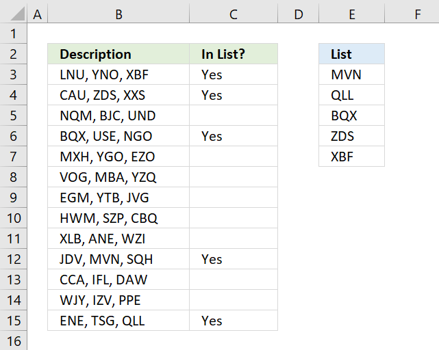
1. The VLOOKUP Function

The VLOOKUP function lets you find a specific value within a column and extract values from the corresponding row in adjoining columns. Two examples where you might do this are (1) looking up an employee’s last name by their employee number, or (2) finding a phone number by specifying the last name.

Here’s the syntax of the function:

 =VLOOKUP([lookup_value], [table_array], [col_index_num], [range_lookup])

[lookup_value] is the piece of information that you already have. For example, if you need to know what state a city is in, it would be the name of the city.
[table_array] lets you specify the cells in which the function will look for the lookup and return values. When selecting your range, be sure that the first column included in your array is the one that will include your lookup value!
[col_index_num] is the number of the column that contains the return value.
[range_lookup] is an optional argument, and takes 1 or 0, though you could also enter TRUE or FALSE. If you enter 1 or omit this argument, the function looks for an approximate value, but we’ve found this to be hit-or-miss. In the example below, a VLOOKUP looking for a score of 100 returns 90. Looking for a lower value, for example 88, returned an error.

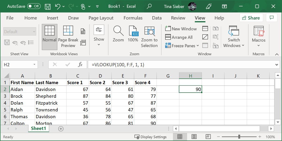
Let’s take a look at how you might use this. This spreadsheet contains student names and scores for four different tests. Let’s say you want to find score #4 for the student with the last name «Davidson.» VLOOKUP makes it easy.

Here’s the formula you’d use:

 =VLOOKUP("Davidson

Because the fourth score is the fifth column over from the last name we’re looking for, 5 is the column index argument. Note that when you’re looking for text, setting [range_lookup] to 0 is a good idea. Without it, you can get bad results.

Here’s the result:

It returned 79, which is score #4 of the student we queried.

Notes on VLOOKUP

A few things are good to remember when you’re using VLOOKUP. Make sure that the first column in your range is the one that includes your lookup value. If it’s not in the first column, the function will return incorrect results. If your columns are well organized, this shouldn’t be a problem.

Also, keep in mind that VLOOKUP will only ever return one value. There was another student with the last name «Davidson,» but VLOOKUP will only ever return results for the first entry, with no indication that there is more than one match.

2. The HLOOKUP Function

Where VLOOKUP finds corresponding values in another column, HLOOKUP finds corresponding values in a different row. Because it’s usually easiest to scan through column headings until you find the right one and use a filter to find what you’re looking for, HLOOKUP is best used when you have huge spreadsheets, or if you’re working with values that are organized by time.

Here’s the syntax of the function:

 =HLOOKUP([lookup_value], [table_array], [row_index_num], [range_lookup])

[lookup_value] is the value that you know and want to find a corresponding value for.
[table_array] is the cells in which you want to search.
[row_index_num] specifies the row that the return value will come from.
[range_lookup] is the same as in VLOOKUP, leave it blank to get the nearest value when possible, or enter 0 to only look for exact matches.

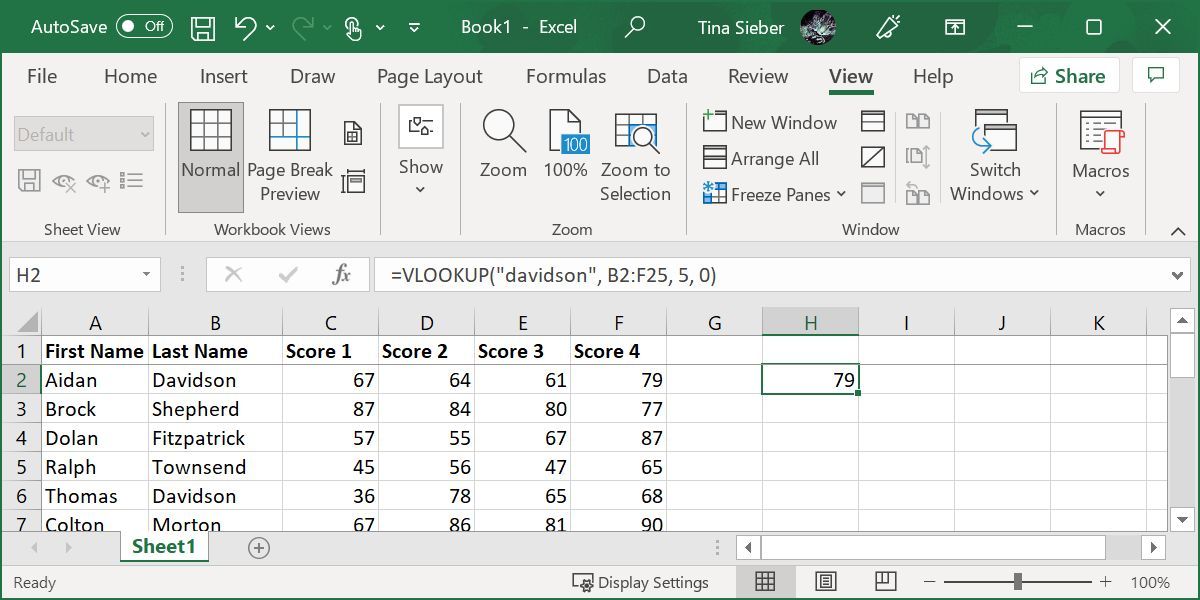
We’ll use the same spreadsheet as before. You can use HLOOKUP to find the score for a specific row. Here’s how we’ll do it:

 =HLOOKUP("Score 4"

As you can see in the image below, the score is returned:

The student in row 6, Thomas Davidson, had a score of 68 on his fourth test.

Notes on HLOOKUP

As with VLOOKUP, the lookup value needs to be in the first row of your table array. This is rarely an issue with HLOOKUP, as you’ll usually be using a column title for a lookup value. HLOOKUP also only returns a single value.

3-4. The INDEX and MATCH Functions

INDEX and MATCH are two different functions, but when they’re used together, they can make searching a large spreadsheet a lot faster. Both functions have drawbacks, but by combining them, we’ll build on the strengths of both.

First, though, the syntax of both functions:

 =INDEX([array], [row_number], [column_number])

[array] is the array in which you’ll be searching.
[row_number] and [column_number] can be used to narrow your search (we’ll take a look at that in a moment).

 =MATCH([lookup_value], [lookup_array], [match_type])

[lookup_value] is a search term that can be a string or a number.
[lookup_array] is the array in which Microsoft Excel will look for the search term.
[match_type] is an optional argument that can be 1, 0, or -1. 1 will return the largest value that is smaller than or equal to your search term. 0 will only return your exact term, and -1 will return the smallest value that is greater than or equal to your search term.

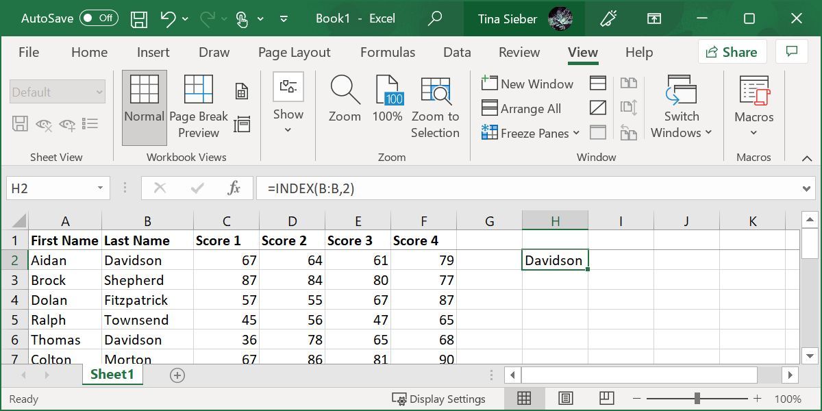
It might not be clear how we’re going to use these two functions together, so I’ll lay it out here. MATCH takes a search term and returns a cell reference. In the image below, you can see that in a search for the last name «Davidson» in column B, MATCH returns 2.

INDEX, on the other hand, does the opposite: it takes a cell reference and returns the value in it. You can see here that, when told to return the second row of column B, INDEX returns «Davidson,» the value from row 2.

What we’re going to do is combine the two so that MATCH returns a cell reference and INDEX uses that reference to look up the value in a cell. Let’s say you remember that there was a student whose last name was Townsend, and you want to see what this student’s fourth score was. Here’s the formula we’ll use:

 =INDEX(F:F, MATCH("Townsend", B:B, 0))

You’ll notice that the match type is set to 0 here. When you’re looking for a string, that’s what you’ll want to use. Here’s what we get when we run that function:

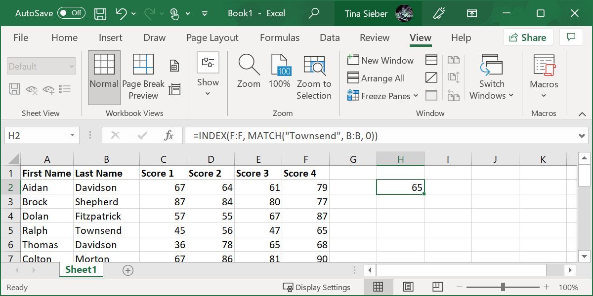
As you can see from the inset, Ralph Townsend scored a 68 in his fourth test, the number that appears when we run the function. This may not seem all that useful when you can just look a few columns over, but imagine how much time you’d save if you had to do it 50 times on a large database spreadsheet that contained several hundred columns!

5. The FIND Function

An article on finding something in Excel wouldn’t be complete without the FIND function. But it might not be what you expect. You can use Excel’s FIND function to identify the position of a string of text within another string of text.

Let’s say, we wanted to find the first occurrence of the letter «x» in the phrase «The brown fox jumped over the fence.» This would be our function:

 =FIND("x", "The brown fox jumped over the fence")

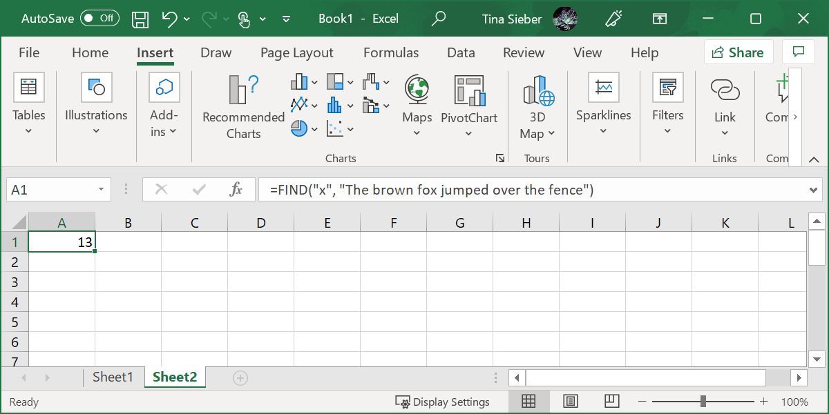
The resulting number represents the position of the queried string. If you’re looking for a multi-character string, let’s say we queried for «fox,» the result would indicate the position of the query’s first character; in this case 11.

Notes on FIND

Like VLOOKUP, HLOOKUP, and other functions, FIND will only identify the first occurrence of a string. Note that FIND is case-sensitive. You can use it to FIND multiple characters. And while we used a letter in our example, it also works with numbers.

On its own, this function might not seem very useful, but it comes into its own when you start nesting functions. For example, you could use your FIND result to split a string of text at the position corresponding to the string identified with FIND.

FIND vs. SEARCH

We can’t cover FIND without mentioning the SEARCH function. Well, it’s essentially the same as FIND, except that it’s not case-sensitive. It also allows wildcards, meaning you can search for matches that aren’t exact.

Excel supports three wildcards:

Asterisk (*), which is a placeholder for any number of characters, including zero.
Question mark (?), which can replace any one character.
Tilde (~), which turns the wildcards «asterisk» and «question mark» into literal characters, meaning it cancels their wildcard function. You’d use it as ~* or ~?.

6. The XLOOKUP Function

XLOOKUP is a new function designed to replace VLOOKUP. Like VLOOKUP, you can use it to find things in a table or range by searching for a known value. It differs from VLOOKUP in that it lets you look up values located in columns to the left or right of the queried value; with VLOOKUP you can only ever find data to the right of the queried column.

Here’s the syntax of the function:

=XLOOKUP(lookup_value, lookup_array, return_array, [if_not_found], [match_mode], [search_mode])

[lookup_value] is the value you’re searching for; i.e. your query.
[lookup_array] is the array or range to search.
[return_array] is the array or range to return. This is the first difference from VLOOKUP.
[if_not_found] is an optional argument that returns a message of your choice if no match is found.
[match_mode] is another optional argument that lets you find exact matches (0), the next smaller item (-1), the next larger item (1), or a wildcard match (2).
[search_mode] is optional and lets you control in which order to search. The default (1) starts the search at the first item. You can also start at the last item (-1), perform a binary search that depends on the lookup_array being sorted in ascending (2) or descending (-2) order.

Let’s take our VLOOKUP example and reverse the search order. This should let us find the score of the second student called Davidson. Here’s the formula:

 =XLOOKUP(G2,B2:B25,F2:F25,,,-1)

Note that we’re pulling the name from column G2, rather than writing it directly into the formula. Below is what it looks like.

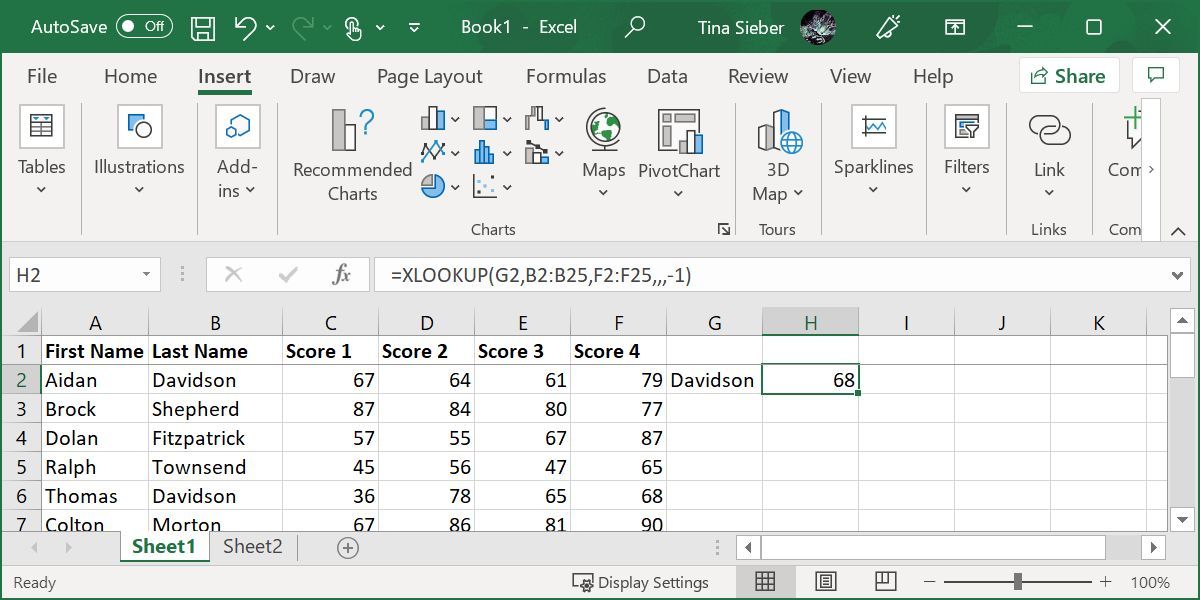
This time, the formula returned Thomas Davidson’s score, rather than that of Aidan Davidson. But it still can’t return more than one result.

Let the Excel Searches Begin

Microsoft Excel has a lot of extremely powerful functions for manipulating data, and the four listed above just scratch the surface. Learning how to use them will make your life much easier.

Источник

Find in Excel (Table of Contents)

Using Find and Select Feature in Excel
FIND Function in Excel
SEARCH Function in Excel

Introduction to Find in Excel

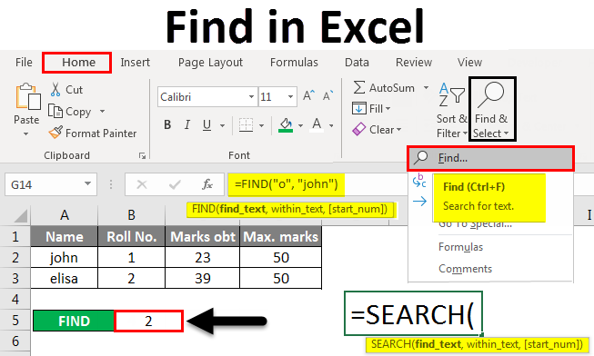
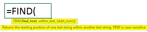
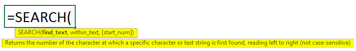
There are two ways to find it in Excel. First, we can use Find by pressing Ctrl + F shortcut keys. Therein Find and Replace box, search the word or field which we want to find in the Find What section. In another way, we can use the FIND function. For this, select the Find function from the insert function and, as per syntax, select the substring from where we need to find it, and choose the word or letter or number which we want to find in the String position. This will return the position of the chosen string from the selected Substring.

Methods to Find in Excel

Below are the different methods to find in excel.

You can download this Find in Excel Template here – Find in Excel Template

Method #1 – Using Find and Select Feature in Excel

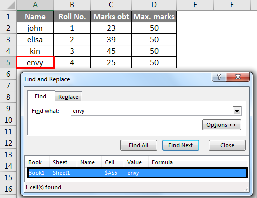
Let’s see How to Find a Number or a Character in Excel using the Find and Select feature in Excel.

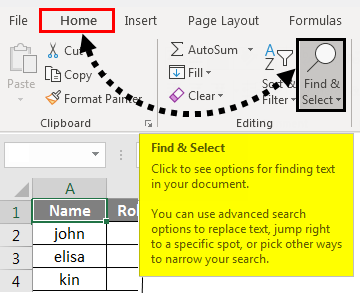
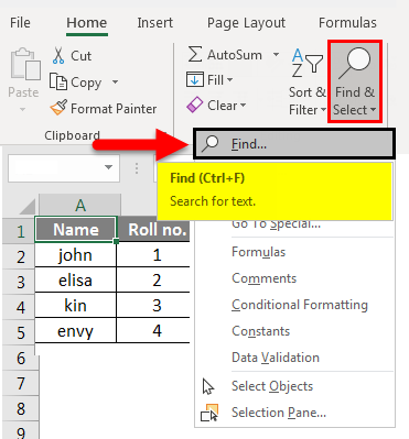
Step 1 – Under the Home tab, in the Editing group, click Find & Select.

Step 2 – To find text or numbers, click Find.

In the Find what box, type the text or character you want to search for, or click the arrow in the Find what box and then click a recent search in the list.

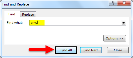
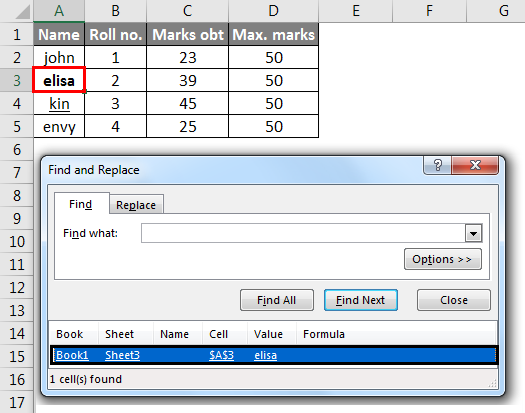
Here, we have a record of marks of four students. Suppose we want to find the text ‘envy’ in this table. For this, we click Find and Select under the Home tab then the Find and Replace dialog box appears. In the Find what box, we enter ‘envy’ then click on Find All. We get the text ‘envy’ is in cell number A5.

You can use wildcard characters, such as an asterisk (*) or a question mark (?), in your search criteria:

Use the asterisk to find any string of characters.

Suppose we want to find text in the table which starts with the letter ‘j’ and ends with the letter ‘n’. In the Find and Replace dialog box, we enter ‘j*n’ in the Find what box, then click on Find All.

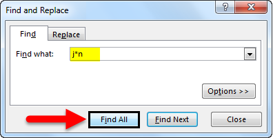
We will get the result as text ‘j*n’(john) is in the cell no. ‘A2’ because we have only one text which starts with ‘j’ and ends with ‘n’ with any number of characters between them.

Use the question mark to find any single character.

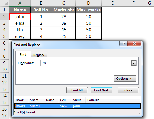
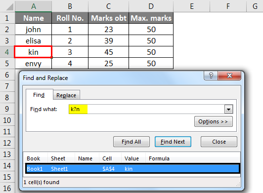
Suppose we want to find text in the table that starts with the letter ‘k’ and ends with the letter ‘n’ with a single character. So, in the Find and Replace dialog box, we enter ‘k?n’ to find what box. Then click on Find All.

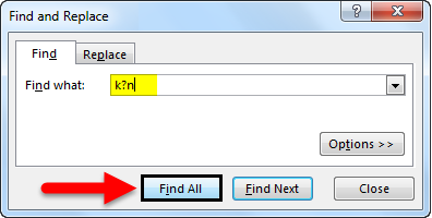
Here, we get the text ‘k?n’(kin) is in cell no. ‘A4’ because we have only one text which starts with ‘k’ and ends with ‘n’ with a single character between them.

Click Options to further define your search if needed.
We can find text or number by changing settings in the Within, Search and Look in the box according to our needs.
To show the working of the above-mentioned options, we took the data as follows.

To search case-sensitive data, select the Match case check box. It gives you output in the case you give input in the Find What box. For example, we have a table of some cars’ names. If you type ‘ferrari’ in the Find What box, then it will find only ‘ferrari’, not ‘Ferrari’.

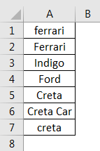
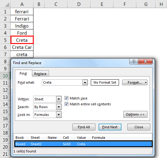
To search for cells that contain just the characters you typed in the Find what box, select the Match entire cell contents checkbox. For example, we have a table of some cars’ names. Type ‘Creta’ in the Find What box.

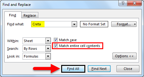
It will then find cells containing exactly ‘Creta’, and cells containing ‘Cretaa’ or ‘Creta car’ will not be found.

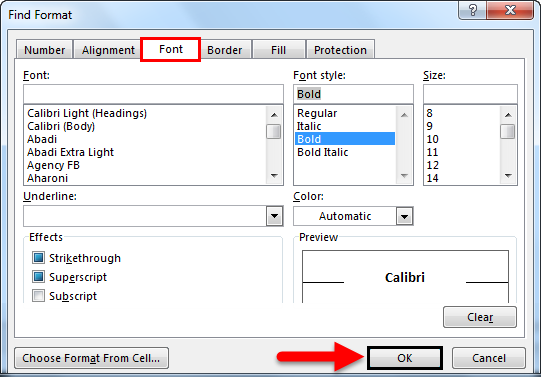
If you want to search for text or numbers with specific formatting, click Format, and then make your selections in the Find Format dialog box according to your need.
Let us click the Font option and select the Bold, and click OK.

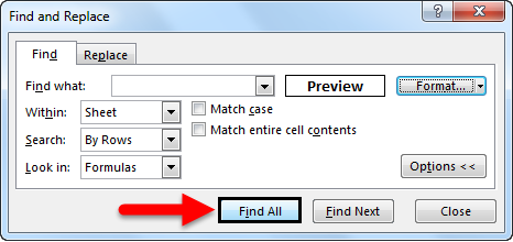
Then, we click on Find All.

We get the value as ‘elisa’, which is in the ‘A3’ cell.

Method #2 – Using FIND Function in Excel

The FIND function in Excel gives the location of a substring within a string.

Syntax For FIND in Excel:

The first two parameters are required, and the last parameter is non-compulsory.

Find_Value: The substring which you want to find.
Within_String: The string in which you want to find the specific substring.
Start_Position: It is a non-compulsory parameter and describes from which position we want to search substring. If you do not describe it, then start the search from the 1^stposition.

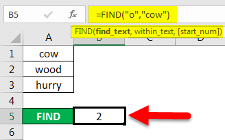
For example =FIND(“o”, “Cow”) gives 2 because “o” is the 2^ndletter in the word “cow“.

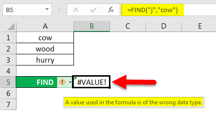
FIND(“j”, “Cow”) gives an error because there is no “j” in “Cow”.

If the Find_Value parameter contains multiple characters, the FIND function gives the location of the first character.

E.g., the formula FIND(“ur”, “hurry”) gives 2 because “u” in the 2^nd letter in the word “hurry”.

If Within_String contains multiple occurrences of Find_Value, the first occurrence is returned. For example, FIND (“o”, “wood”)

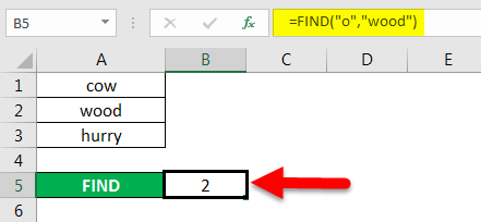
gives 2, which is the location of the first “o” character in the string “wood”.

The Excel FIND function gives the #VALUE! error if:

If Find_Value does not exist in Within_String.
If Start_Position contains multiple characters as compared to Within_String.
If Start_Position either has a zero or negative number.

Method #3 – Using SEARCH Function in Excel

The SEARCH function in Excel is simultaneous to FIND because it also gives the location of a substring in a string.

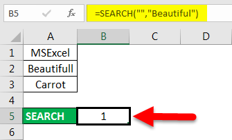
If Find_Value is the blank string “, the Excel FIND formula gives the string’s first character.

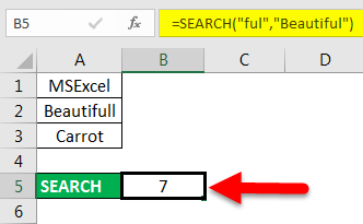
Example =SEARCH (“ful“, “Beautiful) gives 7 because the substring “ful” begins at the 7^th position of the substring “beautiful”.

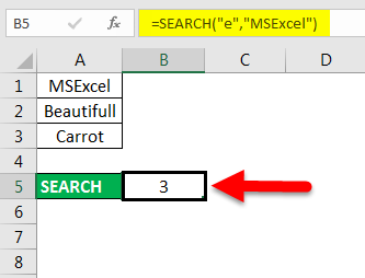
=SEARCH (“e”, “MSExcel”) gives 3 because “e” is the 3rd character in the word “MSExcel” and ignoring the case.

Excel’s SEARCH function gives the #VALUE! error if:

If the value of the Find_Value parameter is not found.
If the Start_Position parameter is superior to the length of Within_String.
If the Start_Position either equal to or less than 0.

Things to Remember About Find in Excel

Asterisk defines a string of characters, and the question mark defines a single character. You can also find asterisks, question marks, and tilde characters (~) in worksheet data by preceding them with a tilde character inside the Find what option.

For example, to find data that contain “*”, you would type ~* as your search criteria.

If you want to find cells that match a specific format, you can delete any criteria in the Find what box and select a specific cell format as an example. Click the arrow next to Format, click Choose Format From Cell, and click the cell with the formatting you want to search for.
MSExcel saves the formatting options you define; you should clear the formatting options from the last search by clicking on an arrow next to Format and then Clear Find Format.
The FIND function is case sensitive and does not allow while using wildcard characters.
The SEARCH function is case-insensitive and allows while using wildcard characters.

Related Excel VBA and Macro Training Materials

The following VBA and Macro training materials may help you better understand and implement the contents below:

Tutorials about general VBA constructs and structures:
- Tutorials for Beginners:
  - Macros.
  - VBA.
- Enable and disable macros.
- The Visual Basic Editor (VBE).
- Procedures:
  - Sub procedures.
  - Function procedures.
- Work with:
  - Objects.
  - Properties.
  - Methods.
  - Variables.
  - Data types.
  - R1C1-style references.
  - Worksheet functions.
  - Loops.
  - Arrays.
- Refer to:
  - Sheets and worksheets.
  - Cell ranges.
Tutorials with practical VBA applications and macro examples:
- Find the last row or last column.
- Set or get a cell’s or cell range’s value.
- Check if a cell is empty.
- Use the VLookup function.
The comprehensive and actionable Books at The Power Spreadsheets Library:
- Excel Macros for Beginners Book Series.
- VBA Fundamentals Book Series.

#1. Excel VBA Find (Cell with) Value in Cell Range

VBA Code to Find (Cell with) Value in Cell Range

To find a cell with a numeric value in a cell range, use the following structure/template in the applicable statement:

CellRangeObject.Find(What:=SearchedValue, After:=SingleCellRangeObject, LookIn:=xlValues, LookAt:=xlWhole, SearchOrder:=XlSearchOrderConstant, SearchDirection:=XlSearchDirectionConstant)

The following Sections describe the main elements in this structure.

CellRangeObject

A Range object representing the cell range you search in.

Find

The Range.Find method:

Finds specific information (the numeric value you search for) in a cell range (CellRangeObject).
Returns a Range object representing the first cell where the information is found.

What:=SearchedValue

The What parameter of the Range.Find method specifies the data to search for.

To find a cell with a numeric value in a cell range, set the What parameter to the numeric value you search for (SearchedValue).

After:=SingleCellRangeObject

The After parameter of the Range.Find method specifies the cell after which the search begins. This must be a single cell in the cell range you search in (CellRangeObject).

If you omit specifying the After parameter, the search begins after the first cell (in the upper left corner) of the cell range you search in (CellRangeObject).

To find a cell with a numeric value in a cell range, set the After parameter to a Range object representing the cell after which the search begins.

LookIn:=xlValues

The LookIn parameter of the Range.Find method:

Specifies the type of data to search in.
Can take any of the built-in constants/values from the XlFindLookIn enumeration.

To find a cell with a numeric value in a cell range, set the LookIn parameter to xlValues. xlValues refers to values.

LookAt:=xlWhole

The LookAt parameter of the Range.Find method:

Specifies against which of the following the data you are searching for is matched:
- The entire/whole searched cell contents.
- Any part of the searched cell contents.
Can take any of the built-in constants/values from the XlLookAt enumeration.

To find a cell with a numeric value in a cell range, set the LookAt parameter to xlWhole. xlWhole matches the data you are searching for against the entire/whole searched cell contents.

SearchOrder:=XlSearchOrderConstant

The SearchOrder parameter of the Range.Find method:

Specifies the order in which the applicable cell range (CellRangeObject) is searched:
- By rows.
- By columns.
Can take any of the built-in constants/values from the XlSearchOrder enumeration.

To find a cell with a numeric value in a cell range, set the SearchOrder parameter to either of the following, as applicable:

xlByRows (SearchOrder:=xlByRows): To search by rows.
xlByColumns (SearchOrder:=xlByColumns): To search by columns.

SearchDirection:=XlSearchDirectionConstant

The SearchDirection parameter of the Range.Find method:

Specifies the search direction:
- Search for the previous match.
- Search for the next match.
Can take any of the built-in constants/values from the XlSearchDirection enumeration.

To find a cell with a numeric value in a cell range, set the SearchDirection parameter to either of the following, as applicable:

xlNext (SearchDirection:=xlNext): To search for the next match.
xlPrevious (SearchDirection:=xlPrevious): To search for the previous match.

Macro Example to Find (Cell with) Value in Cell Range

The following macro (User-Defined Function) example does the following:

Accepts two arguments:
1. MyRange: The cell range you search in.
2. MyValue: The numeric value you search for.
Finds MyValue in MyRange.
Returns a string containing the address (as an A1-style relative reference) of the first cell in the cell range (MyRange) where the numeric value (MyValue) is found.

Function FindValueInCellRange(MyRange As Range, MyValue As Variant) As String
    'Source: https://powerspreadsheets.com/
    'For further information: https://powerspreadsheets.com/excel-vba-find/
    
    'This UDF:
        '(1) Accepts 2 arguments: MyRange and MyValue
        '(2) Finds a value passed as argument (MyValue) in a cell range passed as argument (MyRange)
        '(3) Returns the address (as an A1-style relative reference) of the first cell in the cell range (MyRange) where the value (MyValue) is found
    
    With MyRange
        FindValueInCellRange = .Find(What:=MyValue, After:=.Cells(.Cells.Count), LookIn:=xlValues, LookAt:=xlWhole, SearchOrder:=xlByRows, SearchDirection:=xlNext).Address(RowAbsolute:=False, ColumnAbsolute:=False)
    End With
    
End Function

Effects of Executing Macro Example to Find (Cell with) Value in Cell Range

The following image illustrates the effects of using the macro (User-Defined Function) example. In this example:

Columns A through H (cells A6 to H30) contain randomly generated values.
Cell J7 contains the searched value (41).
Cell K7 contains the worksheet formula that works with the macro (User-Defined Function) example. This worksheet formula returns the address (as an A1-style relative reference) of the first cell in the cell range (MyRange) where the numeric value (MyValue) is found. This is cell B11.
Cell L7 displays the worksheet formula used in cell K7 (=FindValueInCellRange(A6:H30,J7)).
- The cell range where the search is carried out contains cells A6 to H30 (A6:H30).
- The searched value is stored in cell J7 (J7).

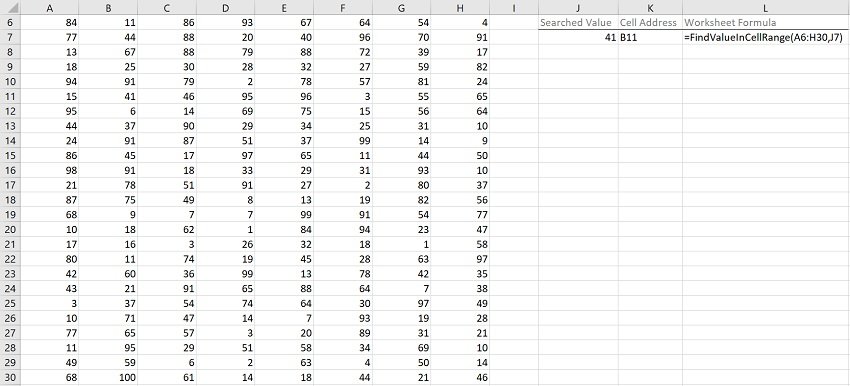
Example: Find value in cell range with VBA macros

#2. Excel VBA Find (Cell with) Value in Table

VBA Code to Find (Cell with) Value in Table

To find a cell with a numeric value in an Excel Table, use the following structure/template in the applicable statement:

ListObjectObject.DataBodyRange.Find(What:=SearchedValue, After:=SingleCellRangeObject, LookIn:=xlValues, LookAt:=xlWhole, SearchOrder:=XlSearchOrderConstant, SearchDirection:=XlSearchDirectionConstant)

The following Sections describe the main elements in this structure.

ListObjectObject

A ListObject object representing the Excel Table you search in.

DataBodyRange

The ListObject.DataBodyRange property returns a Range object representing the cell range containing an Excel Table’s values (excluding the headers).

Find

The Range.Find method:

Finds specific information (the numeric value you search for) in a cell range (containing the applicable Excel Table’s values).
Returns a Range object representing the first cell where the information is found.

What:=SearchedValue

The What parameter of the Range.Find method specifies the data to search for.

To find a cell with a numeric value in an Excel Table, set the What parameter to the numeric value you search for (SearchedValue).

After:=SingleCellRangeObject

The After parameter of the Range.Find method specifies the cell after which the search begins. This must be a single cell in the cell range you search in (containing the applicable Excel Table’s values).

If you omit specifying the After parameter, the search begins after the first cell (in the upper left corner) of the cell range you search in (containing the applicable Excel Table’s values).

To find a cell with a numeric value in an Excel Table, set the After parameter to a Range object representing the cell after which the search begins.

LookIn:=xlValues

The LookIn parameter of the Range.Find method:

Specifies the type of data to search in.
Can take any of the built-in constants/values from the XlFindLookIn enumeration.

To find a cell with a numeric value in an Excel Table, set the LookIn parameter to xlValues. xlValues refers to values.

LookAt:=xlWhole

The LookAt parameter of the Range.Find method:

Specifies against which of the following the data you are searching for is matched:
- The entire/whole searched cell contents.
- Any part of the searched cell contents.
Can take any of the built-in constants/values from the XlLookAt enumeration.

To find a cell with a numeric value in an Excel Table, set the LookAt parameter to xlWhole. xlWhole matches the data you are searching for against the entire/whole searched cell contents.

SearchOrder:=XlSearchOrderConstant

The SearchOrder parameter of the Range.Find method:

Specifies the order in which the applicable cell range (containing the applicable Excel Table’s values) is searched:
- By rows.
- By columns.
Can take any of the built-in constants/values from the XlSearchOrder enumeration.

To find a cell with a numeric value in an Excel Table, set the SearchOrder parameter to either of the following, as applicable:

xlByRows (SearchOrder:=xlByRows): To search by rows.
xlByColumns (SearchOrder:=xlByColumns): To search by columns.

SearchDirection:=XlSearchDirectionConstant

The SearchDirection parameter of the Range.Find method:

Specifies the search direction:
- Search for the previous match.
- Search for the next match.
Can take any of the built-in constants/values from the XlSearchDirection enumeration.

To find a cell with a numeric value in an Excel Table, set the SearchDirection parameter to either of the following, as applicable:

xlNext (SearchDirection:=xlNext): To search for the next match.
xlPrevious (SearchDirection:=xlPrevious): To search for the previous match.

Macro Example to Find (Cell with) Value in Table

The following macro (User-Defined Function) example does the following:

Accepts 3 arguments:
1. MyWorksheetName: The name of the worksheet where the Excel Table you search in is stored.
2. MyValue: The numeric value you search for.
3. MyTableIndex: The index number of the Excel Table (stored in the worksheet named MyWorksheetName) you search in. MyTableIndex is an optional argument with a default value of 1.
Finds MyValue in the applicable Excel Table’s values (excluding the headers).
Returns a string containing the address (as an A1-style relative reference) of the first cell in the applicable Excel Table where the numeric value (MyValue) is found.

Function FindValueInTable(MyWorksheetName As String, MyValue As Variant, Optional MyTableIndex As Long = 1) As String
    'Source: https://powerspreadsheets.com/
    'For further information: https://powerspreadsheets.com/excel-vba-find/
    
    'This UDF:
        '(1) Accepts 3 arguments: MyWorksheetName, MyValue and MyTableIndex
        '(2) Finds a value passed as argument (MyValue) in an Excel Table stored in a worksheet whose name is passed as argument (MyWorksheetName). The index number of the Excel Table is either:
            '(1) Passed as an argument (MyTableIndex); or
            '(2) Assumed to be 1 (if MyTableIndex is omitted)
        '(3) Returns the address (as an A1-style relative reference) of the first cell in the Excel Table (stored in the MyWorksheetName worksheet and whose index is MyTableIndex) where the value (MyValue) is found
    
    With ThisWorkbook.Worksheets(MyWorksheetName).ListObjects(MyTableIndex).DataBodyRange
        FindValueInTable = .Find(What:=MyValue, After:=.Cells(.Cells.Count), LookIn:=xlValues, LookAt:=xlWhole, SearchOrder:=xlByRows, SearchDirection:=xlNext).Address(RowAbsolute:=False, ColumnAbsolute:=False)
    End With
    
End Function

Effects of Executing Macro Example to Find (Cell with) Value in Table

The following image illustrates the effects of using the macro (User-Defined Function) example. In this example:

Columns A through H (cells A6 to H31) contain an Excel Table with randomly generated values.
Cell J7 contains the searched value (41).
Cell K7 contains the worksheet formula that works with the macro (User-Defined Function) example. This worksheet formula returns the address (as an A1-style relative reference) of the first cell in the Excel Table where the numeric value (MyValue) is found. This is cell B12.
Cell L7 displays the worksheet formula used in cell K7 (=FindValueInTable(“Find Value in Table”,J7)).
- The name of the worksheet where the Excel Table is stored is “Find Value in Table” (“Find Value in Table”).
- The searched value is stored in cell J7 (J7).
- The index number of the Excel Table is 1 (by default).

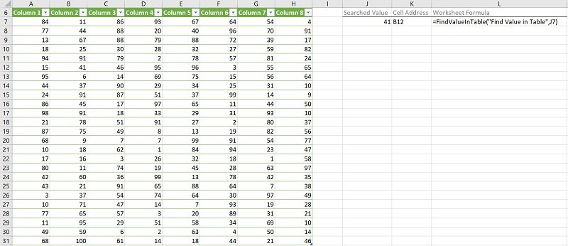
Example: Find value in table with VBA macros

#3. Excel VBA Find (Cell with) Value in Column

VBA Code to Find (Cell with) Value in Column

To find a cell with a numeric value in a column, use the following structure/template in the applicable statement:

RangeObjectColumn.Find(What:=SearchedValue, After:=SingleCellRangeObject, LookIn:=xlValues, LookAt:=xlWhole, SearchOrder:=xlByRows, SearchDirection:=XlSearchDirectionConstant)

The following Sections describe the main elements in this structure.

RangeObjectColumn

A Range object representing the column you search in.

Find

The Range.Find method:

Finds specific information (the numeric value you search for) in a cell range (RangeObjectColumn).
Returns a Range object representing the first cell where the information is found.

What:=SearchedValue

The What parameter of the Range.Find method specifies the data to search for.

To find a cell with a numeric value in a column, set the What parameter to the numeric value you search for (SearchedValue).

After:=SingleCellRangeObject

The After parameter of the Range.Find method specifies the cell after which the search begins. This must be a single cell in the column you search in (RangeObjectColumn).

If you omit specifying the After parameter, the search begins after the first cell of the column you search in (RangeObjectColumn).

To find a cell with a numeric value in a column, set the After parameter to a Range object representing the cell after which the search begins.

LookIn:=xlValues

The LookIn parameter of the Range.Find method:

Specifies the type of data to search in.
Can take any of the built-in constants/values from the XlFindLookIn enumeration.

To find a cell with a numeric value in a column, set the LookIn parameter to xlValues. xlValues refers to values.

LookAt:=xlWhole

The LookAt parameter of the Range.Find method:

Specifies against which of the following the data you are searching for is matched:
- The entire/whole searched cell contents.
- Any part of the searched cell contents.
Can take any of the built-in constants/values from the XlLookAt enumeration.

To find a cell with a numeric value in a column, set the LookAt parameter to xlWhole. xlWhole matches the data you are searching for against the entire/whole searched cell contents.

SearchOrder:=xlByRows

The SearchOrder parameter of the Range.Find method:

Specifies the order in which the applicable column (RangeObjectColumn) is searched:
- By rows.
- By columns.
Can take any of the built-in constants/values from the XlSearchOrder enumeration.

To find a cell with a numeric value in a column, set the SearchOrder parameter to xlByRows. xlByRows results in the Range.Find method searching by rows.

SearchDirection:=XlSearchDirectionConstant

The SearchDirection parameter of the Range.Find method:

Specifies the search direction:
- Search for the previous match.
- Search for the next match.
Can take any of the built-in constants/values from the XlSearchDirection enumeration.

To find a cell with a numeric value in a column, set the SearchDirection parameter to either of the following, as applicable:

xlNext (SearchDirection:=xlNext): To search for the next match.
xlPrevious (SearchDirection:=xlPrevious): To search for the previous match.

Macro Example to Find (Cell with) Value in Column

The following macro (User-Defined Function) example does the following:

Accepts two arguments:
1. MyColumn: The column you search in.
2. MyValue: The numeric value you search for.
Finds MyValue in MyColumn.
Returns a string containing the address (as an A1-style relative reference) of the first cell in the column (MyColumn) where the numeric value (MyValue) is found.

Function FindValueInColumn(MyColumn As Range, MyValue As Variant) As String
    'Source: https://powerspreadsheets.com/
    'For further information: https://powerspreadsheets.com/excel-vba-find/
    
    'This UDF:
        '(1) Accepts 2 arguments: MyColumn and MyValue
        '(2) Finds a value passed as argument (MyValue) in a column passed as argument (MyColumn)
        '(3) Returns the address (as an A1-style relative reference) of the first cell in the column (MyColumn) where the value (MyValue) is found
    
    With MyColumn
        FindValueInColumn = .Find(What:=MyValue, After:=.Cells(.Cells.Count), LookIn:=xlValues, LookAt:=xlWhole, SearchOrder:=xlByRows, SearchDirection:=xlNext).Address(RowAbsolute:=False, ColumnAbsolute:=False)
    End With
    
End Function

Effects of Executing Macro Example to Find (Cell with) Value in Column

The following image illustrates the effects of using the macro (User-Defined Function) example. In this example:

Column A (cells A6 to A31) contains randomly generated values.
Cell C7 contains the searched value (90).
Cell D7 contains the worksheet formula that works with the macro (User-Defined Function) example. This worksheet formula returns the address (as an A1-style relative reference) of the first cell in the column (MyColumn) where the numeric value (MyValue) is found. This is cell A13.
Cell E7 displays the worksheet formula used in cell D7 (=FindValueInColumn(A:A,C7)).
- The column where the search is carried out is column A (A:A).
- The searched value is stored in cell C7 (C7).

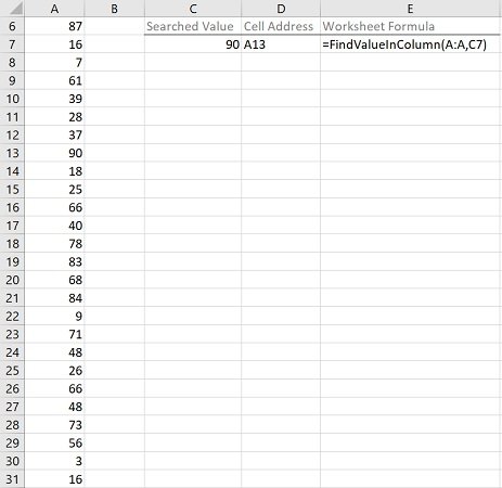
#4. Excel VBA Find (Cell with) Value in Table Column

VBA Code to Find (Cell with) Value in Table Column

To find a cell with a numeric value in an Excel Table column, use the following structure/template in the applicable statement:

ListColumnObject.DataBodyRange.Find(What:=SearchedValue, After:=SingleCellRangeObject, LookIn:=xlValues, LookAt:=xlWhole, SearchOrder:=XlSearchOrderConstant, SearchDirection:=XlSearchDirectionConstant)

The following Sections describe the main elements in this structure.

ListColumnObject

A ListColumn object representing the Excel Table column you search in.

DataBodyRange

The ListColumn.DataBodyRange property returns a Range object representing the cell range containing an Excel Table column’s values (excluding the header).

Find

The Range.Find method:

Finds specific information (the numeric value you search for) in a cell range (containing the applicable Excel Table column’s values).
Returns a Range object representing the first cell where the information is found.

What:=SearchedValue

The What parameter of the Range.Find method specifies the data to search for.

To find a cell with a numeric value in an Excel Table column, set the What parameter to the numeric value you search for (SearchedValue).

After:=SingleCellRangeObject

If you omit specifying the After parameter, the search begins after the first cell of the cell range you search in (containing the applicable Excel Table column’s values).

To find a cell with a numeric value in an Excel Table column, set the After parameter to a Range object representing the cell after which the search begins.

LookIn:=xlValues

The LookIn parameter of the Range.Find method:

Specifies the type of data to search in.
Can take any of the built-in constants/values from the XlFindLookIn enumeration.

To find a cell with a numeric value in an Excel Table column, set the LookIn parameter to xlValues. xlValues refers to values.

LookAt:=xlWhole

The LookAt parameter of the Range.Find method:

Specifies against which of the following the data you are searching for is matched:
- The entire/whole searched cell contents.
- Any part of the searched cell contents.
Can take any of the built-in constants/values from the XlLookAt enumeration.

To find a cell with a numeric value in an Excel Table column, set the LookAt parameter to xlWhole. xlWhole matches the data you are searching for against the entire/whole searched cell contents.

SearchOrder:=XlSearchOrderConstant

The SearchOrder parameter of the Range.Find method:

Specifies the order in which the applicable cell range (containing the applicable Excel Table column’s values) is searched:
- By rows.
- By columns.
Can take any of the built-in constants/values from the XlSearchOrder enumeration.

To find a cell with a numeric value in an Excel Table column, set the SearchOrder parameter to either of the following, as applicable:

xlByRows (SearchOrder:=xlByRows): To search by rows.
xlByColumns (SearchOrder:=xlByColumns): To search by columns.

SearchDirection:=XlSearchDirectionConstant

The SearchDirection parameter of the Range.Find method:

Specifies the search direction:
- Search for the previous match.
- Search for the next match.
Can take any of the built-in constants/values from the XlSearchDirection enumeration.

To find a cell with a numeric value in an Excel Table column, set the SearchDirection parameter to either of the following, as applicable:

xlNext (SearchDirection:=xlNext): To search for the next match.
xlPrevious (SearchDirection:=xlPrevious): To search for the previous match.

Macro Example to Find (Cell with) Value in Table Column

The following macro (User-Defined Function) example does the following:

Accepts 4 arguments:
1. MyWorksheetName: The name of the worksheet where the Excel Table (containing the column you search in) is stored.
2. MyColumnIndex: The index/column number of the column you search in (in the applicable Excel Table).
3. MyValue: The numeric value you search for.
4. MyTableIndex: The index number of the Excel Table (stored in the worksheet named MyWorksheetName) containing the column you search in. MyTableIndex is an optional argument with a default value of 1.
Finds MyValue in the applicable Excel Table column’s values (excluding the header).
Returns a string containing the address (as an A1-style relative reference) of the first cell in the applicable Excel Table column where the numeric value (MyValue) is found.

Function FindValueInTableColumn(MyWorksheetName As String, MyColumnIndex As Long, MyValue As Variant, Optional MyTableIndex As Long = 1) As String
    'Source: https://powerspreadsheets.com/
    'For further information: https://powerspreadsheets.com/excel-vba-find/
    
    'This UDF:
        '(1) Accepts 4 arguments: MyWorksheetName, MyColumnIndex, MyValue and MyTableIndex
        '(2) Finds a value passed as argument (MyValue) in an Excel Table column, where:
            '(1) The table column's index is passed as argument (MyColumnIndex); and
            '(2) The Excel Table is stored in a worksheet whose name is passed as argument (MyWorksheetName). The index number of the Excel Table is either:
                '(1) Passed as an argument (MyTableIndex); or
                '(2) Assumed to be 1 (if MyTableIndex is omitted)
        '(3) Returns the address (as an A1-style relative reference) of the first cell in the applicable Excel Table column where the value (MyValue) is found
    
    With ThisWorkbook.Worksheets(MyWorksheetName).ListObjects(MyTableIndex).ListColumns(MyColumnIndex).DataBodyRange
        FindValueInTableColumn = .Find(What:=MyValue, After:=.Cells(.Cells.Count), LookIn:=xlValues, LookAt:=xlWhole, SearchOrder:=xlByRows, SearchDirection:=xlNext).Address(RowAbsolute:=False, ColumnAbsolute:=False)
    End With
    
End Function

Effects of Executing Macro Example to Find (Cell with) Value in Table Column

The following image illustrates the effects of using the macro (User-Defined Function) example. In this example:

Columns A through H (cells A6 to H31) contain an Excel Table with randomly generated values. Cells in the first row (row 7) contain the searched value (90), except for the cell in the searched column (Column 3).
Cell J7 contains the searched value (90).
Cell K7 contains the worksheet formula that works with the macro (User-Defined Function) example. This worksheet formula returns the address (as an A1-style relative reference) of the first cell in the applicable Excel Table column (Column 3) where the numeric value (MyValue) is found. This is cell C14.
Cell L7 displays the worksheet formula used in cell K7 (=FindValueInTableColumn(“Find Value in Table Column”,3, J7)).
- The name of the worksheet where the Excel Table is stored is “Find Value in Table Column” (“Find Value in Table Column”).
- The index number of the Excel Table column is 3 (3).
- The searched value is stored in cell J7 (J7).
- The index number of the Excel Table is 1 (by default).

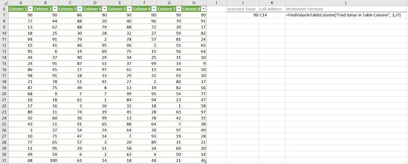
Example: Find value in table column with VBA macros

#5. Excel VBA Find Minimum Value in Cell Range

VBA Code to Find Minimum Value in Cell Range

To find the minimum value in a cell range, use the following structure/template in the applicable statement:

Application.Min(CellRangeObject)

The following Sections describe the main elements in this structure.

Application.Min

The WorksheetFunction.Min method returns the minimum value in a set of values.

CellRangeObject

The WorksheetFunction.Min method accepts up to thirty parameters (Arg1 to Arg30). These are the values for which you want to find the minimum value.

To find the minimum value in a cell range, pass a Range object (CellRangeObject) representing the cell range whose minimum value you want to find as method parameter.

Macro Example to Find Minimum Value in Cell Range

The following macro (User-Defined Function) example does the following:

Accepts 1 argument (MyRange): The cell range whose minimum value you search for.
Finds and returns the minimum value in the cell range (MyRange).

Function FindMinimumValueInCellRange(MyRange As Range) As Double
    'Source: https://powerspreadsheets.com/
    'For further information: https://powerspreadsheets.com/excel-vba-find/
    
    'This UDF:
        '(1) Accepts 1 argument: MyRange
        '(2) Finds the minimum value in the cell range passed as argument (MyRange)
    
    FindMinimumValueInCellRange = Application.Min(MyRange)

End Function

Effects of Executing Macro Example to Find Minimum Value in Cell Range

The following image illustrates the effects of using the macro (User-Defined Function) example. In this example:

Columns A through H (cells A6 to H30) contain randomly generated values.
Cell J7 contains the worksheet formula that works with the macro (User-Defined Function) example. This worksheet formula returns the minimum value in the cell range (MyRange). This is the number 1.
Cell K7 displays the worksheet formula used in cell J7 (=FindMinimumValueInCellRange(A6:H30)). The cell range where the search is carried out contains cells A6 to H30 (A6:H30).

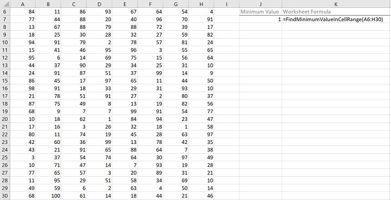
Example: Find minimum value in cell range with VBA macros

#6. Excel VBA Find (Cell with) String (or Text) in Cell Range

VBA Code to Find (Cell with) String (or Text) in Cell Range

To find a cell with a string (or text) in a cell range, use the following structure/template in the applicable statement:

CellRangeObject.Find(What:=SearchedString, After:=SingleCellRangeObject, LookIn:=XlFindLookInConstant, LookAt:=XlLookAtConstant, SearchOrder:=XlSearchOrderConstant, SearchDirection:=XlSearchDirectionConstant, MatchCase:=BooleanValue)

The following Sections describe the main elements in this structure.

CellRangeObject

A Range object representing the cell range you search in.

Find

The Range.Find method:

Finds specific information (the string or text you search for) in a cell range (CellRangeObject).
Returns a Range object representing the first cell where the information is found.

What:=SearchedString

The What parameter of the Range.Find method specifies the data to search for.

To find a cell with a string (or text) in a cell range, set the What parameter to the string (or text) you search for (SearchedString).

After:=SingleCellRangeObject

The After parameter of the Range.Find method specifies the cell after which the search begins. This must be a single cell in the cell range you search in (CellRangeObject).

If you omit specifying the After parameter, the search begins after the first cell (in the upper left corner) of the cell range you search in (CellRangeObject).

To find a cell with a string (or text) in a cell range, set the After parameter to a Range object representing the cell after which the search begins.

LookIn:=XlFindLookInConstant

The LookIn parameter of the Range.Find method:

Specifies the type of data to search in.
Can take any of the built-in constants/values from the XlFindLookIn enumeration.

To find a cell with a string (or text) in a cell range, set the LookIn parameter to either of the following, as applicable:

xlFormulas (LookIn:=xlFormulas): To search in the applicable cell range’s formulas.
xlValues (LookIn:=xlValues): To search in the applicable cell range’s values.

LookAt:=XlLookAtConstant

The LookAt parameter of the Range.Find method:

Specifies against which of the following the data you are searching for is matched:
- The entire/whole searched cell contents.
- Any part of the searched cell contents.
Can take any of the built-in constants/values from the XlLookAt enumeration.

To find a cell with a string (or text) in a cell range, set the LookAt parameter to either of the following, as applicable:

xlWhole (LookAt:=xlWhole): To match against the entire/whole searched cell contents.
xlPart (LookAt:=xlPart): To match against any part of the searched cell contents.

SearchOrder:=XlSearchOrderConstant

The SearchOrder parameter of the Range.Find method:

Specifies the order in which the applicable cell range (CellRangeObject) is searched:
- By rows.
- By columns.
Can take any of the built-in constants/values from the XlSearchOrder enumeration.

To find a cell with a string (or text) in a cell range, set the SearchOrder parameter to either of the following, as applicable:

xlByRows (SearchOrder:=xlByRows): To search by rows.
xlByColumns (SearchOrder:=xlByColumns): To search by columns.

SearchDirection:=XlSearchDirectionConstant

The SearchDirection parameter of the Range.Find method:

Specifies the search direction:
- Search for the previous match.
- Search for the next match.
Can take any of the built-in constants/values from the XlSearchDirection enumeration.

To find a cell with a string (or text) in a cell range, set the SearchDirection parameter to either of the following, as applicable:

xlNext (SearchDirection:=xlNext): To search for the next match.
xlPrevious (SearchDirection:=xlPrevious): To search for the previous match.

MatchCase:=BooleanValue

The MatchCase parameter of the Range.Find method specifies whether the search is:

Case-sensitive; or
Case-insensitive.

The default value of the MatchCase parameter is False.

To find a cell with a string (or text) in a cell range, set the MatchCase parameter to either of the following, as applicable:

True (MatchCase:=True): To carry out a case-sensitive search.
False (MatchCase:=False): To carry out a case-insensitive search.

Macro Example to Find (Cell with) String (or Text) in Cell Range

The following macro (User-Defined Function) example does the following:

Accepts two arguments:
1. MyRange: The cell range you search in.
2. MyString: The string (or text) you search for.
Finds MyString in MyRange. The search is case-insensitive.
Returns a string containing the address (as an A1-style relative reference) of the first cell in the cell range (MyRange) where the string or text (MyString) is found.

Function FindStringInCellRange(MyRange As Range, MyString As Variant) As String
    'Source: https://powerspreadsheets.com/
    'For further information: https://powerspreadsheets.com/excel-vba-find/
    
    'This UDF:
        '(1) Accepts 2 arguments: MyRange and MyString
        '(2) Finds a string passed as argument (MyString) in a cell range passed as argument (MyRange). The search is case-insensitive
        '(3) Returns the address (as an A1-style relative reference) of the first cell in the cell range (MyRange) where the string (MyString) is found
    
    With MyRange
        FindStringInCellRange = .Find(What:=MyString, After:=.Cells(.Cells.Count), LookIn:=xlValues, LookAt:=xlWhole, SearchOrder:=xlByRows, SearchDirection:=xlNext, MatchCase:=False).Address(RowAbsolute:=False, ColumnAbsolute:=False)
    End With
    
End Function

Effects of Executing Macro Example to Find (Cell with) String (or Text) in Cell Range

The following image illustrates the effects of using the macro (User-Defined Function) example. In this example:

Columns A through H (cells A6 to H30) contain randomly generated words.
Cell J7 contains the searched string or text (Excel).
Cell K7 contains the worksheet formula that works with the macro (User-Defined Function) example. This worksheet formula returns the address (as an A1-style relative reference) of the first cell in the cell range (MyRange) where the string or text (MyString) is found. This is cell F20.
Cell L7 displays the worksheet formula used in cell K7 (=FindStringInCellRange(A6:H30,J7)).
- The cell range where the search is carried out contains cells A6 to H30 (A6:H30).
- The searched string or text is stored in cell J7 (J7).

Example: Find String in cell range with VBA macros

#7. Excel VBA Find (Cell with) String (or Text) in Column

VBA Code to Find (Cell with) String (or Text) in Column

To find a cell with a string (or text) in a column, use the following structure/template in the applicable statement:

RangeObjectColumn.Find(What:=SearchedString, After:=SingleCellRangeObject, LookIn:=XlFindLookInConstant, LookAt:=XlLookAtConstant, SearchOrder:=xlByRows, SearchDirection:=XlSearchDirectionConstant, MatchCase:=BooleanValue)

The following Sections describe the main elements in this structure.

RangeObjectColumn

A Range object representing the column you search in.

Find

The Range.Find method:

Finds specific information (the string or text you search for) in a cell range (RangeObjectColumn).
Returns a Range object representing the first cell where the information is found.

What:=SearchedString

The What parameter of the Range.Find method specifies the data to search for.

To find a cell with a string (or text) in a column, set the What parameter to the string (or text) you search for (SearchedString).

After:=SingleCellRangeObject

The After parameter of the Range.Find method specifies the cell after which the search begins. This must be a single cell in the column you search in (RangeObjectColumn).

If you omit specifying the After parameter, the search begins after the first cell of the column you search in (RangeObjectColumn).

To find a cell with a string (or text) in a column, set the After parameter to a Range object representing the cell after which the search begins.

LookIn:=XlFindLookInConstant

The LookIn parameter of the Range.Find method:

Specifies the type of data to search in.
Can take any of the built-in constants/values from the XlFindLookIn enumeration.

To find a cell with a string (or text) in a column, set the LookIn parameter to either of the following, as applicable:

xlFormulas (LookIn:=xlFormulas): To search in the applicable column’s formulas.
xlValues (LookIn:=xlValues): To search in the applicable column’s values.

LookAt:=XlLookAtConstant

The LookAt parameter of the Range.Find method:

Specifies against which of the following the data you are searching for is matched:
- The entire/whole searched cell contents.
- Any part of the searched cell contents.
Can take any of the built-in constants/values from the XlLookAt enumeration.

To find a cell with a string (or text) in a column, set the LookAt parameter to either of the following, as applicable:

xlWhole (LookAt:=xlWhole): To match against the entire/whole searched cell contents.
xlPart (LookAt:=xlPart): To match against any part of the searched cell contents.

SearchOrder:=xlByRows

The SearchOrder parameter of the Range.Find method:

Specifies the order in which the applicable column (RangeObjectColumn) is searched:
- By rows.
- By columns.
Can take any of the built-in constants/values from the XlSearchOrder enumeration.

To find a cell with a string (or text) in a column, set the SearchOrder parameter to xlByRows. xlByRows results in the Range.Find method searching by rows.

SearchDirection:=XlSearchDirectionConstant

The SearchDirection parameter of the Range.Find method:

Specifies the search direction:
- Search for the previous match.
- Search for the next match.
Can take any of the built-in constants/values from the XlSearchDirection enumeration.

To find a cell with a string (or text) in a column, set the SearchDirection parameter to either of the following, as applicable:

xlNext (SearchDirection:=xlNext): To search for the next match.
xlPrevious (SearchDirection:=xlPrevious): To search for the previous match.

MatchCase:=BooleanValue

The MatchCase parameter of the Range.Find method specifies whether the search is:

Case-sensitive; or
Case-insensitive.

The default value of the MatchCase parameter is False.

To find a cell with a string (or text) in a column, set the MatchCase parameter to either of the following, as applicable:

True (MatchCase:=True): To carry out a case-sensitive search.
False (MatchCase:=False): To carry out a case-insensitive search.

Macro Example to Find (Cell with) String (or Text) in Column

The following macro (User-Defined Function) example does the following:

Accepts two arguments:
1. MyColumn: The column you search in.
2. MyString: The string (or text) you search for.
Finds MyString in MyColumn. The search is case-insensitive.
Returns a string containing the address (as an A1-style relative reference) of the first cell in the column (MyColumn) where the string or text (MyString) is found.

Function FindStringInColumn(MyColumn As Range, MyString As Variant) As String
    'Source: https://powerspreadsheets.com/
    'For further information: https://powerspreadsheets.com/excel-vba-find/
    
    'This UDF:
        '(1) Accepts 2 arguments: MyColumn and MyString
        '(2) Finds a string passed as argument (MyString) in a column passed as argument (MyColumn). The search is case-insensitive
        '(3) Returns the address (as an A1-style relative reference) of the first cell in the column (MyColumn) where the string (MyString) is found
    
    With MyColumn
        FindStringInColumn = .Find(What:=MyString, After:=.Cells(.Cells.Count), LookIn:=xlValues, LookAt:=xlWhole, SearchOrder:=xlByRows, SearchDirection:=xlNext, MatchCase:=False).Address(RowAbsolute:=False, ColumnAbsolute:=False)
    End With
    
End Function

Effects of Executing Macro Example to Find (Cell with) String (or Text) in Column

The following image illustrates the effects of using the macro (User-Defined Function) example. In this example:

Column A (cells A6 to A30) contains randomly generated words.
Cell C7 contains the searched string or text (Excel).
Cell D7 contains the worksheet formula that works with the macro (User-Defined Function) example. This worksheet formula returns the address (as an A1-style relative reference) of the first cell in the column (MyColumn) where the string or text (MyString) is found. This is cell A21.
Cell E7 displays the worksheet formula used in cell D7 (=FindStringInColumn(A:A,C7)).
- The column where the search is carried out is column A (A:A).
- The searched string or text is stored in cell C7 (C7).

Example: Find string in column with VBA macros

#8. Excel VBA Find String (or Text) in Cell

VBA Code to Find String (or Text) in Cell

To find a string (or text) in a cell, use the following structure/template in the applicable statement:

InStr(StartingPosition, SearchedCell.Value, SearchedString, VbCompareMethodConstant)

The following Sections describe the main elements in this structure.

InStr

The InStr function returns a number. This number specifies the position of the first occurrence of a string or text (SearchedString) in another string (the string stored in SearchedCell).

StartingPosition

The Start argument of the InStr function is:

An optional argument.
A numeric expression specifying the starting position for the string (or text) search.

If you omit specifying the Start argument, the search begins at the first character of the searched string (the string stored in SearchedCell).

To find a string (or text) in a cell, set the Start argument to the position (in the string stored in SearchedCell) where the string (or text) search starts.

SearchedCell.Value

The String1 argument of the InStr function represents the string expression the InStr function searches in.

To find a string (or text) in a cell, set the String1 argument to the value/string stored in the searched cell. For these purposes:

“SearchedCell” is a Range object representing the searched cell.
“Value” refers to the Range.Value property. The Range.Value property returns the value/string stored in the searched cell (SearchedCell).

SearchedString

The String2 argument of the InStr function represents the string expression (or text) the InStr function searches for.

To find a string (or text) in a cell, set the String2 argument to the string (or text) you search for.

VbCompareMethodConstant

The Compare argument of the InStr function:

Is an optional argument.
Specifies the type of string comparison carried out by the InStr function.
Can take any of the built-in constants/values from the vbCompareMethod enumeration.

If you omit specifying the Compare argument, the type of string comparison is determined by the Option Compare statement. The Option Compare statement declares the default string comparison method at a module level. The default string comparison method is binary (vbBinaryCompare).

To find a string (or text) in a cell, set the Compare argument to either of the following, as applicable:

vbBinaryCompare: Performs a binary comparison. vbBinaryCompare:
- Results in a case-sensitive search.
- May be (slightly) faster than vbTextCompare.
vbTextCompare: Performs a textual comparison. vbTextCompare:
- Results in a case-insensitive search.
- May be (slightly) slower than vbBinaryCompare.
- Is more prone to errors/bugs than vbBinaryCompare.

Macro Example to Find String (or Text) in Cell

The following macro (User-Defined Function) example does the following:

Accepts three arguments:
1. MyCell: The cell you search in.
2. MyString: The string (or text) you search for.
3. MyStartingPosition: The starting position for the string (or text) search. MyStartingPosition is an optional argument with a default value of 1.
Finds MyString in the value/string stored in MyCell.
Returns the following:
1. If MyString is not found in the value/string stored in MyCell, the string “String not found in cell”.
2. If MyString is found in the value/string stored in MyCell, the position of the first occurrence of MyString in the value/string stored in MyCell.

Function FindStringInCell(MyCell As Range, MyString As Variant, Optional MyStartingPosition As Variant = 1) As Variant
    'Source: https://powerspreadsheets.com/
    'For further information: https://powerspreadsheets.com/excel-vba-find/
    
    'This UDF:
        '(1) Accepts three arguments: MyCell, MyString and MyStartingPosition (optional argument with a default value of 1)
        '(2) Finds a string passed as argument (MyString) in the value/string stored in a cell passed as argument (MyCell)
        '(3) Returns the following (as applicable):
            'If MyString is not found in the value/string stored in MyCell: The string "String not found in cell"
            'If MyString is found in the value/string stored in MyCell: The position of the first occurrence of MyString in the value/string stored in MyCell
    
    'Obtain position of first occurrence of MyString in the value/string stored in MyCell
    FindStringInCell = InStr(MyStartingPosition, MyCell.Value, MyString, vbBinaryCompare)
    
    'If MyString is not found in the value/string stored in MyCell, return the string "String not found in cell"
    If FindStringInCell = 0 Then FindStringInCell = "String not found in cell"

End Function

Effects of Executing Macro Example to Find String (or Text) in Cell

The following image illustrates the effects of using the macro (User-Defined Function) example. In this example:

Column A (cells A7 to A31) contains randomly generated words.
Column B (cells B7 to B31) contains a 2-character string (ar).
Column C (cells C7 to C31) contains worksheet formulas working with the macro (User-Defined Function) example. These worksheet formulas return either of the following (as applicable):
- The string “String not found in cell”, if the string (or text) specified in the applicable cell of column B is not found in the applicable cell of column A.
- The position of the first occurrence of the string (or text) specified in the applicable cell of column B in the applicable cell of column A, if the string (or text) specified in the applicable cell of column B is found in the applicable cell of column A.
Column D (cells D7 to D31) displays the worksheet formulas used in column C (=FindStringInCell(CellInColumnA,CellInColumnB)).
- The cell where the search is carried out is in column A (CellInColumnA).
- The searched string or text is stored in column B (CellInColumnB).

Example: Find string in cell with VBA macros

#9. Excel VBA Find String (or Text) in String

VBA Code to Find String (or Text) in String

To find a string (or text) in a string, use the following structure/template in the applicable statement:

InStr(StartingPosition, SearchedString, SearchedText, VbCompareMethodConstant)

The following Sections describe the main elements in this structure.

InStr

The InStr function returns a number. This number specifies the position of the first occurrence of a string or text (SearchedText) in another string (SearchedString).

StartingPosition

The Start argument of the InStr function is:

An optional argument.
A numeric expression specifying the starting position for the string (or text) search.

If you omit specifying the Start argument, the search begins at the first character of the searched string (SearchedString).

To find a string (or text) in a string, set the Start argument to the position (in SearchedString) where the string (or text) search starts.

SearchedString

The String1 argument of the InStr function represents the string expression the InStr function searches in.

To find a string (or text) in a string, set the String1 argument to the searched string.

SearchedText

The String2 argument of the InStr function represents the string expression (or text) the InStr function searches for.

To find a string (or text) in a string, set the String2 argument to the string (or text) you search for.

VbCompareMethodConstant

The Compare argument of the InStr function:

Is an optional argument.
Specifies the type of string comparison carried out by the InStr function.
Can take any of the built-in constants/values from the vbCompareMethod enumeration.

To find a string (or text) in a string, set the Compare argument to either of the following, as applicable:

vbBinaryCompare: Performs a binary comparison. vbBinaryCompare:
- Results in a case-sensitive search.
- May be (slightly) faster than vbTextCompare.
vbTextCompare: Performs a textual comparison. vbTextCompare:
- Results in a case-insensitive search.
- May be (slightly) slower than vbBinaryCompare.
- Is more prone to errors/bugs than vbBinaryCompare.

Macro Example to Find String (or Text) in String

The following macro (User-Defined Function) example does the following:

Accepts three arguments:
1. MyString: The string you search in.
2. MyText: The string (or text) you search for.
3. MyStartingPosition: The starting position for the string (or text) search. MyStartingPosition is an optional argument with a default value of 1.
Finds MyText in MyString.
Returns the following:
1. If MyText is not found in MyString, the string “Text not found in string”.
2. If MyText is found in MyString, the position of the first occurrence of MyText in MyString.

Function FindTextInString(MyString As Variant, MyText As Variant, Optional MyStartingPosition As Variant = 1) As Variant
    'Source: https://powerspreadsheets.com/
    'For further information: https://powerspreadsheets.com/excel-vba-find/
    
    'This UDF:
        '(1) Accepts three arguments: MyString, MyText and MyStartingPosition (optional argument with a default value of 1)
        '(2) Finds text (a string) passed as argument (MyText) in a string passed as argument (MyString)
        '(3) Returns the following (as applicable):
            'If MyText is not found in MyString: The string "Text not found in string"
            'If MyText is found in MyString: The position of the first occurrence of MyText in MyString
    
    'Obtain position of first occurrence of MyText in MyString
    FindTextInString = InStr(MyStartingPosition, MyString, MyText, vbBinaryCompare)
    
    'If MyText is not found in MyString, return the string "Text not found in string"
    If FindTextInString = 0 Then FindTextInString = "Text not found in string"

End Function

Effects of Executing Macro Example to Find String (or Text) in String

The following image illustrates the effects of using the macro (User-Defined Function) example. In this example:

Column A (cells A7 to A31) contains randomly generated words.
Column B (cells B7 to B31) contains text (at).
Column C (cells C7 to C31) contains worksheet formulas working with the macro (User-Defined Function) example. These worksheet formulas return either of the following (as applicable):
- The string “Text not found in string”, if the string (or text) specified in the applicable cell of column B is not found in the string specified in the applicable cell of column A.
- The position of the first occurrence of the string (or text) specified in the applicable cell of column B in the string specified in the applicable cell of column A, if the string (or text) specified in the applicable cell of column B is found in the string specified in the applicable cell of column A.
Column D (cells D7 to D31) displays the worksheet formulas used in column C (=FindTextInString(CellInColumnA,CellInColumnB)).
- The string where the search is carried out is stored in column A (CellInColumnA).
- The searched string (or text) is stored in column B (CellInColumnB).

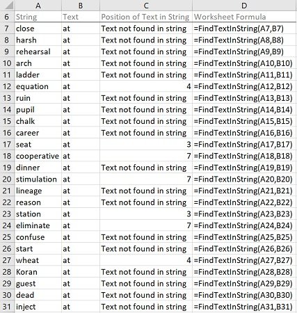
Example: Find text in string with VBA macros

#10. Excel VBA Find Character in String

VBA Code to Find Character in String

To find a character in a string, use the following structure/template in the applicable statement:

InStr(StartingPosition, SearchedString, SearchedCharacter, VbCompareMethodConstant)

The following Sections describe the main elements in this structure.

InStr

The InStr function returns a number. This number specifies the position of the first occurrence of a string or text (SearchedCharacter) in another string (SearchedString).

StartingPosition

The Start argument of the InStr function is:

An optional argument.
A numeric expression specifying the starting position for the character search.

If you omit specifying the Start argument, the search begins at the first character of the searched string (SearchedString).

To find a character in a string, set the Start argument to the position (in SearchedString) where the character search starts.

SearchedString

The String1 argument of the InStr function represents the string expression the InStr function searches in.

To find a character in a string, set the String1 argument to the searched string.

SearchedCharacter

The String2 argument of the InStr function represents the string expression (or text) the InStr function searches for.

To find a character in a string, set the String2 argument to the character you search for.

VbCompareMethodConstant

The Compare argument of the InStr function:

Is an optional argument.
Specifies the type of string comparison carried out by the InStr function.
Can take any of the built-in constants/values from the vbCompareMethod enumeration.

To find a character in a string, set the Compare argument to either of the following, as applicable:

vbBinaryCompare: Performs a binary comparison. vbBinaryCompare:
- Results in a case-sensitive search.
- May be (slightly) faster than vbTextCompare.
vbTextCompare: Performs a textual comparison. vbTextCompare:
- Results in a case-insensitive search.
- May be (slightly) slower than vbBinaryCompare.
- Is more prone to errors/bugs than vbBinaryCompare.

Macro Example to Find Character in String

The following macro (User-Defined Function) example does the following:

Accepts three arguments:
1. MyString: The string you search in.
2. MyCharacter: The character you search for.
3. MyStartingPosition: The starting position for the character search. MyStartingPosition is an optional argument with a default value of 1.
Finds MyCharacter in MyString.
Returns the following:
1. If MyCharacter is not found in MyString, the string “Character not found in string”.
2. If MyCharacter is found in MyString, the position of the first occurrence of MyCharacter in MyString.

Function FindCharacterInString(MyString As Variant, MyCharacter As Variant, Optional MyStartingPosition As Variant = 1) As Variant
    'Source: https://powerspreadsheets.com/
    'For further information: https://powerspreadsheets.com/excel-vba-find/
    
    'This UDF:
        '(1) Accepts three arguments: MyString, MyCharacter and MyStartingPosition (optional argument with a default value of 1)
        '(2) Finds a character passed as argument (MyCharacter) in a string passed as argument (MyString)
        '(3) Returns the following (as applicable):
            'If MyCharacter is not found in MyString: The string "Character not found in string"
            'If MyCharacter is found in MyString: The position of the first occurrence of MyCharacter in MyString
    
    'Obtain position of first occurrence of MyCharacter in MyString
    FindCharacterInString = InStr(MyStartingPosition, MyString, MyCharacter, vbBinaryCompare)
    
    'If MyCharacter is not found in MyString, return the string "Character not found in string"
    If FindCharacterInString = 0 Then FindCharacterInString = "Character not found in string"

End Function

Effects of Executing Macro Example to Find Character in String

The following image illustrates the effects of using the macro (User-Defined Function) example. In this example:

Column A (cells A7 to A31) contains randomly generated words.
Column B (cells B7 to B31) contains a character (a).
Column C (cells C7 to C31) contains worksheet formulas working with the macro (User-Defined Function) example. These worksheet formulas return either of the following (as applicable):
- The string “Character not found in string”, if the character specified in the applicable cell of column B is not found in the string specified in the applicable cell of column A.
- The position of the first occurrence of the character specified in the applicable cell of column B in the string specified in the applicable cell of column A, if the character specified in the applicable cell of column B is found in the string specified in the applicable cell of column A.
Column D (cells D7 to D31) displays the worksheet formulas used in column C (=FindCharacterInString(CellInColumnA,CellInColumnB)).
- The string where the search is carried out is stored in column A (CellInColumnA).
- The searched character is stored in column B (CellInColumnB).

Example: Find character in string with VBA macros

#11. Excel VBA Find Column with Specific Header

VBA Code to Find Column with Specific Header

To find a column with a specific header, use the following structure/template in the applicable statement:

HeaderRowRangeObject.Find(What:=SearchedHeader, After:=SingleCellRangeObject, LookIn:=xlValues, LookAt:=xlWhole, SearchOrder:=xlByColumns, SearchDirection:=XlSearchDirectionConstant, MatchCase:=BooleanValue)

The following Sections describe the main elements in this structure.

HeaderRowRangeObject

A Range object representing the cell range containing the headers you search in.

Find

The Range.Find method:

Finds specific information (the header you search for) in a cell range (HeaderRowRangeObject).
Returns a Range object representing the first cell where the information is found.

What:=SearchedHeader

The What parameter of the Range.Find method specifies the data to search for.

To find a column with a specific header, set the What parameter to the header you search for (SearchedHeader).

After:=SingleCellRangeObject

The After parameter of the Range.Find method specifies the cell after which the search begins. This must be a single cell in the cell range containing the headers you search in (HeaderRowRangeObject).

If you omit specifying the After parameter, the search begins after the first cell of the cell range you search in (HeaderRowRangeObject).

To find a column with a specific header, set the After parameter to a Range object representing the cell after which the search begins.

LookIn:=xlValues

The LookIn parameter of the Range.Find method:

Specifies the type of data to search in.
Can take any of the built-in constants/values from the XlFindLookIn enumeration.

To find a column with a specific header, set the LookIn parameter to xlValues. xlValues refers to values.

LookAt:=xlWhole

The LookAt parameter of the Range.Find method:

Specifies against which of the following the data you are searching for is matched:
- The entire/whole searched cell contents.
- Any part of the searched cell contents.
Can take any of the built-in constants/values from the XlLookAt enumeration.

To find a column with a specific header, set the LookAt parameter to xlWhole. xlWhole matches the data you are searching for against the entire/whole searched cell contents.

SearchOrder:=xlByColumns

The SearchOrder parameter of the Range.Find method:

Specifies the order in which the applicable cell range (HeaderRowRangeObject) is searched:
- By rows.
- By columns.
Can take any of the built-in constants/values from the XlSearchOrder enumeration.

To find a column with a specific header, set the SearchOrder parameter to xlByColumns. xlByColumns searches by columns.

SearchDirection:=XlSearchDirectionConstant

The SearchDirection parameter of the Range.Find method:

Specifies the search direction:
- Search for the previous match.
- Search for the next match.
Can take any of the built-in constants/values from the XlSearchDirection enumeration.

To find a column with a specific header, set the SearchDirection parameter to either of the following, as applicable:

xlNext (SearchDirection:=xlNext): To search for the next match.
xlPrevious (SearchDirection:=xlPrevious): To search for the previous match.

MatchCase:=BooleanValue

The MatchCase parameter of the Range.Find method specifies whether the search is:

Case-sensitive; or
Case-insensitive.

The default value of the MatchCase parameter is False.

To find a column with a specific header, set the MatchCase parameter to either of the following, as applicable:

True (MatchCase:=True): To carry out a case-sensitive search.
False (MatchCase:=False): To carry out a case-insensitive search.

Macro Example to Find Column with Specific Header

The following macro (User-Defined Function) example does the following:

Accepts two arguments:
1. MyRange: The cell range whose first row contains the headers you search in.
2. MyHeader: The header you search for.
Finds MyHeader in the first row of MyRange.
Returns the number of the column containing the first cell in the header row where the header (MyHeader) is found.

Function FindColumnWithSpecificHeader(MyRange As Range, MyHeader As Variant) As Long
    'Source: https://powerspreadsheets.com/
    'For further information: https://powerspreadsheets.com/excel-vba-find/
    
    'This UDF:
        '(1) Accepts 2 arguments: MyRange and MyHeader
        '(2) Finds a header passed as argument (MyHeader) in the first row (the header row) of a cell range passed as argument (MyRange). The search is case-insensitive
        '(3) Returns the number of the column containing the first cell in the header row where the header (MyHeader) is found
    
    With MyRange.Rows(1)
        FindColumnWithSpecificHeader = .Find(What:=MyHeader, After:=.Cells(.Cells.Count), LookIn:=xlValues, LookAt:=xlWhole, SearchOrder:=xlByColumns, SearchDirection:=xlNext, MatchCase:=False).Column
    End With

End Function

Effects of Executing Macro Example to Find Column with Specific Header

The following image illustrates the effects of using the macro (User-Defined Function) example. In this example:

Columns A through H (cells A6 to H31) contain data with the following characteristics:
- Headers in its first row (row 6).
- Randomly generated values.
Cell J7 contains the searched header (Column 3).
Cell K7 contains the worksheet formula that works with the macro (User-Defined Function) example. This worksheet formula returns the column number of the first cell in the header row (cells A6 to H6) of the cell range (MyRange) where the header (MyHeader) is found. This is column 3 (C).
Cell L7 displays the worksheet formula used in cell K7 (=FindColumnWithSpecificHeader(A6:H31,J7)).
- The cell range whose first row contains the headers where the search is carried out contains cells A6 to H31 (A6:H31).
- The searched header is stored in cell J7 (J7).

Example: Find column with specific header with VBA macros

#12. Excel VBA Find Next or Find All

VBA Code to Find Next or Find All

To (i) find the next appearance of specific information or (ii) find all appearances of specific information, use the following structure/template in the applicable procedure:

Dim FoundCell As Range
Dim FirstFoundCellAddress As String
Set FoundCell = SearchedRangeObject.Find(What:=SearchedData, After:=SingleCellRangeObject, LookIn:=XlFindLookInConstant, LookAt:=XlLookAtConstant, SearchOrder:=XlSearchDirectionConstant, SearchDirection:=xlNext, MatchCase:=BooleanValue)
If Not FoundCell Is Nothing Then
    FirstFoundCellAddress = FoundCell.Address
    Do
        Statements
        Set FoundCell = SearchedRangeObject.FindNext(After:=FoundCell)
    Loop Until FoundCell.Address = FirstFoundCellAddress
End If

The following Sections describe the main elements in this structure.

Lines #1 and #2: Dim FoundCell As Range | Dim FirstFoundCellAddress As String

Dim

The Dim statement:

Declares variables.
Allocates storage space.

FoundCell | FirstFoundCellAddress

The names of the variables declared with the Dim statement.

FoundCell holds/represents the cell where the searched data is found.
FirstFoundCellAddress holds/represents the address of the first cell where the searched data is found.

As Range | As String

The data type of the variables declared with the Dim statement.

FoundCell is of the Range object data type. The Range object represents a cell or cell range.
FirstFoundCellAddress is of the String data type. The String data type (generally) holds textual data.

Line #3: Set FoundCell = SearchedRangeObject.Find(What:=SearchedData, After:=SingleCellRangeObject, LookIn:=XlFindLookInConstant, LookAt:=XlLookAtConstant, SearchOrder:=XlSearchDirectionConstant, SearchDirection:=xlNext, MatchCase:=BooleanValue)

Set

The Set statement assigns an object reference to an object variable.

FoundCell

Object variable holding/representing the cell where the searched data is found.

=

The assignment operator assigns an object reference (returned by the Range.Find method) to an object variable (FoundCell).

SearchedRangeObject

A Range object representing the cell range you search in.

Find

The Range.Find method:

Finds specific information (the data you search for) in a cell range (SearchedRangeObject).
Returns a Range object representing the first cell where the information is found.

What:=SearchedData

The What parameter of the Range.Find method specifies the data to search for.

To (i) find the next appearance of specific information or (ii) find all appearances of specific information, set the What parameter to the data you search for (SearchedData).

After:=SingleCellRangeObject

The After parameter of the Range.Find method specifies the cell after which the search begins. This must be a single cell in the cell range you search in (SearchedRangeObject).

If you omit specifying the After parameter, the search begins after the first cell (in the upper left corner) of the cell range you search in (SearchedRangeObject).

To (i) find the next appearance of specific information or (ii) find all appearances of specific information, set the After parameter to a Range object representing the cell after which the search begins.

LookIn:=XlFindLookInConstant

The LookIn parameter of the Range.Find method:

Specifies the type of data to search in.
Can take any of the built-in constants/values from the XlFindLookIn enumeration.

To (i) find the next appearance of specific information or (ii) find all appearances of specific information, set the LookIn parameter to any of the following, as applicable:

xlCommentsThreaded (LookIn:=xlCommentsThreaded): To search in the applicable cell range’s threaded comments.
xlValues (LookIn:=xlValues): To search in the applicable cell range’s values.
xlComments (LookIn:=xlComments): To search in the applicable cell range’s comments/notes.
xlFormulas (LookIn:=xlFormulas): To search in the applicable cell range’s formulas.

LookAt:=XlLookAtConstant

The LookAt parameter of the Range.Find method:

Specifies against which of the following the data you are searching for is matched:
- The entire/whole searched cell contents.
- Any part of the searched cell contents.
Can take any of the built-in constants/values from the XlLookAt enumeration.

To (i) find the next appearance of specific information or (ii) find all appearances of specific information, set the LookAt parameter to either of the following, as applicable:

xlWhole (LookAt:=xlWhole): To match against the entire/whole searched cell contents.
xlPart (LookAt:=xlPart): To match against any part of the searched cell contents.

SearchOrder:=XlSearchDirectionConstant

The SearchOrder parameter of the Range.Find method:

Specifies the order in which the applicable cell range (SearchedRangeObject) is searched:
- By rows.
- By columns.
Can take any of the built-in constants/values from the XlSearchOrder enumeration.

To (i) find the next appearance of specific information or (ii) find all appearances of specific information, set the SearchOrder parameter to either of the following, as applicable:

xlByRows (SearchOrder:=xlByRows): To search by rows.
xlByColumns (SearchOrder:=xlByColumns): To search by columns.

SearchDirection:=xlNext

The SearchDirection parameter of the Range.Find method:

Specifies the search direction:
- Search for the previous match.
- Search for the next match.
Can take any of the built-in constants/values from the XlSearchDirection enumeration.

To (i) find the next appearance of specific information or (ii) find all appearances of specific information, set the SearchDirection parameter to xlNext. xlNext results in the Range.Find method searching for the next match.

MatchCase:=BooleanValue

The MatchCase parameter of the Range.Find method specifies whether the search is:

Case-sensitive; or
Case-insensitive.

The default value of the MatchCase parameter is False.

To (i) find the next appearance of specific information or (ii) find all appearances of specific information, set the MatchCase parameter to either of the following, as applicable:

True (MatchCase:=True): To carry out a case-sensitive search.
False (MatchCase:=False): To carry out a case-insensitive search.

Lines #4 and 10: If Not FoundCell Is Nothing Then | End If

If … Then | End If

The If… Then… Else statement:

Conditionally executes a set of statements (lines #5 to #9);
Depending on an expression’s value (Not FoundCell Is Nothing).

Not FoundCell Is Nothing

The condition of an If… Then… Else statement is an expression evaluating to True or False. If the expression returns True, the applicable set of statements (lines #5 to #9) is executed.

In this expression:

Not FoundCell:
- The Not operator performs a logical negation on an expression.
- FoundCell is the object variable holding/representing the cell where the searched data is found.
- The Range.Find method (in line #3) returns Nothing if no match is found. Therefore:
  - If the Range.Find method finds no match:
    - FoundCell is Nothing.
    - Not FoundCell is not Nothing.
  - If the Range.Find method finds a match:
    - FoundCell is not Nothing.
    - Not FoundCell is Nothing.
Is: The Is operator is an object reference comparison operator.
Nothing: Nothing allows you to disassociate a variable from the data it previously represented. The Range.Find method (in line #3) returns Nothing if no match is found.

Line #5: FirstFoundCellAddress = FoundCell.Address

FirstFoundCellAddress

Variable holding/representing the address of the first cell where the searched data is found.

=

The assignment operator assigns the result returned by an expression (FoundCell.Address) to a variable (FirstFoundCellAddress).

FoundCell

Object variable holding/representing the cell where the searched data is found.

At this point, FoundCell holds/represents the first cell where the searched data is found (by line #3).

Address

The Range.Address property returns a String representing the applicable cell range’s (FoundCell’s) reference.

Lines #6 and #9: Do | Loop Until FoundCell.Address = FirstFoundCellAddress

Do | Loop Until…

The Do… Loop Until statement repeats a set of statements until a condition becomes True.

FoundCell.Address = FirstFoundCellAddress

The condition of a Do… Loop Until statement is an expression evaluating to True or False. The applicable set of statements (lines #7 and #8) are:

(Always) executed once, even if the condition is never met; and
Repeatedly executed until the condition returns True.

In this expression:

FoundCell.Address:
- FoundCell is an object variable holding/representing the cell where the searched data is found.
- The Range.Address property returns a String representing the applicable cell range’s (FoundCell’s) reference.
=: The equal to comparison operator returns True or False as follows:
- True if both expressions (FoundCell.Address and FirstFoundCellAddress) are equal.
- False if the expressions (FoundCell.Address and FirstFoundCellAddress) are not equal.
FirstFoundCellAddress: Variable holding/representing the address of the first cell where the searched data is found.

This condition is tested (only) after the procedure finds (and works with) the first cell where the searched data is found. Therefore, the condition (only) returns True after the Range.FindNext method (line #8) wraps around to the first cell where the searched data is found (after finding all other cells where the searched data is found).

Line #7: Statements

Set of statements to be repeatedly executed for each cell where the searched data is found.

Line #8: Set FoundCell = SearchedRangeObject.FindNext(After:=FoundCell)

Set

The Set statement assigns an object reference to an object variable.

FoundCell

Object variable holding/representing the cell where the searched data is found.

=

The assignment operator assigns an object reference (returned by the Range.FindNext method) to an object variable (FoundCell).

SearchedRangeObject

A Range object representing the cell range you search in.

FindNext

The Range.FindNext method:

Continues the search that was begun by the Range.Find method (line #3).
Finds the next cell matching the conditions specified by the Range.Find method (line #3).
Returns a Range object representing the next cell where the information is found.

After:=FoundCell

The After parameter of the Range.FindNext method specifies the cell after which the search restarts.

To (i) find the next appearance of specific information or (ii) find all appearances of specific information, set the After parameter to the object variable holding/representing the cell where the searched data is found.

Macro Example to Find Next or Find All

The following macro example does the following:

Find:
1. All cells whose value is 10;
2. In the cell range containing cells A6 to H30 in the “Find Next All” worksheet in the workbook where the procedure is stored.
Set the interior/fill color of all found cells to light green.

Sub FindNextAll()
    'Source: https://powerspreadsheets.com/
    'For further information: https://powerspreadsheets.com/excel-vba-find/
    
    'This procedure:
        '(1) Finds all cells whose value is 10 in cells A6 to H30 of the "Find Next All" worksheet in this workbook
        '(2) Sets the found cells' interior/fill color to light green
    
    'Declare variable to hold/represent searched value
    Dim MyValue As Long
    
    'Declare variable to hold/represent address of first cell where searched value is found
    Dim FirstFoundCellAddress As String
    
    'Declare object variable to hold/represent cell range where search takes place
    Dim MyRange As Range
    
    'Declare object variable to hold/represent cell where searched value is found
    Dim FoundCell As Range
    
    'Specify searched value
    MyValue = 10
    
    'Identify cell range where search takes place
    Set MyRange = ThisWorkbook.Worksheets("Find Next All").Range("A6:H30")
    
    'Find first cell where searched value is found
    With MyRange
        Set FoundCell = .Find(What:=MyValue, After:=.Cells(.Cells.Count), LookIn:=xlValues, LookAt:=xlWhole, SearchOrder:=xlByRows, SearchDirection:=xlNext)
    End With
    
    'Test whether searched value is found in cell range where search takes place
    If Not FoundCell Is Nothing Then
        
        'Store address of first cell where searched value is found
        FirstFoundCellAddress = FoundCell.Address
        
        Do
            
            'Set interior/fill color of applicable cell where searched value is found to light green
            FoundCell.Interior.Color = RGB(63, 189, 133)
            
            'Find next cell where searched value is found
            Set FoundCell = MyRange.FindNext(After:=FoundCell)
        
        'Loop until address of current cell where searched value is found is equal to address of first cell where searched value was found
        Loop Until FoundCell.Address = FirstFoundCellAddress
    
    End If
    
End Sub

Effects of Executing Macro Example to Find Next or Find All

The following image illustrates the effects of executing the macro example. In this example:

Cells A6 to H30 contain randomly generated values.
A text box (Find all cells where value = 10) executes the macro example when clicked.

After the macro is executed, Excel sets the interior/fill color of all cells whose value is 10 to light green.

Example: Find next appearance or find all appearances with VBA macros

#13. Excel VBA Find Last Row with Data in Cell Range

VBA Code to Find Last Row with Data in Cell Range

To find the last row with data in a cell range, use the following structure/template in the applicable procedure:

If Application.CountA(SearchedCellRangeObject) = 0 Then
    LastRowVariable = ValueIfCellRangeEmpty
Else
    LastRowVariable = SearchedCellRangeObject.Find(What:="*", LookIn:=xlFormulas, LookAt:=xlPart, SearchOrder:=xlByRows, SearchDirection:=xlPrevious).Row
End If

The following Sections describe the main elements in this structure.

Lines #1, #3 and #5: If Application.CountA(SearchedCellRangeObject) = 0 Then | Else | End If

If… Then … Else… End If

The If… Then… Else statement:

Conditionally executes a set of statements (line #2 or line #4);
Depending on an expression’s value (Application.CountA(SearchedCellRangeObject) = 0).

Application.CountA(SearchedCellRangeObject) = 0

The condition of an If… Then… Else statement is an expression evaluating to True or False.

If the expression returns True, a set of statements (line #2) is executed.
If the expression returns False, a different set of statements (line #4) is executed.

In this expression:

Application.CountA(…): The WorksheetFunction.CountA method counts the number of cells in a cell range (SearchedCellRangeObject) that are not empty.
SearchedCellRangeObject: A Range object representing the cell range whose last row you search.
=: The equal to comparison operator returns True or False as follows:
- True if both expressions (Application.CountA(SearchedCellRangeObject) and 0) are equal.
- False if the expressions (Application.CountA(SearchedCellRangeObject) and 0) are not equal.
0: The number 0. The WorksheetFunction.CountA method returns 0 if all cells in SearchedCellRangeObject are empty.

Line #2: LastRowVariable = ValueIfCellRangeEmpty

Assignment statement assigning:

ValueIfCellRangeEmpty; to
LastRowVariable.

In this expression:

LastRowVariable: Variable of (usually) the Long data type holding/representing the number of the last row with data in the cell range whose last row you search (SearchedCellRangeObject).
=: Assignment operator. Assigns a value (ValueIfCellRangeEmpty) to a variable (LastRowVariable).
ValueIfCellRangeEmpty: Value assigned to LastRowVariable when SearchedCellRangeObject is empty and the WorksheetFunction.CountA method returns 0.

Line #4: LastRowVariable = SearchedCellRangeObject.Find(What:=”*”, LookIn:=xlFormulas, LookAt:=xlPart, SearchOrder:=xlByRows, SearchDirection:=xlPrevious).Row

LastRowVariable

Variable of (usually) the Long data type holding/representing the number of the last row with data in the cell range whose last row you search (SearchedCellRangeObject).

=

The assignment operator assigns a value (SearchedCellRangeObject.Find(What:=”*”, LookIn:=xlFormulas, LookAt:=xlPart, SearchOrder:=xlByRows, SearchDirection:=xlPrevious).Row) to a variable (LastRowVariable).

SearchedCellRangeObject

A Range object representing the cell range whose last row you search.

Find

The Range.Find method:

Finds specific information in a cell range (SearchedCellRangeObject).
Returns a Range object representing the first cell where the information is found.

What:=”*”

The What parameter of the Range.Find method specifies the data to search for.

To find the last row with data in a cell range, set the What parameter to any character sequence. The asterisk (*) acts as a wildcard and results in Range.Find searching for any character sequence.

LookIn:=xlFormulas

The LookIn parameter of the Range.Find method:

Specifies the type of data to search in.
Can take any of the built-in constants/values from the XlFindLookIn enumeration.

To find the last row with data in a cell range, set the LookIn parameter to xlFormulas. xlFormulas refers to formulas.

LookAt:=xlPart

The LookAt parameter of the Range.Find method:

Specifies against which of the following the data you are searching for is matched:
- The entire/whole searched cell contents.
- Any part of the searched cell contents.
Can take any of the built-in constants/values from the XlLookAt enumeration.

To find the last row with data in a cell range, set the LookAt parameter to xlPart. xlPart matches the data you are searching for (any character sequence as specified by the What parameter) against any part of the searched cell contents.

SearchOrder:=xlByRows

The SearchOrder parameter of the Range.Find method:

Specifies the order in which the applicable cell range (SearchedCellRangeObject) is searched:
- By rows.
- By columns.
Can take any of the built-in constants/values from the XlSearchOrder enumeration.

To find the last row with data in a cell range, set the SearchOrder parameter to xlByRows. xlByRows results in the Range.Find method searching by rows.

SearchDirection:=xlPrevious

The SearchDirection parameter of the Range.Find method:

Specifies the search direction:
- Search for the previous match.
- Search for the next match.
Can take any of the built-in constants/values from the XlSearchDirection enumeration.

To find the last row with data in a cell range, set the SearchDirection parameter to xlPrevious. xlPrevious results in the Range.Find method searching for the previous match.

Row

The Range.Row property returns the number of the first row of the first area in a cell range.

When searching for the last row with data in a cell range, the Range.Row property returns the row number of the cell represented by the Range object returned by the Range.Find method (Find(What:=”*”, LookIn:=xlFormulas, LookAt:=xlPart, SearchOrder:=xlByRows, SearchDirection:=xlPrevious)).

Macro Example to Find Last Row with Data in Cell Range

The following macro (User-Defined Function) example does the following:

Accepts one argument (MyRange). This is the cell range whose last row you search.
Tests whether MyRange is empty and proceeds accordingly:
1. If MyRange is empty, returns the number 0 as the number of the last row with data in MyRange.
2. If MyRange isn’t empty:
  1. Finds the last row with data in MyRange; and
  2. Returns the number of the last row with data in MyRange.

Function FindLastRow(MyRange As Range) As Long
    'Source: https://powerspreadsheets.com/
    'For further information: https://powerspreadsheets.com/excel-vba-find/
    
    'This UDF:
        '(1) Accepts 1 argument: MyRange
        '(2) Tests whether MyRange is empty
        '(3) If MyRange is empty, returns 0 as the number of the last row with data in MyRange
        '(4) If MyRange is not empty:
            '(1) Finds the last row with data in MyRange by searching for the last cell with any character sequence
            '(2) Returns the number of the last row with data in MyRange
        
    'Test if MyRange is empty
    If Application.CountA(MyRange) = 0 Then

        'If MyRange is empty, assign 0 to FindLastRow
        FindLastRow = 0

    Else
    
        'If MyRange isn't empty, find the last cell with any character sequence by:
            '(1) Searching for the previous match;
            '(2) Across rows
        FindLastRow = MyRange.Find(What:="*", LookIn:=xlFormulas, LookAt:=xlPart, SearchOrder:=xlByRows, SearchDirection:=xlPrevious).Row

    End If
    
End Function

Effects of Executing Macro Example to Find Last Row with Data in Cell Range

The following image illustrates the effects of using the macro (User-Defined Function) example. In this example:

Columns A through H (cells A6 to H30) contain data.
Cell J7 contains the worksheet formula that works with the macro (User-Defined Function) example. This worksheet formula returns the number of the last row with data in the cell range (MyRange). This is row 30.
Cell K7 displays the worksheet formula used in cell J7 (=FindLastRow(A:H)). The cell range whose last row is searched contains columns A through H (A:H).

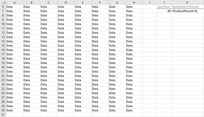
#14. Excel VBA Find Last Column with Data in Cell Range

VBA Code to Find Last Column with Data in Cell Range

To find the last column with data in a cell range, use the following structure/template in the applicable procedure:

If Application.CountA(SearchedCellRangeObject) = 0 Then
    LastColumnVariable = ValueIfCellRangeEmpty
Else
    LastColumnVariable = SearchedCellRangeObject.Find(What:="*", LookIn:=xlFormulas, LookAt:=xlPart, SearchOrder:=xlByColumns, SearchDirection:=xlPrevious).Column
End If

The following Sections describe the main elements in this structure.

Lines #1, #3 and #5: If Application.CountA(SearchedCellRangeObject) = 0 Then | Else | End If

If… Then … Else… End If

The If… Then… Else statement:

Conditionally executes a set of statements (line #2 or line #4);
Depending on an expression’s value (Application.CountA(SearchedCellRangeObject) = 0).

Application.CountA(SearchedCellRangeObject) = 0

The condition of an If… Then… Else statement is an expression evaluating to True or False.

If the expression returns True, a set of statements (line #2) is executed.
If the expression returns False, a different set of statements (line #4) is executed.

In this expression:

Application.CountA(…): The WorksheetFunction.CountA method counts the number of cells in a cell range (SearchedCellRangeObject) that are not empty.
SearchedCellRangeObject: A Range object representing the cell range whose last column you search.
=: The equal to comparison operator returns True or False as follows:
- True if both expressions (Application.CountA(SearchedCellRangeObject) and 0) are equal.
- False if the expressions (Application.CountA(SearchedCellRangeObject) and 0) are not equal.
0: The number 0. The WorksheetFunction.CountA method returns 0 if all cells in SearchedCellRangeObject are empty.

Line #2: LastColumnVariable = ValueIfCellRangeEmpty

Assignment statement assigning:

ValueIfCellRangeEmpty; to
LastColumnVariable.

In this expression:

LastColumnVariable: Variable of (usually) the Long data type holding/representing the number of the last column with data in the cell range whose last column you search (SearchedCellRangeObject).
=: Assignment operator. Assigns a value (ValueIfCellRangeEmpty) to a variable (LastColumnVariable).
ValueIfCellRangeEmpty: Value assigned to LastColumnVariable when SearchedCellRangeObject is empty and the WorksheetFunction.CountA method returns 0.

Line #4: LastColumnVariable = SearchedCellRangeObject.Find(What:=”*”, LookIn:=xlFormulas, LookAt:=xlPart, SearchOrder:=xlByColumns, SearchDirection:=xlPrevious).Column

LastColumnVariable

Variable of (usually) the Long data type holding/representing the number of the last column with data in the cell range whose last column you search (SearchedCellRangeObject).

=

The assignment operator assigns a value (SearchedCellRangeObject.Find(What:=”*”, LookIn:=xlFormulas, LookAt:=xlPart, SearchOrder:=xlByColumns, SearchDirection:=xlPrevious).Column) to a variable (LastColumnVariable).

SearchedCellRangeObject

A Range object representing the cell range whose last column you search.

Find

The Range.Find method:

Finds specific information in a cell range (SearchedCellRangeObject).
Returns a Range object representing the first cell where the information is found.

What:=”*”

The What parameter of the Range.Find method specifies the data to search for.

To find the last column with data in a cell range, set the What parameter to any character sequence. The asterisk (*) acts as a wildcard and results in Range.Find searching for any character sequence.

LookIn:=xlFormulas

The LookIn parameter of the Range.Find method:

Specifies the type of data to search in.
Can take any of the built-in constants/values from the XlFindLookIn enumeration.

To find the last column with data in a cell range, set the LookIn parameter to xlFormulas. xlFormulas refers to formulas.

LookAt:=xlPart

The LookAt parameter of the Range.Find method:

Specifies against which of the following the data you are searching for is matched:
- The entire/whole searched cell contents.
- Any part of the searched cell contents.
Can take any of the built-in constants/values from the XlLookAt enumeration.

To find the last column with data in a cell range, set the LookAt parameter to xlPart. xlPart matches the data you are searching for (any character sequence as specified by the What parameter) against any part of the searched cell contents.

SearchOrder:=xlByColumns

The SearchOrder parameter of the Range.Find method:

Specifies the order in which the applicable cell range (SearchedCellRangeObject) is searched:
- By rows.
- By columns.
Can take any of the built-in constants/values from the XlSearchOrder enumeration.

To find the last column with data in a cell range, set the SearchOrder parameter to xlByColumns. xlByColumns results in the Range.Find method searching by columns.

SearchDirection:=xlPrevious

The SearchDirection parameter of the Range.Find method:

Specifies the search direction:
- Search for the previous match.
- Search for the next match.
Can take any of the built-in constants/values from the XlSearchDirection enumeration.

To find the last column with data in a cell range, set the SearchDirection parameter to xlPrevious. xlPrevious results in the Range.Find method searching for the previous match.

Column

The Range.Column property returns the number of the first column of the first area in a cell range.

When searching for the last column with data in a cell range, the Range.Column property returns the column number of the cell represented by the Range object returned by the Range.Find method (Find(What:=”*”, LookIn:=xlFormulas, LookAt:=xlPart, SearchOrder:=xlByColumns, SearchDirection:=xlPrevious)).

Macro Example to Find Last Column with Data in Cell Range

The following macro (User-Defined Function) example does the following:

Accepts one argument (MyWorksheetName). This is the name of the worksheet whose last column you search.
Tests whether the worksheet named MyWorksheetName is empty and proceeds accordingly:
1. If the worksheet named MyWorksheetName is empty, returns the number 0 as the number of the last column with data in the worksheet.
2. If the worksheet named MyWorksheetName isn’t empty:
  1. Finds the last column with data in the worksheet; and
  2. Returns the number of the last column with data in the worksheet.

Function FindLastColumn(MyWorksheetName As String) As Long
    'Source: https://powerspreadsheets.com/
    'For further information: https://powerspreadsheets.com/excel-vba-find/
    
    'This UDF:
        '(1) Accepts 1 argument: MyWorksheetName
        '(2) Tests whether the worksheet named MyWorksheetName is empty
        '(3) If the worksheet named MyWorksheetName is empty, returns 0 as the number of the last column with data in the worksheet
        '(4) If the worksheet named MyWorksheetName is not empty:
            '(1) Finds the last column with data in the worksheet by searching for the last cell with any character sequence
            '(2) Returns the number of the last column with data in the worksheet
    
    'Declare object variable to hold/represent all cells in the worksheet named MyWorksheetName
    Dim MyRange As Range
    
    'Identify all cells in the worksheet named MyWorksheetName
    Set MyRange = ThisWorkbook.Worksheets(MyWorksheetName).Cells
    
    'Test if MyRange is empty
    If Application.CountA(MyRange) = 0 Then

        'If MyRange is empty, assign 0 to FindLastColumn
        FindLastColumn = 0

    Else
    
        'If MyRange isn't empty, find the last cell with any character sequence by:
            '(1) Searching for the previous match;
            '(2) Across columns
        FindLastColumn = MyRange.Find(What:="*", LookIn:=xlFormulas, LookAt:=xlPart, SearchOrder:=xlByColumns, SearchDirection:=xlPrevious).Column

    End If
    
End Function

Effects of Executing Macro Example to Find Last Column with Data in Cell Range

The following image illustrates the effects of using the macro (User-Defined Function) example. In this example:

Columns A through H (cells A6 to H30) in the worksheet named “Find Last Column Data” contain data.
- Columns A through H of the “Find Last Column Data” worksheet contain exactly the same data as that in the “Find Last Column Formula” worksheet (displayed in the image below).
- The “Find Last Column Data” worksheet contains no data in columns J or K whereas the “Find Last Column Formula” worksheet (displayed in the image below) does.
Cell J7 contains the worksheet formula that works with the macro (User-Defined Function) example. This worksheet formula returns the number of the last column with data in the worksheet (named “Find Last Column Data”). This is column H or 8.
Cell K7 displays the worksheet formula used in cell J7 (=FindLastColumn(“Find Last Column Data”)). The name of the worksheet whose last column is searched is “Find Last Column Data”.

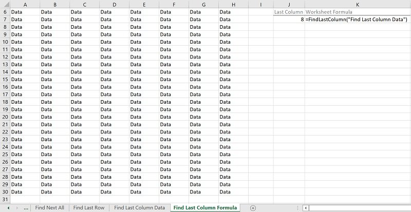
#15. Excel VBA Find Last Non Empty Cell in Column

VBA Code to Find Last Non Empty Cell in Column

To find the last non empty cell in a column, use the following structure/template in the applicable statement:

WorksheetObject.Range(ColumnLetter & WorksheetObject.Rows.Count).End(xlUp)

The following Sections describe the main elements in this structure.

WorksheetObject

A Worksheet object representing the worksheet containing the column whose last non empty cell you want to find.

Range

The Worksheet.Range property returns a Range object representing a cell or cell range.

ColumnLetter

The letter of the column whose last non empty cell you want to find.

&

The concatenation operator joins two strings and creates a new string.

WorksheetObject

A Worksheet object representing the worksheet containing the column whose last non empty cell you want to find.

Rows

The Worksheet.Rows property returns a Range object representing all rows in the applicable worksheet (containing the column whose last non empty cell you want to find).

Count

The Range.Count property returns the number of objects in a collection (the number of rows in the worksheet containing the column whose last non empty cell you want to find).

End(xlUp)

The Range.End property returns a Range object representing the cell at the end of the region containing the source range. In other words: The Range.End property is the rough equivalent of using the “Ctrl + Arrow Key” or “End, Arrow Key” keyboard shortcuts.

The Range.End property accepts one parameter: Direction. Direction:

Specifies the direction in which to move.
Can take the any of the built-in constants/values from the XlDirection enumeration.

To find the last non empty cell in a column, set the Direction parameter to xlUp. xlUp:

Results in moving up, to the top of the data region.
Is the rough equivalent of the “Ctrl + Up Arrow” or “End, Up Arrow” keyboard shortcuts.

Macro Example to Find Last Non Empty Cell in Column

The following macro (User-Defined Function) example does the following:

Accepts one argument (MyColumn): The letter of the column (in the worksheet where the UDF is used) whose last non empty cell you want to find.
Finds the last non empty cell in the applicable column.
Returns a string containing the address (as an A1-style relative reference) of the last non empty cell in the applicable column.

Function FindLastNonEmptyCellColumn(MyColumn As String) As String
    'Source: https://powerspreadsheets.com/
    'For further information: https://powerspreadsheets.com/excel-vba-find/
    
    'This UDF:
        '(1) Accepts 1 argument: MyColumn
        '(2) Finds the last non empty cell in the column whose letter is passed as argument (MyColumn) in the worksheet where the UDF is used
        '(3) Returns the address (as an A1-style relative reference) of the last non empty cell found in the column whose letter is passed as argument (MyColumn) in the worksheet where the UDF is used
    With Application.Caller.Parent
        FindLastNonEmptyCellColumn = .Range(MyColumn & .Rows.Count).End(xlUp).Address(RowAbsolute:=False, ColumnAbsolute:=False)
    End With

End Function

Effects of Executing Macro Example to Find Last Non Empty Cell in Column

The following image illustrates the effects of using the macro (User-Defined Function) example. In this example:

Column A (cells A6 to A30) contains data.
Cell C7 contains the letter of the column whose last non empty cell is sought (A).
Cell D7 contains the worksheet formula that works with the macro (User-Defined Function) example. This worksheet formula returns the address (as an A1-style relative reference) of the last non empty cell in column A (MyColumn). This is cell A30
Cell E7 displays the worksheet formula used in cell D7 (=FindLastNonEmptyCellColumn(C7)). The letter of the column whose last non empty cell is sought is stored in cell C7 (C7).

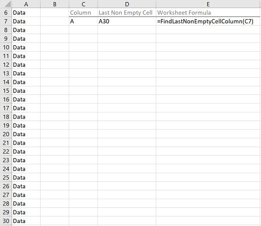
Example: Find last non empty cell in column with VBA macros

#16. Excel VBA Find Empty (or Blank) Cells

VBA Code to Find Empty (or Blank) Cells

To find all empty (or blank) cells in a cell range, use the following structure/template in the applicable procedure:

Dim BlankCellsObjectVariable As Range
On Error Resume Next
Set BlankCellsObjectVariable = RangeObjectWithBlankCells.SpecialCells(xlCellTypeBlanks)
On Error GoTo 0
If Not BlankCellsObjectVariable Is Nothing Then
    StatementsIfBlankCells
End If

The following Sections describe the main elements in this structure.

Line #1: Dim BlankCellsObjectVariable As Range

Dim

The Dim statement:

Declares variables.
Allocates storage space.

BlankCellsObjectVariable

The name of the variable declared with the Dim statement.

BlankCellsObjectVariable holds/represents the empty (or blank) cells found.

As Range

The data type of the variable declared with the Dim statement.

BlankCellsObjectVariable is declared as of the Range object data type. The Range object represents a cell or cell range.

Line #2: On Error Resume Next

The On Error Resume Next statement specifies that, when a run-time error occurs, control passes to the statement immediately following that statement where the error occurred. Therefore, procedure execution continues.

Line #3 returns an error (Run time error ‘1004′: No cells were found) if the cell range where you search for empty (or blank) cells doesn’t contain any empty (or blank) cells.

Line #3: Set BlankCellsObjectVariable = RangeObjectWithBlankCells.SpecialCells(xlCellTypeBlanks)

Set

The Set statement assigns an object reference to an object variable.

BlankCellsObjectVariable

Object variable holding/representing the empty (or blank) cells found.

=

The assignment operator assigns an object reference (returned by the Range.SpecialCells method) to an object variable (BlankCellsObjectVariable).

RangeObjectWithBlankCells

A Range object representing the cell range you search in for empty (or blank) cells.

SpecialCells

The Range.SpecialCells method returns a Range object representing all cells matching a specified:

Type; and
Value.

xlCellTypeBlanks

The Type parameter of the Range.SpecialCells method:

Specifies the cells to include in the Range object returned by the Range.SpecialCells method.
Can take any of the built-in constants/values from the XlCellType enumeration.

To find all empty (or blank) cells in a cell range, set the Type parameter to xlCellTypeBlanks. xlCellTypeBlanks results in the Range.SpecialCells method including blank/empty cells in the Range object it returns.

Line #4: On Error GoTo 0

The On Error GoTo 0 statement disables error handling (originally enabled by line #2).

Line #5 and #7: If Not BlankCellsObjectVariable Is Nothing Then | End If

If… Then | End If

The If… Then… Else statement:

Conditionally executes a set of statements (line #6);
Depending on an expression’s value (Not BlankCellsObjectVariable Is Nothing).

Not BlankCellsObjectVariable Is Nothing

The condition of an If… Then… Else statement is an expression evaluating to True or False. If the expression returns True, the applicable set of statements (line #6) is executed.

In this expression:

Not BlankCellsObjectVariable:
- The Not operator performs a logical negation on an expression.
- BlankCellsObjectVariable is the object variable holding/representing the empty (or blank) cells found.
- BlankCellsObjectVariable holds/represents Nothing if no empty (or blank) cells are found. Therefore:
  - If the Range.SpecialCells method finds no empty (or blank) cells:
    - BlankCellsObjectVariable is Nothing.
    - Not BlankCellsObjectVariable is not Nothing.
  - If the Range.SpecialCells method finds empty (or blank) cells:
    - BlankCellsObjectVariable is not Nothing.
    - Not BlankCellsObjectVariable is Nothing.
Is: The Is operator is an object reference comparison operator.
Nothing: Nothing allows you to disassociate a variable from the data it previously represented. BlankCellsObjectVariable holds/represents Nothing if no empty (or blank) cells are found.

Line #6: StatementsIfBlankCells

Statements conditionally executed by the If… Then… Else statement if the applicable condition (Not BlankCellsObjectVariable Is Nothing) returns True (the Range.SpecialCells method finds empty or blank cells).

Macro Example to Find Empty (or Blank) Cells

The following macro example does the following:

Find all empty (or blank) cells in the cell range containing cells A6 to H30 in the “Find Blank Cells” worksheet in the workbook where the procedure is stored.
Set the interior/fill color of all found empty (or blank) cells to light green.

Sub FindBlankCells()
    'Source: https://powerspreadsheets.com/
    'For further information: https://powerspreadsheets.com/excel-vba-find/
    
    'This procedure:
        '(1) Finds all blank cells in cells A6 to H30 of the "Find Blank Cells" worksheet in this workbook
        '(2) Sets the found cells' interior/fill color to light green
    
    'Declare object variable to hold/represent blank cells
    Dim MyBlankCells As Range
        
    'Enable error-handling
    On Error Resume Next
    
    'Identify blank cells in searched cell range
    Set MyBlankCells = ThisWorkbook.Worksheets("Find Blank Cells").Range("A6:H30").SpecialCells(xlCellTypeBlanks)
    
    'Disable error-handling
    On Error GoTo 0
    
    'Test whether blank cells were found in searched cell range
    If Not MyBlankCells Is Nothing Then
        
        'Set interior/fill color of blank cells found to light green
        MyBlankCells.Interior.Color = RGB(63, 189, 133)
        
    End If

End Sub

Effects of Executing Macro Example to Find Empty (or Blank) Cells

The following image illustrates the effects of using the macro example. In this example:

Columns A through H (cells A6 to H30) contain:
- Data; and
- A few empty cells (with light green interior/fill).
A text box (Find all blank cells) executes the macro example when clicked.

After the macro is executed, Excel sets the interior/fill color of all empty (or blank) cells to light green.

Example: Find blank cells with VBA macros

#17. Excel VBA Find First Empty (or Blank) Cell in Cell Range

VBA Code to Find First Empty (or Blank) Cell in Cell Range

To find the first empty (or blank) cell in a cell range, use the following structure/template in the applicable procedure:

For Each iCell In CellRangeObject
    If IsEmpty(iCell) Then
        StatementsForFirstEmptyCell
        Exit For
    End If
Next iCell

The following Sections describe the main elements in this structure.

Lines #1 and #6: For Each iCell In CellRangeObject | Next iCell

For Each … In … | Next …

The For Each… Next statement repeats a series of statements for each element (iCell, an individual cell) in a collection (CellRangeObject).

iCell

Object variable (of the Range data type) used to iterate/loop through each element of the collection (CellRangeObject).

CellRangeObject

A Range object representing the cell range you search in.

The series of statements repeated by the For Each… Next statement are repeated for each individual element (iCell) in CellRangeObject.

Lines #2 and #5: If IsEmpty(iCell) Then | End If

If… Then | End If

The If… Then Else statement:

Conditionally executes a set of statements (lines #3 and #4);
Depending on an expression’s value (IsEmpty(iCell)).

IsEmpty(iCell)

The condition of an If… Then… Else statement is an expression evaluating to True or False. If the expression returns True, the applicable set of statements (lines #3 and #4) are executed.

In this expression:

As a general rule, the IsEmpty function returns a Boolean value (True or False) indicating whether a variable is initialized. You can (also) use the IsEmpty function to test whether a cell is empty (or blank).
iCell is an object variable representing the individual cell the For Each… Next statement is currently working with (iterating through).
IsEmpty(iCell) returns True or False as follows:
- True if the cell (currently) represented by iCell is empty (or blank).
- False if the cell (currently) represented by iCell isn’t empty. A cell isn’t considered to be empty if, for example, it contains a worksheet formula returning a zero-length string (“”).

Line #3: StatementsForFirstEmptyCell

Statements conditionally executed by the If… Then… Else statement if the applicable condition (IsEmpty(iCell)) returns True (the cell currently represented by iCell is empty or blank).

Line #4: Exit For

The Exit For statement:

Exits a For Each… Next loop.
Transfers control to the statement following the Next statement (line #6).

Macro Example to Find First Empty (or Blank) Cell in Cell Range

The following macro (User-Defined Function) example does the following:

Accepts one argument (MyRange): The cell range whose first empty cell you search for.
Loops through each individual cell in the cell range (MyRange) and tests whether the applicable cell is empty (or blank).
Returns the following:
1. If MyRange contains empty cells, the address (as an A1-style relative reference) of the first empty cell in the cell range (MyRange).
2. If MyRange doesn’t contain empty cells, the string “No empty cells found in cell range”.

Function FindNextEmptyCellRange(MyRange As Range) As String
    'Source: https://powerspreadsheets.com/
    'For further information: https://powerspreadsheets.com/excel-vba-find/
    
    'This UDF:
        '(1) Accepts 1 argument: MyRange
        '(2) Loops through each individual cell in the cell range (MyRange) and tests whether the applicable cell is empty
        '(3) Returns the following (as applicable):
            'If there are empty cells in MyRange: The address (as an A1-style relative reference) of the first empty cell
            'If there are no empty cells in MyRange: The string "No empty cells found in cell range"
    
    'Declare object variable to iterate/loop through all cells in the cell range (MyRange)
    Dim iCell As Range
    
    'Loop through each cell in the cell range (MyRange)
    For Each iCell In MyRange
        
        'If the current cell is empty:
            '(1) Return the current cell's address (as an A1-style relative reference)
            '(2) Exit the For Each... Next loop
        If IsEmpty(iCell) Then
            FindNextEmptyCellRange = iCell.Address(RowAbsolute:=False, ColumnAbsolute:=False)
            Exit For
        End If
        
    Next iCell
    
    'If no empty cells are found in the cell range (MyRange), return the string "No empty cells found in cell range"
    If FindNextEmptyCellRange = "" Then FindNextEmptyCellRange = "No empty cells found in cell range"

End Function

Effects of Executing Macro Example to Find First Empty (or Blank) Cell in Cell Range

The following image illustrates the effects of using the macro (User-Defined Function) example. In this example:

Columns A through H (cells A6 to H30) contain:
- Data; and
- A few empty cells (with light green interior/fill).
Cell J7 contains the worksheet formula that works with the macro (User-Defined Function) example. This worksheet formula returns the address (as an A1-style relative reference) of the first empty cell in the cell range (MyRange). This is cell B7.
Cell K7 displays the worksheet formula used in cell J7 (=FindNextEmptyCellRange(A6:H30)). The cell range where the search is carried out contains cells A6 to H30 (A6:H30).

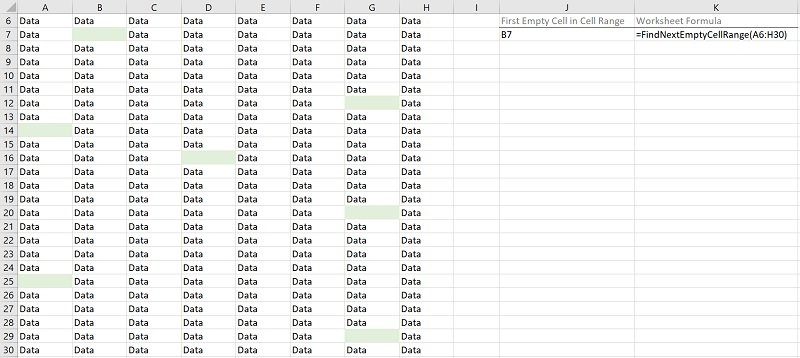
Example: Find first empty cell in cell range with VBA macros

#18. Excel VBA Find First Empty (or Blank) Cell in Column

VBA Code to Find First Empty (or Blank) Cell in Column

To find the first empty (or blank) cell in a column, use the following structure/template in the applicable statement:

ColumnRangeObject.Find(What:="", After:=ColumnRangeObject.Cells(ColumnRangeObject.Cells.Count), LookIn:=xlFormulas, LookAt:=xlWhole, SearchOrder:=xlByRows, SearchDirection:=xlNext)

The following Sections describe the main elements in this structure.

ColumnRangeObject

A Range object representing the column whose first empty (or blank) cell you search for.

Find

The Range.Find method:

Finds specific information (the first empty or blank cell) in a cell range (ColumnRangeObject).
Returns a Range object representing the first cell where the information is found.

What:=””

The What parameter of the Range.Find method specifies the data to search for.

To find the first empty (or blank) cell in a column, set the What parameter to a zero-length string (“”).

After:=ColumnRangeObject.Cells(ColumnRangeObject.Cells.Count)

The After parameter of the Range.Find method specifies the cell after which the search begins.

To find the first empty (or blank) cell in a column, set the After parameter to “ColumnRangeObject.Cells(ColumnRangeObject.Cells.Count)”. For these purposes:

“ColumnRangeObject” is a Range object representing the column whose first empty (or blank) cell you search for.
The Range.Cells property (Cells) returns a Range object representing all cells in the column whose first empty (or blank) cell you search for.
The Range.Item property returns a Range object representing the last cell in the column whose first empty (or blank) cell you search for. For these purposes, the RowIndex parameter of the Range.Item property is set to the value returned by the Range.Count property (Count).
The Range.Count property (Count) returns the number of cells in the Range object returned by the Range.Cells property (ColumnRangeObject.Cells).

LookIn:=xlFormulas

The LookIn parameter of the Range.Find method:

Specifies the type of data to search in.
Can take any of the built-in constants/values from the XlFindLookIn enumeration.

To find the first empty (or blank) cell in a column, set the LookIn parameter to xlFormulas. xlFormulas refers to formulas.

LookAt:=xlWhole

The LookAt parameter of the Range.Find method:

Specifies against which of the following the data you are searching for is matched:
- The entire/whole searched cell contents.
- Any part of the searched cell contents.
The LookAt parameter can take any of the built-in constants/values from the XlLookAt enumeration.

To find the first empty (or blank) cell in a column, set the LookAt parameter to xlWhole. xlWhole matches the data you are searching for against the entire/whole searched cell contents.

SearchOrder:=xlByRows

The SearchOrder parameter of the Range.Find method:

Specifies the order in which the applicable cell range (ColumnRangeObject) is searched:
- By rows.
- By columns.
Can take any of the built-in constants/values from the XlSearchOrder enumeration.

To find the first empty (or blank) cell in a column, set the SearchOrder parameter to xlByRows. xlByRows searches by rows.

SearchDirection:=xlNext

The SearchDirection parameter of the Range.Find method:

Specifies the search direction:
- Search for the previous match.
- Search for the next match.
Can take any of the built-in constants/values from the XlSearchDirection enumeration.

To find the first empty (or blank) cell in a column, set the SearchDirection parameter to xlNext. xlNext searches for the next match.

Macro Example to Find First Empty (or Blank) Cell in Column

The following macro (User-Defined Function) example does the following:

Accepts one argument (MyColumn): The letter of the column (in the worksheet where the UDF is used) whose first empty (or blank) cell you search for.
Finds the first empty (or blank) cell in the applicable column.
Returns a string containing the address (as an A1-style relative reference) of the first empty (or blank) cell in the applicable column.

Function FindFirstEmptyCellColumn(MyColumn As String) As String
    'Source: https://powerspreadsheets.com/
    'For further information: https://powerspreadsheets.com/excel-vba-find/
    
    'This UDF:
        '(1) Accepts 1 argument: MyColumn
        '(2) Finds the first empty (blank) cell in the column whose letter is passed as argument (MyColumn) in the worksheet where the UDF is used
        '(3) Returns the address (as an A1-style relative reference) of the first empty (blank) cell in the column whose letter is passed as argument (MyColumn) in the worksheet where the UDF is used
    With Application.Caller.Parent.Columns(MyColumn)
        FindFirstEmptyCellColumn = .Find(What:="", After:=.Cells(.Cells.Count), LookIn:=xlFormulas, LookAt:=xlWhole, SearchOrder:=xlByRows, SearchDirection:=xlNext).Address(RowAbsolute:=False, ColumnAbsolute:=False)
    End With

End Function

Effects of Executing Macro Example to Find First Empty (or Blank) Cell in Column

The following image illustrates the effects of using the macro (User-Defined Function) example. In this example:

Column I (cells I1 to I25) contains:
- Data; and
- A few empty cells (with light green interior/fill).
Cell A7 contains the letter of the column whose first empty (or blank) cell is sought (I).
Cell B7 contains the worksheet formula that works with the macro (User-Defined Function) example. This worksheet formula returns the address (as an A1-style relative reference) of the first empty (or blank) cell in column I (MyColumn). This is cell I10.
Cell C7 displays the worksheet formula used in cell B7 (=FindFirstEmptyCellColumn(A7)). The letter of the column whose first empty (or blank) cell is sought is stored in cell A7 (A7).

#19. Excel VBA Find Next Empty (or Blank) Cell in Column

VBA Code to Find Next Empty (or Blank) Cell in Column

To find the next empty (or blank) cell in a column, use the following structure/template in the applicable procedure:

If IsEmpty(RangeObjectSourceCell) Then
    RangeObjectSourceCell.ActionForNextEmptyCell
ElseIf IsEmpty(RangeObjectSourceCell.Offset(1, 0)) Then
    RangeObjectSourceCell.Offset(1, 0).ActionForNextEmptyCell
Else
    RangeObjectSourceCell.End(xlDown).Offset(1, 0).ActionForNextEmptyCell
End If

The following Sections describe the main elements in this structure.

Lines #1, #3, #5 and #7: If IsEmpty(RangeObjectSourceCell) Then | ElseIf IsEmpty(RangeObjectSourceCell.Offset(1, 0)) Then | Else | End If

If… Then | ElseIf… Then | Else | End If

The If… Then… Else statement:

Conditionally executes a set of statements (lines #2, #4 or #6);
Depending on an expression’s value (IsEmpty(RangeObjectSourceCell) or IsEmpty(RangeObjectSourceCell.Offset(1, 0))).

IsEmpty(RangeObjectSourceCell)

The condition of an If… Then… Else statement is an expression evaluating to True or False. If the expression returns True, the applicable set of statements (line #2) is executed.

In this expression:

As a general rule, the IsEmpty function returns a Boolean value (True or False) indicating whether a variable is initialized. You can (also) use the IsEmpty function to test whether a cell is empty (or blank).
RangeObjectSourceCell is a Range object representing the cell where the search (for the next empty or blank cell in the column) begins.
IsEmpty(RangeObjectSourceCell) returns True or False as follows:
- True if the cell represented by RangeObjectSourceCell is empty (or blank).
- False if the cell represented by RangeObjectSourceCell isn’t empty. A cell isn’t considered to be empty if, for example, it contains a worksheet formula returning a zero-length string (“”).

IsEmpty(RangeObjectSourceCell.Offset(1, 0))

The condition of an If… Then… Else statement is an expression evaluating to True or False. If the expression returns True, the applicable set of statements (line #4) is executed.

In this expression:

As a general rule, the IsEmpty function returns a Boolean value (True or False) indicating whether a variable is initialized. You can (also) use the IsEmpty function to test whether a cell is empty (or blank).
RangeObjectSourceCell is a Range object representing the cell where the search (for the next empty or blank cell in the column) begins.
The Range.Offset property (Offset(1, 0)) returns a Range object representing a cell range at an offset from the source cell range. In this expression:
- The source cell range is the cell where the search (for the next empty or blank cell in the column) begins (RangeObjectSourceCell).
- The offset from the source cell range is as follows:
  - 1 row downwards, as specified by the RowOffset parameter of the Range.Offset property (1).
  - No column offsetting, as specified by the ColumnOffset parameter of the Range.Offset property (0).
IsEmpty(RangeObjectSourceCell.Offset(1, 0)) returns True or False as follows:
- True if the cell represented by the Range object returned by the Range.Offset property is empty.
- False if the cell represented by the Range object returned by the Range.Offset property isn’t empty. A cell isn’t considered to be empty if, for example, it contains a worksheet formula returning a zero-length string (“”).

Line #2: RangeObjectSourceCell.ActionForNextEmptyCell

Statement conditionally executed by the If… Then… Else statement if the applicable condition (IsEmpty(RangeObjectSourceCell)) returns True.

RangeObjectSourceCell

A Range object representing the cell where the search (for the next empty or blank cell in the column) begins.

ActionForNextEmptyCell

VBA construct (usually a property or method) working with the applicable cell (represented by RangeObjectSourceCell).

Line #4: RangeObjectSourceCell.Offset(1, 0).ActionForNextEmptyCell

Statement conditionally executed by the If… Then… Else statement if the applicable condition (IsEmpty(RangeObjectSourceCell.Offset(1, 0))) returns True.

RangeObjectSourceCell

A Range object representing the cell where the search (for the next empty or blank cell in the column) begins.

Offset(1, 0)

The Range.Offset property (Offset(1, 0)) returns a Range object representing a cell range at an offset from the source cell range. For these purposes:

The source cell range is the cell where the search (for the next empty or blank cell in the column) begins (RangeObjectSourceCell).
The offset from the source cell range is as follows:
- 1 row downwards, as specified by the RowOffset parameter of the Range.Offset property (1).
- No column offsetting, as specified by the ColumnOffset parameter of the Range.Offset property (0).

ActionForNextEmptyCell

VBA construct (usually a property or method) working with the applicable cell (returned by the Range.Offset property).

Line #6: RangeObjectSourceCell.End(xlDown).Offset(1, 0).ActionForNextEmptyCell

Statement conditionally executed by the If… Then… Else statement if no previous condition (in lines #1 or #3) returns True.

RangeObjectSourceCell

A Range object representing the cell where the search (for the next empty or blank cell in the column) begins.

End(xlDown)

The Range.End property accepts one parameter: Direction. Direction:

Specifies the direction in which to move.
Can take the any of the built-in constants/values from the XlDirection enumeration.

To find the next empty (or blank) cell in a column, set the Direction parameter to xlDown. xlDown:

Results in moving down, to the bottom of the data region.
Is the rough equivalent of the “Ctrl + Down Arrow” or “End, Down Arrow” keyboard shortcuts.

Offset(1, 0)

The Range.Offset property (Offset(1, 0)) returns a Range object representing a cell range at an offset from the source cell range. For these purposes:

The source cell range is the cell represented by the Range object returned by the Range.End property (End(xlDown)).
The offset from the source cell range is as follows:
- 1 row downwards, as specified by the RowOffset parameter of the Range.Offset property (1).
- No column offsetting, as specified by the ColumnOffset parameter of the Range.Offset property (0).

ActionForNextEmptyCell

VBA construct (usually a property or method) working with the applicable cell (returned by the Range.Offset property).

Macro Example to Find Next Empty (or Blank) Cell in Column

The following macro (User-Defined Function) example does the following:

Accepts one argument (MySourceCell): The cell where the search (for the next empty or blank cell in the column) begins.
Finds the next empty (or blank) cell in the applicable column after MySourceCell.
Returns a string containing the address (as an R1C1-style absolute reference) of the next empty (or blank) cell in the applicable column.

Function FindNextEmptyCellColumn(MySourceCell As Range) As String
    'Source: https://powerspreadsheets.com/
    'For further information: https://powerspreadsheets.com/excel-vba-find/
    
    'This UDF:
        '(1) Accepts 1 argument: MySourceCell
        '(2) Finds the next empty/blank cell in the applicable column and after the cell passed as argument (MySourceCell)
        '(3) Returns the address (as an R1C1-style absolute reference) of the next empty/blank cell in the applicable column and after the cell passed as argument (MySourceCell)
    
    With MySourceCell(1)
        
        'If first cell in cell range passed as argument (MySourceCell) is empty, obtain/return that cell's address
        If IsEmpty(MySourceCell(1)) Then
            FindNextEmptyCellColumn = .Address(ReferenceStyle:=xlR1C1)
        
        'If cell below first cell in cell range passed as argument (MySourceCell) is empty, obtain/return that cell's address
        ElseIf IsEmpty(.Offset(1, 0)) Then
            FindNextEmptyCellColumn = .Offset(1, 0).Address(ReferenceStyle:=xlR1C1)
        
        'Otherwise:
            '(1) Find the next empty/blank cell in the applicable column and after the first cell in cell range passed as argument (MySourceCell)
            '(2) Obtain/return the applicable cell's address
        Else
            FindNextEmptyCellColumn = .End(xlDown).Offset(1, 0).Address(ReferenceStyle:=xlR1C1)
        End If
        
    End With

End Function

Effects of Executing Macro Example to Find Next Empty (or Blank) Cell in Column

The following image illustrates the effects of using the macro (User-Defined Function) example. In this example:

Column A (cells A6 to A30) contains:
- Data; and
- A few empty cells.
Cell C7 contains the worksheet formula that works with the macro (User-Defined Function) example. This worksheet formula returns the address (as an R1C1-style absolute reference) of the next empty (or blank) cell in column A after cell A13 (MySourceCell). This cell R21C1 (or A21 as an A1-style relative reference).
Cell D7 displays the worksheet formula used in cell C7 (=FindNextEmptyCellColumn(A13)). The cell where the search (for the next empty or blank cell in the column) begins is A13 (A13).

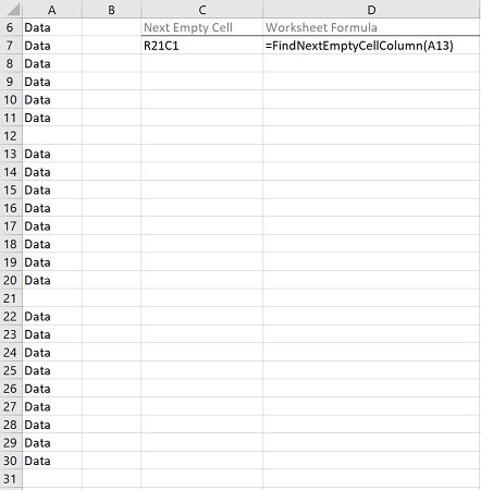
Example: Find next empty cell in column with VBA macros

#20. Excel VBA Find Value in Array

VBA Code to Find Value in Array

To find a numeric value in a one-dimensional array, use the following structure/template in the applicable procedure:

Dim PositionOfValueInArray As Variant
Dim LoopCounter As Long
PositionOfValueInArray = OutputIfValueNotInArray
For LoopCounter = LBound(SearchedArray) To UBound(SearchedArray)
    If SearchedArray(LoopCounter) = SearchedValue Then
        PositionOfValueInArray = LoopCounter
        Exit For
    End If
Next LoopCounter

The following Sections describe the main elements in this structure.

Lines #1 and #2: Dim PositionOfValueInArray As Variant | Dim LoopCounter As Long

The Dim statement:

Declares variables.
Allocates storage space.

PositionOfValueInArray | LoopCounter

The names of the variables declared with the Dim statement.

PositionOfValueInArray holds/represents:
- The position of the searched numeric value in the array, if the searched numeric value is found in the array.
- The default/fallback output/data, if the searched numeric value isn’t found in the array.
LoopCounter represents the loop counter used in the For… Next loop in lines #4 to #9.

As Variant | As Long

The data type of the variables declared with the Dim statement.

PositionOfValueInArray is of the Variant data type. The Variant data type can (generally) contain any type of data, except for fixed-length Strings.
LoopCounter is of the Long data type. The Long data type can contain integers between -2,147,483,648 and 2,147,483,647.

Line #3: PositionOfValueInArray = OutputIfValueNotInArray

PositionOfValueInArray

Variable holding/representing:

The position of the searched numeric value in the array, if the searched numeric value is found in the array.
The default/fallback output/data, if the searched numeric value isn’t found in the array.

=

The assignment operator assigns the result returned by an expression (OutputIfValueNotInArray) to a variable (PositionOfValueInArray).

OutputIfValueNotInArray

Expression specifying the default/fallback output/data to be assigned to the PositionOfValueInArray variable if the searched numeric value isn’t found in the array.

Lines #4 and #9: For LoopCounter = LBound(SearchedArray) To UBound(SearchedArray) | Next LoopCounter

For… = … To … | Next…

The For… Next statement repeats a series of statements a specific number of times.

LoopCounter

Variable holding/representing the loop counter.

LBound(…) | UBound(…)

The LBound/UBound functions return the lower/upper bound of an array’s dimension. The LBound/UBound functions accept two arguments:

ArrayName: The name of the array whose lower/upper bound you want to obtain.
Dimension:
- An optional argument.
- The dimension (of the applicable array) whose lower/upper bound you want to obtain.

If you omit specifying the Dimension argument, the LBound/UBound functions return the lower/upper bound of the array’s first dimension.

The initial/final values of LoopCounter are set to the following:

Initial value (Start) of LoopCounter: The output returned by the LBound function (LBound(SearchedArray)).
Final value (End) of LoopCounter: The output returned by the UBound function (UBound(SearchedArray)).

SearchedArray

The array you search in.

SearchedArray is passed as the ArrayName argument of the LBound/UBound functions.

Lines #5 and #8: If SearchedArray(LoopCounter) = SearchedValue Then | End If

If… Then… End If

The If… Then… Else statement:

Conditionally executes a set of statements (lines #6 and #7);
Depending on an expression’s value (SearchedArray(LoopCounter) = SearchedValue).

SearchedArray(LoopCounter) = SearchedValue

The condition of an If… Then… Else statement is an expression evaluating to True or False.

If the expression returns True, a set of statements (lines #6 and #7) is executed.
If the expression returns False:
- No statements are executed.
- Execution continues with the statement following End If (line #8).

In this expression:

SearchedArray: The array you search in.
LoopCounter: Variable holding/representing the loop counter.
SearchedArray(LoopCounter): Array element whose index number is LoopCounter.
=: The equal to comparison operator returns True or False as follows:
- True if both expressions (SearchedArray(LoopCounter) and SearchedValue) are equal.
- False if the expressions (SearchedArray(LoopCounter) and SearchedValue) are not equal.
SearchedValue: Numeric value you search for in the array (SearchedArray).

Line #6: PositionOfValueInArray = LoopCounter

PositionOfValueInArray

Variable holding/representing:

The position of the searched numeric value in the array, if the searched numeric value is found in the array.
The default/fallback output/data, if the searched numeric value isn’t found in the array.

=

The assignment operator assigns the result returned by an expression (LoopCounter) to a variable (PositionOfValueInArray).

LoopCounter

Variable holding/representing the loop counter.

Line #7: Exit For

The Exit For statement:

Exits a For… Next loop.
Transfers control to the statement following the Next statement (line #8).

Macro Example to Find Value in Array

The following macro (User-Defined Function) example does the following:

Accepts two arguments:
1. MyArray: The array you search in.
2. MyValue: The numeric value you search for.
Loops through each element in MyArray and tests whether the applicable element is equal to MyValue.
Returns the following:
1. If MyValue is not found in MyArray, the string “Value not found in array”.
2. If MyValue is found in MyArray, the position/index number of MyValue in MyArray.

Function FindValueInArray(MyArray As Variant, MyValue As Variant) As Variant
    'Source: https://powerspreadsheets.com/
    'For further information: https://powerspreadsheets.com/excel-vba-find/
    
    'This UDF:
        '(1) Accepts 2 arguments: MyArray and MyValue
        '(2) Loops through each element in the array (MyArray) and tests whether the applicable element is equal to the searched value (MyValue)
        '(3) Returns the following (as applicable):
            'If MyValue is not found in MyArray: The string "Value not found in array"
            'If MyValue is found in MyArray: The position (index number) of MyValue in MyArray
    
    'Declare variable to represent loop counter
    Dim iCounter As Long

    'Specify default/fallback value/string to be returned ("Value not found in array") if MyValue is not found in MyArray
    FindValueInArray = "Value not found in array"

    'Loop through each element in the array (MyArray)
    For iCounter = LBound(MyArray) To UBound(MyArray)
    
        'Test if the current array element is equal to MyValue
        If MyArray(iCounter) = MyValue Then
            
            'If the current array element is equal to MyValue:
                '(1) Return the position (index number) of the current array element
                '(2) Exit the For... Next loop
            FindValueInArray = iCounter
            Exit For
            
        End If
        
    Next iCounter

End Function

Effects of Executing Macro Example to Find Value in Array

To illustrate the effects of using the macro (User-Defined Function) example, I use the following macro. The following macro does the following:

Declare an array (MySearchedArray).
Fill the array with values (0, 10, 20, …, 90).
Call the FindValueInArray macro (User-Defined Function) example to find the number “50” in the array.
Display a message box with the value/string returned by the FindValueInArray macro (User-Defined Function) example.

Sub FindValueInArrayCaller()
    'Source: https://powerspreadsheets.com/
    'For further information: https://powerspreadsheets.com/excel-vba-find/
    
    'This procedure:
        '(1) Declares an array and fills it with values (0, 10, 20, ..., 90)
        '(2) Calls the FindValueInArray UDF to find the number "50" in the array
        '(3) Displays a message box with the value/string returned by the FindValueInArray UDF
    
    'Declare a zero-based array with 10 elements of the Long data type
    Dim MySearchedArray(0 To 9) As Long
    
    'Assign values to array elements
    MySearchedArray(0) = 0
    MySearchedArray(1) = 10
    MySearchedArray(2) = 20
    MySearchedArray(3) = 30
    MySearchedArray(4) = 40
    MySearchedArray(5) = 50
    MySearchedArray(6) = 60
    MySearchedArray(7) = 70
    MySearchedArray(8) = 80
    MySearchedArray(9) = 90
    
    'Do the following:
        '(1) Call the FindValueInArray UDF and search for the number "50" in MySearchedArray
        '(2) Display a message box with the value/string returned by the FindValueInArray UDF
    MsgBox FindValueInArray(MySearchedArray, 50)
    

End Sub

The following GIF illustrates the effects of using the macro above to call the macro (User-Defined Function) example.

As expected, this results in Excel displaying a message box with the number 5. This is the position of the searched numeric value (50) in the array.

Example: Find value in array with VBA macros

Learn More About Excel VBA Find

Workbook Example Used in this Excel VBA Find Tutorial

This VBA Find Tutorial is accompanied by an Excel workbook containing the data and macros I use in the examples above. You can get free access to this example workbook by clicking the button below.

The Power Spreadsheets Library

The Books at The Power Spreadsheets Library are comprehensive and actionable guides for professionals who want to:

Automate Excel;
Save time for the things that really matter; and
Open new career opportunities.

Learn more about The Power Spreadsheets Library here.

Источник