
Excel for Microsoft 365 Excel for Microsoft 365 for Mac Excel for the web Excel 2021 Excel 2021 for Mac Excel 2019 Excel 2019 for Mac Excel 2016 Excel 2016 for Mac Excel 2013 Excel 2010 Excel 2007 Excel for Mac 2011 Excel Starter 2010 More…Less
This article describes the formula syntax and usage of the FIND and FINDB functions in Microsoft Excel.
Description
FIND and FINDB locate one text string within a second text string, and return the number of the starting position of the first text string from the first character of the second text string.
Important:
-
These functions may not be available in all languages.
-
FIND is intended for use with languages that use the single-byte character set (SBCS), whereas FINDB is intended for use with languages that use the double-byte character set (DBCS). The default language setting on your computer affects the return value in the following way:
-
FIND always counts each character, whether single-byte or double-byte, as 1, no matter what the default language setting is.
-
FINDB counts each double-byte character as 2 when you have enabled the editing of a language that supports DBCS and then set it as the default language. Otherwise, FINDB counts each character as 1.
The languages that support DBCS include Japanese, Chinese (Simplified), Chinese (Traditional), and Korean.
Syntax
FIND(find_text, within_text, [start_num])
FINDB(find_text, within_text, [start_num])
The FIND and FINDB function syntax has the following arguments:
-
Find_text Required. The text you want to find.
-
Within_text Required. The text containing the text you want to find.
-
Start_num Optional. Specifies the character at which to start the search. The first character in within_text is character number 1. If you omit start_num, it is assumed to be 1.
Remarks
-
FIND and FINDB are case sensitive and don’t allow wildcard characters. If you don’t want to do a case sensitive search or use wildcard characters, you can use SEARCH and SEARCHB.
-
If find_text is «» (empty text), FIND matches the first character in the search string (that is, the character numbered start_num or 1).
-
Find_text cannot contain any wildcard characters.
-
If find_text does not appear in within_text, FIND and FINDB return the #VALUE! error value.
-
If start_num is not greater than zero, FIND and FINDB return the #VALUE! error value.
-
If start_num is greater than the length of within_text, FIND and FINDB return the #VALUE! error value.
-
Use start_num to skip a specified number of characters. Using FIND as an example, suppose you are working with the text string «AYF0093.YoungMensApparel». To find the number of the first «Y» in the descriptive part of the text string, set start_num equal to 8 so that the serial-number portion of the text is not searched. FIND begins with character 8, finds find_text at the next character, and returns the number 9. FIND always returns the number of characters from the start of within_text, counting the characters you skip if start_num is greater than 1.
Examples
Copy the example data in the following table, and paste it in cell A1 of a new Excel worksheet. For formulas to show results, select them, press F2, and then press Enter. If you need to, you can adjust the column widths to see all the data.
|
Data |
||
|
Miriam McGovern |
||
|
Formula |
Description |
Result |
|
=FIND(«M»,A2) |
Position of the first «M» in cell A2 |
1 |
|
=FIND(«m»,A2) |
Position of the first «M» in cell A2 |
6 |
|
=FIND(«M»,A2,3) |
Position of the first «M» in cell A2, starting with the third character |
8 |
Example 2
|
Data |
||
|
Ceramic Insulators #124-TD45-87 |
||
|
Copper Coils #12-671-6772 |
||
|
Variable Resistors #116010 |
||
|
Formula |
Description (Result) |
Result |
|
=MID(A2,1,FIND(» #»,A2,1)-1) |
Extracts text from position 1 to the position of «#» in cell A2 (Ceramic Insulators) |
Ceramic Insulators |
|
=MID(A3,1,FIND(» #»,A3,1)-1) |
Extracts text from position 1 to the position of «#» in cell A3 (Copper Coils) |
Copper Coils |
|
=MID(A4,1,FIND(» #»,A4,1)-1) |
Extracts text from position 1 to the position of «#» in cell A4 (Variable Resistors) |
Variable Resistors |
Need more help?
Want more options?
Explore subscription benefits, browse training courses, learn how to secure your device, and more.
Communities help you ask and answer questions, give feedback, and hear from experts with rich knowledge.
Функция НАЙТИ (FIND) в Excel используется для поиска текстового значения внутри строчки с текстом и указать порядковый номер буквы с которого начинается искомое слово в найденной строке.
Содержание
- Что возвращает функция
- Синтаксис
- Аргументы функции
- Дополнительная информация
- Примеры использования функции НАЙТИ в Excel
- Пример 1. Ищем слово в текстовой строке (с начала строки)
- Пример 2. Ищем слово в текстовой строке (с заданным порядковым номером старта поиска)
- Пример 3. Поиск текстового значения внутри текстовой строки с дублированным искомым значением
Что возвращает функция
Возвращает числовое значение, обозначающее стартовую позицию текстовой строчки внутри другой текстовой строчки.
Синтаксис
=FIND(find_text, within_text, [start_num]) — английская версия
=НАЙТИ(искомый_текст;просматриваемый_текст;[нач_позиция]) — русская версия
Аргументы функции
- find_text (искомый_текст) — текст или строка которую вы хотите найти в рамках другой строки;
- within_text (просматриваемый_текст) — текст, внутри которого вы хотите найти аргумент find_text (искомый_текст);
- [start_num] ([нач_позиция]) — число, отображающее позицию, с которой вы хотите начать поиск. Если аргумент не указать, то поиск начнется сначала.
Дополнительная информация
- Если стартовое число не указано, то функция начинает поиск искомого текста с начала строки;
- Функция НАЙТИ чувствительна к регистру. Если вы хотите сделать поиск без учета регистра, используйте функцию SEARCH в Excel;
- Функция не учитывает подстановочные знаки при поиске. Если вы хотите использовать подстановочные знаки для поиска, используйте функцию SEARCH в Excel;
- Функция каждый раз возвращает ошибку, когда не находит искомый текст в заданной строке.
Примеры использования функции НАЙТИ в Excel
Пример 1. Ищем слово в текстовой строке (с начала строки)

На примере выше мы ищем слово «Доброе» в словосочетании «Доброе Утро». По результатам поиска, функция выдает число «1», которое обозначает, что слово «Доброе» начинается с первой по очереди буквы в, заданной в качестве области поиска, текстовой строке.
Больше лайфхаков в нашем Telegram Подписаться
Обратите внимание, что так как функция НАЙТИ в Excel чувствительна к регистру, вы не сможете найти слово «доброе» в словосочетании «Доброе утро», так как оно написано с маленькой буквы. Для того, чтобы осуществить поиска без учета регистра следует пользоваться функцией SEARCH.
Пример 2. Ищем слово в текстовой строке (с заданным порядковым номером старта поиска)
Третий аргумент функции НАЙТИ указывает позицию, с которой функция начинает поиск искомого значения. На примере выше функция возвращает число «1» когда мы начинаем поиск слова «Доброе» в словосочетании «Доброе утро» с начала текстовой строки. Но если мы зададим аргумент функции start_num (нач_позиция) со значением «2», то функция выдаст ошибку, так как начиная поиск со второй буквы текстовой строки, она не может ничего найти.
Если вы не укажете номер позиции, с которой функции следует начинать поиск искомого аргумента, то Excel по умолчанию начнет поиск с самого начала текстовой строки.
Пример 3. Поиск текстового значения внутри текстовой строки с дублированным искомым значением
На примере выше мы ищем слово «Доброе» в словосочетании «Доброе Доброе утро». Когда мы начинаем поиск слова «Доброе» с начала текстовой строки, то функция выдает число «1», так как первое слово «Доброе» начинается с первой буквы в словосочетании «Доброе Доброе утро».
Но, если мы укажем в качестве аргумента start_num (нач_позиция) число «2» и попросим функцию начать поиск со второй буквы в заданной текстовой строке, то функция выдаст число «6», так как Excel находит искомое слово «Доброе» начиная со второй буквы словосочетания «Доброе Доброе утро» только на 6 позиции.
A few days back I had a huge spreadsheet in which I had to find out the cells containing formulas. Initially, I was totally clueless about how this task can be done.
But later after doing some Google searches, I got a few ideas on how I can effortlessly identify the formula cells in excel.
And today to share my experiences with you guys, In this post I will throw some light on a few methods that can help you to find out formula cells in your spreadsheets.
So here we go:
Method 1: Using ‘Go To Special’ Option:
In Excel ‘Go To Special’ is a very handy option when it comes to finding the cells with formulas. ‘Go to Special’ option has a radio button “Formulas” and selecting this radio button enables it to select all the cells containing formulas.
Later you can change the formatting or background color of the selected cells to make them stand out from the rest. Below is the step by step instructions for accomplishing this:
1. With your excel sheet opened navigate to the ‘Home’ tab > ‘Find & Select’ > ‘Go To Special’. Alternatively, you can also press ‘F5’ and then ‘Alt + S’ to open the ‘Go to Special’ dialog.

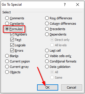
2. Next, in the ‘Go to Special’ window select the ‘Formulas’ radio button. After checking this radio button you will notice that few checkboxes (like Numbers, Errors, Logical, and Text) are enabled, these checkboxes signify the return type of the formulas.
So, if you select the ‘Formulas’ radio button and only check the ‘Numbers’ checkbox then it will just search the Formulas whose return type is a number. Here in our example, we will keep all of these return types checked.
3. After this click the ‘Ok’ button and all the cells that contain formulas get selected.
4. Next, without clicking anywhere on your spreadsheet change the background color of all the selected cells.
5. Now your formula cells can be easily identified.
Method 2: Using a built-in Excel formula
If you have worked with excel formulas then probably you may be knowing that excel has a formula that can find whether a cell contains a formula or not. The formula that I am talking about is:
=ISFORMULA(reference)
Here ‘reference’ signifies the cell position which you wish to check for the presence of a formula.
For example: If you wish to check the cell ‘A2’ for the existence of a formula then you can use this function as
=ISFORMULA(A2)
This function results in a Boolean output i.e. True or False. True signifies that the cell contains formulas while False tells that cell doesn’t contain any formulas.
Method 3: Using a Macro for identifying the cells that contain formulas:
I have created a VBA Macro that can find and color any cells that contain the formula in the total used range of the Active sheet. To use this macro simply follow the below procedure:
1. Open your spreadsheet and hit the ‘Alt + F11’ keys to open the VBA editor.

2. Next, navigate to ‘Insert‘ > ‘Module‘ and then paste the below macro in the editor.
Sub FindFormulaCells()
For Each cl In ActiveSheet.UsedRange
If cl.HasFormula() = True Then
cl.Interior.ColorIndex = 24
End If
Next cl
End Sub
3. For running this formula press the “F5” key.
4. This Macro will change the background colour of all the formula containing cells and thus makes it easier to identify them easily.
Recommended Reading: How to add a Checkbox in excel
Purpose
Get location substring in a string
Return value
A number representing the location of substring
Usage notes
The FIND function returns the position (as a number) of one text string inside another. If there is more than one occurrence of the search string, FIND returns the position of the first occurrence. When the text is not found, FIND returns a #VALUE error. Also note, when find_text is empty, FIND returns 1. FIND does not support wildcards, and is always case-sensitive. Use the SEARCH function to find the position of text without case-sensitivity and with wildcard support.
Basic Example
The FIND function is designed to look inside a text string for a specific substring. When FIND locates the substring, it returns a position of the substring in the text as a number. If the substring is not found, FIND returns a #VALUE error. For example:
=FIND("p","apple") // returns 2
=FIND("z","apple") // returns #VALUE!
Note that text values entered directly into FIND must be enclosed in double-quotes («»).
Case-sensitive
The FIND function always case-sensitive:
=FIND("a","Apple") // returns #VALUE!
=FIND("A","Apple") // returns 1
TRUE or FALSE result
To force a TRUE or FALSE result, nest the FIND function inside the ISNUMBER function. ISNUMBER returns TRUE for numeric values and FALSE for anything else. If FIND locates the substring, it returns the position as a number, and ISNUMBER returns TRUE:
=ISNUMBER(FIND("p","apple")) // returns TRUE
=ISNUMBER(FIND("z","apple")) // returns FALSE
If FIND doesn’t locate the substring, it returns an error, and ISNUMBER returns FALSE.
Start number
The FIND function has an optional argument called start_num, that controls where FIND should begin looking for a substring. To find the first match of «the» in any combination of upper or lowercase, you can omit start_num, which defaults to 1:
=FIND("x","20 x 30 x 50") // returns 4To start searching at character 5, enter 4 for start_num:
=FIND("x","20 x 30 x 50",5) // returns 9
Wildcards
The FIND function does not support wildcards. See the SEARCH function.
If cell contains
To return a custom result with the SEARCH function, use the IF function like this:
=IF(ISNUMBER(FIND(substring,A1)), "Yes", "No")
Instead of returning TRUE or FALSE, the formula above will return «Yes» if substring is found and «No» if not.
Notes
- The FIND function returns the location of the first find_text in within_text.
- The location is returned as the number of characters from the start.
- Start_num is optional and defaults to 1.
- FIND returns 1 when find_text is empty.
- FIND returns #VALUE if find_text is not found.
- FIND is case-sensitive but does not support wildcards.
- Use the SEARCH function to find a substring with wildcards.
The two formulas FIND and SEARCH in Excel are very similar. They search through a cell or some text for a keyword or character. Once found, they return the number of characters, at which the keyword starts. Let’s learn how to use them and explore the differences of the two formulas.
How to use the FIND formula
The formula returns the number of the character, at which your search term starts. If your text can’t be found, it’ll return a “#VALUE” error.
Structure of the FIND formula
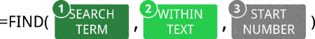
The structure of the FIND formula is quite simple (the numbers are corresponding to the image on the right-hand side):
- SEARCH TERM: The first part of the formula is the text you look for.
- WITHIN TEXT: The cell or text you want to search your “SEARCH TERM” in.
- START NUMBER: This argument is optional. If you don’t want to start searching at the beginning of the text, fill in the number larger than 1, otherwise just type 1 or leave it blank.
If you just want to know, if your text can be found within another cell, you might want to go with the following formula. B2 contains the text or character you search for and B3 is the cell you search in:
=IFERROR(IF(FIND(B2,B3)>0,”Value found”,””),”Value not found”)
Please note the following comments:
- FIND is case-sensitive. That means, it matters if you use small or capital letters.
- You can also search for numbers within another number. For example: =FIND(1,321)This formula returns 3 because the number 1 is the third character of 321.
- You can’t use wildcard criteria (“*” or “?”) with the FIND formula.
- Please refer to this article if you want to know more about the IF formula and to this article for more information about the IFERROR formula.
Examples for the FIND formula
Let’s try some examples.
Example 1: Find the first occurrence
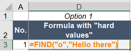
The “default” usage of the FIND formula is to return the number of characters, at which a text first occurs within another text. Let’s say you have the text “Hello there” and want to know, at which position you have an “o”. In such case, you write the following formula (example number 1 in the Excel workbook you can download at the end of this article).
=FIND(“o”,”Hello there”)
The return value is 5.
Example 2: Find the first occurrence after the third character
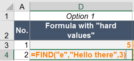
Another example: You want to know the position of “e” after the third character (example number 2 in the example workbook).
=FIND(“e”,”Hello there”,3)
The return value is 9.
Example 3: Find the second occurrence
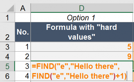
Now you want to know the position of the second occurrence of “e” in “Hello there”.
=FIND(“e”;”Hello there”;FIND(“e”;”Hello there”)+1)
This formula works as follows. The second FIND formula returns the position of the first occurrence of “e” in “Hello there” which is 2. This is used as the START NUMBER (+ 1 because you want to start counting after the first “e”) for the first FIND formula.
Example 4: Find the last occurrence
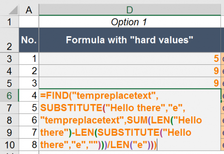
Finding the last occurrence of a string within a text is a little bit more complicated. You use SUBSTITUTE and LEN. The complete formula is like this:
=FIND(“tempreplacetext”;SUBSTITUTE(“Hello there”;”e”;”tempreplacetext”;SUM(LEN(“Hello there”)-LEN(SUBSTITUTE(“Hello there”;”e”;””)))/LEN(“e”)))
In order to understand the formula better, let’s start in the middle with the part SUM(LEN(“Hello there”)-LEN(SUBSTITUTE(“Hello there”;”e”;””)))/LEN(“e”)))
This part of the formula determines the number of “e” in “Hello there”. It replaces “e” in “Hello there” and the difference in the two versions (with and without e – “Hello there” and “Hllo thr”) is the number of “e”s.
The whole part SUBSTITUTE(“Hello there”;”e”;”tempreplacetext”;SUM(LEN(“Hello there”)-LEN(SUBSTITUTE(“Hello there”;”e”;””)))/LEN(“e”))) replaces the last “e” by “tempreplacetext”. Now you just put this into the FIND formula and get the position of “tempreplacetext”.
If you want to use this formula, replace all “e”s by your cell reference for the SEARCH TEXT and all “Hello there” by the cell reference to your WITHIN TEXT.
Replace text enclosed by brackets
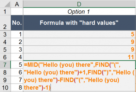
A last example for the FIND formula: You want to know what is written between two brackets. In such case, you can also use the FIND formulas in combination with the MID formula.
=MID(“Hello (you) there”,FIND(“(“,”Hello (you) there”)+1,FIND(“)”,”Hello (you) there”)-FIND(“(“,”Hello (you) there”)-1)
The MID formula returns some part of text from a (longer) text. It has three arguments:
- The initial, complete text.
- The starting character for the text you want to get.
- The length (in number of characters) of text you want to extract.
In our example above, the first FIND formula provides the character you want to start at. In our case that’s the first opening bracket (+1 because you want to start one character later). The second and third FIND formulas determine the length by
How to use the SEARCH formula
Like the FIND formula in Excel, SEARCH also returns the position of a text within another text.
Structure of the SEARCH formula

The SEARCH formula is very similar to the FIND formula. It has exactly the same arguments and works the same way.
Because of the, the structure is as follows:
- The SEARCH TERM is the text or character you search for.
- WITHIN TEXT contains the text you search in.
- The START NUMBER is optional and defines the number of character, after which Excel should start searching.
Yes, you are right – these arguments are exactly the same like in the FIND formula. But there is a major difference: SEARCH does not regard lower and upper case: It is not case sensitive. FIND on the other hand is case-sensitive and regards upper and lower cases.
Do you want to boost your productivity in Excel?
Get the Professor Excel ribbon!

Add more than 120 great features to Excel!
Examples for the SEARCH formula
The examples work exactly the same way like for the FIND formula. You only have to replace “FIND” by “SEARCH”. Because of that, we just show the summary below. If you want to know more, either scroll up to the “FIND”-examples or download the example workbook below.
| Example no. | Description | Formula |
| 6 | Return the position of “o” in “Hello there”. | =SEARCH(“o”,”Hello there”) |
| 7 | Return the position of “e” in “Hello there” after the third character. | =SEARCH(“e”,”Hello there”,3) |
| 8 | Return the position of the second occurrence of “e” in “Hello there”. | =SEARCH(“e”,”Hello there”,SEARCH(“e”,”Hello there”)+1) |
| 9 | Return the position of the last occurrence of “e” in “Hello there”. | =SEARCH(“tempreplacetext”,SUBSTITUTE(“Hello there”,”e”,”tempreplacetext”,SUM(LEN(“Hello there”)-LEN(SUBSTITUTE(“Hello there”,”e”,””)))/LEN(“e”))) |
| 10 | Return the text within brackets of “Hello (you) there”. | =MID(“Hello (you) there”,SEARCH(“(“,”Hello (you) there”)+1,SEARCH(“)”,”Hello (you) there”)-SEARCH(“(“,”Hello (you) there”)-1) |
Troubleshooting
The error message “#VALUE!” comes up most often for the FIND and SEARCH formulas. If you receive a “#VALUE!” error, please check the following possibilities.
- Make sure your SEARCH TERM can be found. If it can’t be found, you’ll receive the #VALUE! error.
- The last argument, the START NUMBER, is larger than the number of characters of in your WITHIN TEXT argument.
- You haven’t provided the last argument although you wrote the comma. For instance =SEARCH(“b”,”abc”,).
- Please check, if your SEARCH TERM and WITHIN TEXT have the same format. You can’t search for a letter or text in a number cell.
Difference between FIND and SEARCH
The first and major difference between FIND and SEARCH:
FIND is case-sensitive. SEARCH is not case-sensitive.
That means, FIND regards capital and small letter whereas SEARCH doesn’t.
How to remember which is which? I use the mnemonic:
- FIND finds exactly what you look for.
- Searching for something also searches for roughly what you look for.
I admit, it’s not the best mnemonic. Please let me know, if you have a better one!
There is also a second difference between FIND and SEARCH: You can use SEARCH with wildcard criteria within the SEARCH TERM.
- “?” stands for a single character. Example: =SEARCH(“?b”,”abc”)
- “*” matches any sequence of characters. =SEARCH(“*b”,”abc”)
- If you want to search exactly for ? or *, write a tilde in front of them. Example: =SEARCH(“~*”,”ab*c”)
Differences between FIND and FINDB as well as SEARCH and SEARCHB
Maybe you have noticed that there is also a slightly different version of the two formulas in Excel. If you add a “B” to the formulas, you can still use them the same way. So what is the difference?
FINDB and SEARCHB provide support for more complex languages. The definition by Microsoft is:
SEARCHB counts 2 bytes per character only when a DBCS language is set as the default language. Otherwise SEARCHB behaves the same as SEARCH, counting 1 byte per character.
According to Wikipedia DBCS stands mainly for the Asian languages Chinese, Japanese and Korean.
Please feel free to download all the examples shown above in this Excel file.
Click here and the download starts immediately.
The FIND function of Excel searches and returns the position of a character within a text string. This position is returned as a numeric value, which represents the first instance of such character. The FIND function can also be informed the exact position from where the search should begin.
For example, the formula =FIND(“w”,“sunflower”) returns 7. This implies that the character “w” is at the seventh position of the text string “sunflower.”
The FIND function searches within the text string beginning from left to right. The purpose of using the FIND function is to ascertain whether a particular substring occurs in a specific cell or not. The FIND can also be used with other Excel functionsExcel functions help the users to save time and maintain extensive worksheets. There are 100+ excel functions categorized as financial, logical, text, date and time, Lookup & Reference, Math, Statistical and Information functions.read more to extract certain characters of a text string.
The FIND function is categorized as a Text function of Excel.
Table of contents
- What is FIND Function in Excel?
- Syntax of the FIND Function of Excel
- How to use the FIND Function in Excel?
- Example #1–Find a Single Character Within a Text String
- Example #2–Count the Number of Times a Single Character Occurs in a Range
- Example #3–Count the Text Strings Ending With Certain Characters
- Example #4–Extract Certain Characters From Each Cell of a Range
- Relevance and Uses of the FIND Function of Excel
- The Key Points Related to the FIND Function of Excel
- Frequently Asked Questions
- FIND Function in Excel Video
- Recommended Articles
Syntax of the FIND Function of Excel
The syntax of the FIND function of Excel is shown in the following image:

The FIND function of Excel accepts the following arguments:
- Find_text: This is the character (or substring) whose position is to be searched. It can be supplied as a reference to a cell containing the substring or as a direct substring enclosed within double quotation marks.
- Within_text: This is the text string within which the character (or substring) needs to be searched. It can be supplied either directly to the FIND function or as a reference to a cell containing the text string. Enclose the text string within double quotation marks when supplied directly to the function.
- Start_num: This is the character from which the search shall begin. It is supplied as a numeric value to the FIND function. For instance, if this argument is 3, the search begins from the third character of the “within_text” argument.
The arguments “find_text” and “within_text” are required, while “start_num” is optional. If the “start_num” argument is omitted, the search begins from the first character of the “within_text” argument.
How to use the FIND Function in Excel?
Let us consider some examples to understand the working of the FIND function in Excel.
You can download this FIND Function Excel Template here – FIND Function Excel Template
Example #1–Find a Single Character Within a Text String
The following image shows a text string and substring in cells A3 and B3 respectively. Within the text string (leopard), we want to find the substring (a) by using the FIND function of Excel. Supply the “find_text” and “within_text” arguments as:
- Cell references
- Direct strings
Consider the “start_num” argument to be 1 in both cases.

a. The steps to use the FIND function with cell referencesCell reference in excel is referring the other cells to a cell to use its values or properties. For instance, if we have data in cell A2 and want to use that in cell A1, use =A2 in cell A1, and this will copy the A2 value in A1.read more are listed as follows:
Step 1: Supply the cell references of the substring and the text string (in the stated sequence) to the FIND function. So, enter the following formula in cell C3.
“=FIND(B3,A3)”
Notice that the “start_num” argument is omitted since it is 1.

Step 2: Press the “Enter” key. The output appears, as shown in the following image. Hence, the character “a” is the fifth letter of the word “leopard.”

b. The steps to use the FIND function with direct strings are listed as follows:
Step 1: Supply the substring and the text string (in the stated sequence) to the FIND function directly. So, enter the following formula in cell C4.
“=FIND(“a”, “Leopard”)”
Since the “start_num” argument is 1, it has been omitted.

Step 2: Press the “Enter” key. The output in cell C4 is 5. This is shown in the following image. Hence, whether the first two arguments are entered as cell references or direct strings, the output of the FIND function is the same.

Example #2–Count the Number of Times a Single Character Occurs in a Range
The following image shows some random text strings in the range A3:A6. We want to find the number of times the character (or substring) “i” appears in this range. Use the FIND, ISNUMBER, and SUMPRODUCT functions of Excel.

The steps to find the character count by using the stated functions are listed as follows:
Step 1: Enter the following formula in cell B3.
“=SUMPRODUCT(- -(ISNUMBER(FIND(“i”,A3:A6))))”

Step 2: Press the “Enter” key. The output in cell B3 is 3. This is shown in the following image. Hence, the character “i” appears thrice in the range A3:A6.

Explanation: In the formula entered in step 1, the FIND function is processed first as it is the innermost function. Next, the ISNUMBERISNUMBER function in excel is an information function that checks if the referred cell value is numeric or non-numeric.read more and SUMPRODUCTThe SUMPRODUCT excel function multiplies the numbers of two or more arrays and sums up the resulting products.read more functions are processed. The entire formula works as follows:
- The FIND function looks for the character “i” in each cell of range A3:A6. This character is found in cells A3, A4, and A6. It is not found in cell A5. If the character “i” is found in a cell, the FIND function returns its position. However, if this character is not found in a cell, the FIND function returns the “#VALUE!” error. So, the FIND function returns an array of four values {3;5;#VALUE!;5 }.
- The array returned by the FIND function becomes an argument of the ISNUMBER function. If the output of the FIND function is numeric, the ISNUMBER returns “true.” However, if the output of the FIND function is an error, the ISNUMBER function returns “false.” So, the ISNUMBER returns an array of Boolean values {TRUE;TRUE;FALSE;TRUE}.
- The unary operator or the double negative symbol (- -) converts every “true” and “false” output of the ISNUMBER function into 1 and 0 respectively. So, the unary operator returns a vertical array of four numbers {1;1;0;1}.
- The array ({1;1;0;1}) returned by the unary operator becomes an argument of the SUMPRODUCT function. Since it is a single array of numbers, the SUMPRODUCT sums it. So, the sum returned by the SUMPRODUCT function is 3.
Hence, the final output of the given formula (entered in step 1) is 3.
Notice that three cells of the range A3:A6 contained a single instance of the character “i.” However, had there been multiple occurrences of this character in cells A3, A4 or A6, the FIND function would have returned its first instance. Therefore, the final output would still have been 3.
Note 1: The ISNUMBER function checks whether a value (or a cell containing a value) is numeric or not. The SUMPRODUCT function multiplies the numbers of two or more arrays and sums up the resulting products. In case of a single array, the SUMPRODUCT function adds the numbers and returns their sum.
For the syntax of the ISNUMBER and SUMPRODUCT functions, click the hyperlinks given in the preceding explanation.
Note 2: Rather than the FIND function, one could have used the COUNTIFThe COUNTIF function in Excel counts the number of cells within a range based on pre-defined criteria. It is used to count cells that include dates, numbers, or text. For example, COUNTIF(A1:A10,”Trump”) will count the number of cells within the range A1:A10 that contain the text “Trump”
read more function. The formula for counting the character “i” in the range A3:A6 would be =COUNTIF(A3:A6,“*i*”). This formula would also have returned the output 3.
Like the FIND function, the COUNTIF would also have returned 3 in case of multiple occurrences of character “i” in cells A3, A4 or A6. However, the COUNTIF is not case-sensitive, unlike the FIND function.
Example #3–Count the Text Strings Ending With Certain Characters
The following image shows a list of names in column A. We want to find the number of names ending with “ansh” or “anka” in the range A3:A10. Use the FIND, ISNUMBER, and SUMPRODUCT functions of Excel.

The steps to count specific names by using the stated functions are listed as follows:
Step 1: Enter the following formula in cell B3.
“=SUMPRODUCT(- -((ISNUMBER(FIND(“ansh”,A3:A10))+ISNUMBER(FIND(“anka”,A3:A10)))>0))

Step 2: Press the “Enter” key. The output in cell B3 is 4. This is shown in the following image.
Hence, a total of 4 names end with “ansh” or “anka.” Two names end with the former substring (Priyansh and Divyansh) and two names end with the latter substring (Priyanka and Divyanka).

Explanation: The formula entered in step 1 is explained as follows:
- The FIND function processes each name of the range A3:A10. If “ansh” or “anka” are present in a cell, the FIND function returns the position of the first letter of these substrings. However, if these substrings are not present in a cell, the FIND function returns the “#VALUE!” error. So, the FIND function returns two arrays {#VALUE!;#VALUE!;5;5;#VALUE!;#VALUE!;#VALUE!; #VALUE!} and {5;5;#VALUE!;#VALUE!;#VALUE!;#VALUE!;#VALUE!;#VALUE!}.
- The ISNUMBER processes the outputs returned by the FIND function. If the output of the FIND function is numeric, the ISNUMBER returns “true,” otherwise returns “false.” So, the ISNUMBER function returns two arrays {FALSE;FALSE;TRUE;TRUE;FALSE;FALSE;FALSE;FALSE} and {TRUE;TRUE;FALSE;FALSE;FALSE;FALSE;FALSE;FALSE}.
- The two arrays returned by the ISNUMBER function are added due to the “plus” operator placed between them. The array returned after addition and the application of the “greater than zero” expression is {TRUE;TRUE;TRUE;TRUE;FALSE;FALSE;FALSE;FALSE}.
- The unary operator (- -) converts each “true” and “false” output of the preceding array to 1 and 0 respectively. So, the unary operator returns the final array of 8 values {1;1;1;1;0;0;0;0}.
- The SUMPRODUCT function sums the single array returned by the unary operator. Hence, this function returns the output 4.
Note 1: The “greater than zero” expression checks whether each output of the two arrays (returned by the ISNUMBER function) is greater than zero or not. This expression is useful in case one requires logical values (true and false) as the output.
This expression returns “true” if either of the two outputs (of the two arrays returned by the ISNUMBER function) is a number. It returns “false” if both outputs are errors.
Note 2: For knowing more about the ISNUMBER and SUMPRODUCT functions, refer to the hyperlinks (within the explanation) or “note 1” of the preceding example (example #2).
The following image shows some incomplete statements containing a hash symbol (#) in column C. From each statement, we want to extract this symbol, the word following it, and the trailing space in a separate column. Use the MID and FIND functions of Excel.

The steps to extract the given substrings using the stated functions are listed as follows:
Step 1: Enter the following formula in cell D3.
“=MID(C3,FIND(“#”,C3),FIND(” “,(MID(C3,FIND(“#”,C3),LEN(C3)))))”

Step 2: Press the “Enter” key. The output in cell D3 is “#Wedding .” It includes a space at the end. The output is shown in the following image.

Step 3: Drag the formula of cell D3 till cell D5 by using the fill handle. The output of the range D3 to D5 is shown in the following image.
Hence, the hash symbol, the following word, and the trailing space have been extracted from each statement of column C.

Explanation: In the given formula (entered in step 1), each function on the right is processed, followed by the subsequent function on the left. The LEN functionThe Len function returns the length of a given string. It calculates the number of characters in a given string as input. It is a text function in Excel as well as an inbuilt function that can be accessed by typing =LEN( and entering a string as input.read more, being the innermost (or rightmost), is processed first. The entire formula works as follows:
- The LEN function counts the total number of characters in cell C3. So, the formula “=LEN(C3)” returns 27. This count includes 23 letters, 3 spaces, and 1 hash symbol.
- Next, the FIND function searches the position of the hash symbol in cell C3. So, the formula “=FIND(“#”,C3)” returns 10. This implies that the hash symbol is at the tenth position of the statement given in cell C3.
- The outputs of the FIND and LEN functions become the arguments of the MID functionThe mid function in Excel is a text function that finds strings and returns them from any mid-part of the spreadsheet. read more. So, the MID function processes the formula “=MID(C3,10,27)” and returns “#Wedding in Jaipur.”
- The output of the MID function becomes the argument of the FIND function. The FIND function searches for a space character in the string “#Wedding in Jaipur.” So, the formula “=FIND(“ ”,“#Wedding in Jaipur”) returns 9. This implies that the first instance of the space character is at the ninth position of the given text string (#Wedding in Jaipur).
- The formula “=FIND(“#”,C3)” again returns 10.
- The outputs of the two FIND functions (in the preceding two pointers) become the arguments of the MID function. The formula “=MID(C3,10,9)” returns the string beginning from the tenth character and consisting of nine characters in total. So, this formula returns “#Wedding ” including a single space at the end of the word.
Likewise, the outputs in cells D4 and D5 have been returned by Excel.
Note 1: The LEN function counts all the characters in a cell. This includes letters, numbers, spaces, and special characters. The MID function helps extract a certain number of characters from the middle of the string. The position to begin extraction from can be specified to the MID function.
For the syntax of the LEN and MID functions, click the hyperlinks given in the preceding explanation.
Note 2: In the formula “=MID(C3,10,27),” the “start_num” argument is 10 and the “num_chars” argument is 27. If the sum of these two arguments exceeds the total length of the string, the MID function returns the characters beginning from the “start_num” till the end of the entire string.
Therefore, since 37 (“start_num” is 10 and “num_chars” is 27) exceeds 27 (length of the entire string), the MID function returns the character beginning from the tenth place (#) till the end of the string (Jaipur). So, the MID function returns “#Wedding in Jaipur.”
Relevance and Uses of the FIND Function of Excel
The FIND function of Excel is helpful in the following situations:
- It helps extract the relevant characters, thereby removing the unwanted substrings of a text string.
- It helps extract the words preceding or succeeding a specific character.
- It assists in searching the nth occurrence of a character.
- It can be combined with other functions of Excel to find the number of times a character appears in a range.
The important points related to the FIND function of Excel are listed as follows:
- The FIND function looks for the first occurrence of the “find_text” in the “within_text” argument.
- The “find_text” and “within_text” arguments can be supplied as cell references or direct text strings. To supply these arguments as direct text strings, they must be enclosed within double quotation marks.
- If the “find_text” argument contains more than one character, the FIND function returns the position of the first character in the “within_text” argument.
- If the “find_text” argument is an empty string (“”), the FIND function returns 1.
- The FIND function is case-sensitive and does not support the usage of wildcard characters.
- The FIND function returns the “#VALUE!” error in the following cases:
- The “find_text” is not found in the “within_text” argument
- The “start_num” argument is zero or negative
- The “start_num” argument contains more characters than the “within_text” argument
Frequently Asked Questions
1. Define the FIND function of Excel.
The FIND function of Excel returns the position of a character within a text string. The first instance of such character is returned. In case multiple characters are searched within a text string, the position of the first searched character is returned.
The FIND function of Excel returns a numeric value. The function can be told the position from where the search should begin.
Note: For the syntax of the FIND function of Excel, refer to the heading “syntax of the FIND function of Excel” of this article.
2. Is the FIND function of Excel case-sensitive? Explain with the help of an example.
Yes, the FIND function of Excel is case-sensitive. This implies that this function treats the lowercase and uppercase letters differently.
For example, the formula =FIND(“m”,“smile”) looks for the lowercase “m” in the text string “smile.” It returns 2, signifying that “m” is the second letter of the given text string.
However, the formula =FIND(“M”,“smile”) looks for the uppercase “M” in the text string “smile.” It returns the “#VALUE!” error since “M” could not be found in the given text string. Had the text string been supplied as “SMILE,” the FIND function would have again returned 2.
Note: For a case-insensitive function, use the SEARCH in place of the FIND function of Excel.
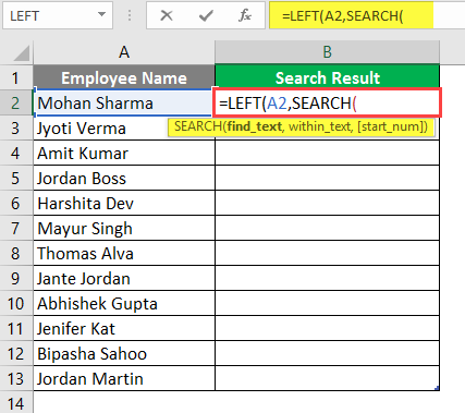
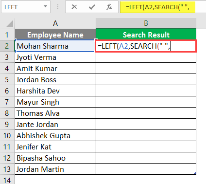
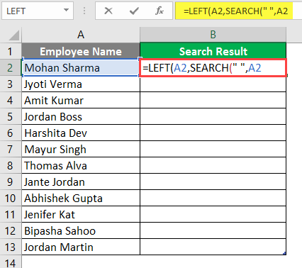
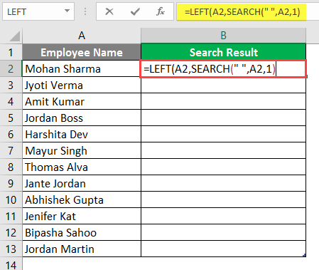
3. How can the FIND function be used with the LEFT function of Excel?
The LEFT function helps extract the specified number of characters from the leftmost side of a text string. The FIND and LEFT functions can be used together to extract a substring from the left side of a cell. The formula for the same is stated as follows:
“=LEFT(textstring,FIND(character,textstring)-1)”
The “textstring” is the cell reference containing the entire text string. The substring preceding the “character” is extracted. The “-1” ensures that the “character” is not included in the output.
Therefore, if the substring “rose” needs to be extracted from cell A1 containing “rose flower,” the formula used is “=LEFT(A1,FIND(” “,A1)-1).” The “-1” of the formula helps exclude the trailing space of the substring extracted. Had the strings “rose” and “flower” been separated by a hyphen, we would have used the hyphen (“-”) as the “character.”
Note: The given formula should be entered in Excel without the beginning and ending double quotation marks.
FIND Function in Excel Video
Recommended Articles
This has been a guide to the FIND function in Excel. Here we discuss how to use FIND Formula in excel along step by step examples. You may also look at these useful functions in Excel–
- Excel Find and SelectFind and Select in Excel is a feature available on the Home Tab of Excel that facilitates the user to quickly discover a specific text or value in the given data. The shortcut key to instantly use this feature is Ctrl+F.read more
- VBA FIND FunctionVBA Find gives the exact match of the argument. It takes three arguments, one is what to find, where to find and where to look at. If any parameter is missing, it takes existing value as that parameter.read more
- Row Function in ExcelThe row function in Excel is a worksheet function that displays the current row index number of the selected or target cell. The syntax to use this function is as follows: =ROW( Value ).read more
- VLOOKUP Excel FunctionThe VLOOKUP excel function searches for a particular value and returns a corresponding match based on a unique identifier. A unique identifier is uniquely associated with all the records of the database. For instance, employee ID, student roll number, customer contact number, seller email address, etc., are unique identifiers.
read more
This post will guide you how to use Excel FIND function with syntax and examples in Microsoft excel.
Table of Contents
- Description
- Syntax
- Excel Find Function Examples
- Frequently Asked Questions
- Related Functions
- More FIND Formula Examples in Excel
Description
The Excel FIND function returns the position of the first text string (sub string) within another text string.
It can be used when you want to get the position of a sub string inside another text string. so it will return a number that indicates the starting position of sub string that you are searching in another text string.
The FIND function is a build-in function in Microsoft Excel and it is categorized as a Text Function.
Note: The FIND Function is case-sensitive.
The FIND function is available in Excel 2016, Excel 2013, Excel 2010, Excel 2007, Excel 2003, Excel xp, Excel 2000, Excel 2011 for Mac.
Syntax
The syntax of the FIND function is as below:
= FIND(find_text, within_text,[start_num])
Where the FIND function arguments are:
- Find_text -This is a required argument. The text or substring that you want to find. (The string in the Find_text argument can not contain any wildcard characters)
- within_text -This is a required argument. The text string that is to be searched
- start_num-This is an optional argument. It will specify the position in within text string where the search will start. If you omit start_num value, the search will start from the first character of the within_text string, in other words, it is set to be 1 by default. So you can use the Excel Find function to look for the specified text starting from the specified position.
Note:
- The Find function will return the position of the first character of find_text in within_text argument.
- If there are several occurrences of the find_text within another text string, it only return the position of the first occurrence.
- If the find_text is an empty string, the position of the first character in the within_text is returned.
- If the find_text string is not found in within_text, it will return the Excel #VALUE! Error.
- If start_number value is not greater than 0, it will return the #VALUE! Error value.
- As the FIND function is case-sensitive. If you want to do a search that is case-insensitive , you can use the SEARCH Function.
- The FIND function does not support wildcard characters, so if you want to use wildcard characters to find string, you can use SEARCH function in excel.
Excel Find Function Examples
The below example will show you how to use Excel FIND Text function to find the position of a sub string within text string.
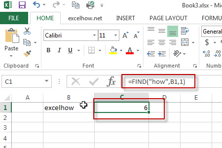
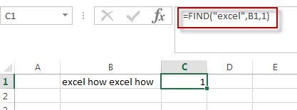
#1 To get the position of sub string “how” in cell B1, just using formula:
=FIND("how",B1,1).
When you look for the text “how” in the Cell B1, it will return 6, which is the position of the first character of find_text “how” within the Cell B1.
#2 To get the position of sub string “how”in cell b1, starting with the third character, using formula:
=FIND("how",B1,3)
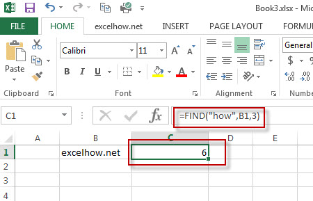
In the above example, it specified the start_num value as “3“, so you will get the position of the first character “h” of the searched string “how” within the value in Cell B1 when the starting position is 3. it returns 6.
The Example 1The search will start from the third character of the value in Cell B1.
#3 Finding “excel” string in Cell B1, using the following Find formula:
=FIND("excel",B1,1)
=FIND("excel",B1,3)
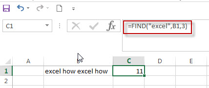
when you set the starting position as 1, it will return the position of the first “excel” string in the value of Cell B1.
When you set the starting position as 3, it will return the position of the second “excel” string in the value of Cell B1. The search will start from the third character of the value in Cell B1.
#4 Searching an empty string in Cell B1, using the following Find formula:
=FIND("",B1,1)
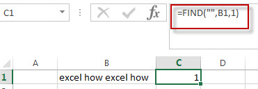
In the above example, when you look for an empty string in Cell B1 with the starting position as 1, and it will return the position of the first character of the within_ text (the value of Cell B1).
#5 Searching “word” text in Cell B1, using the following Find formula:
=FIND("word", B1,1)
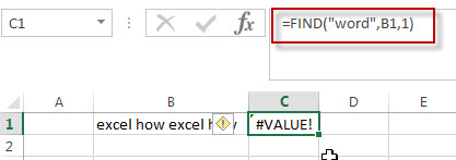
In the above example, when you look for the text “word” in Cell B1 and the string position is 1, it will return a #VALUE! error, As the searched string “word” is not found in Cell B1.
#6 Searching for a text as “excel” in Cell B1 and the starting position is a negative number.
=FIND("excel",B1,-1)
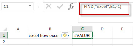
If the starting position is not greater than 0, it will return a #VALUE! Error.
#7 Searching for a string as “EXCEL” in Cell B1, using the following formula:
=FIND("EXCEL",B1,1)
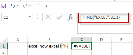
As the FIND function in excel is case-sensitive, when you look for the string “EXCEL” in Cell B1, the searched string “EXCEL” is not found, the function will return a #VALUE! error.
Frequently Asked Questions
Question 1: the FIND function returns a #VALUE error when it do not find the searched text within another string. I want to know if there is another excel function in combination with the find function to handle the error message to return the actual value, such as: -1 or throwing others exceptions via returning values, like: -1,0 or FALSE.
Answer: As mentioned above, the FIND function is case-sensitive, and it can be combined with the ISNUMBER function and IF function to create a new IF excel formula as follows:
=IF(ISNUMBER( FIND("excel",B1)), FIND("excel",B1), "not found")
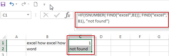
The FIND function will locate the position of the searched text “excel” within Cell B1, and the ISNUMBER function will check the result returned by the FIND function if it is a number, if TRUE, then return TRUE, otherwise , returns FALSE. then the IF will check the Boolean value returned by ISNUMBER function, If TRUE, then returns the numeric position returned by the second FIND function, If FALSE, returns “not found” string.
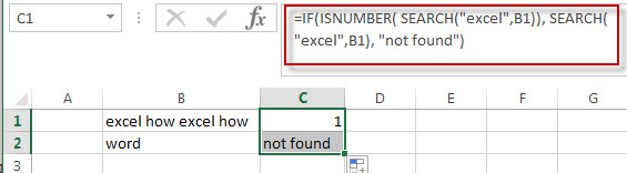
If you want a case-insensitive match and you can use the SEARCH function instead of the FIND function in the above formula:
=IF(ISNUMBER( SEARCH("excel",B1)), SEARCH("excel",B1), "not found")
Question 2: I want to extract a sub string from a string that separated by wildcard characters. I tried to use the below FIND formula to handle it. but it returned a #VALUE error message. Could you please help to check the below formula I used:
=RIGHT(B1,FIND("~**",B1))
Answer: you can use the following formula:
=TRIM(RIGHT(B1,Len(B1) - FIND("**",B1)-1))
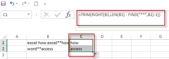
The find function will return the position of the first wildcard (**) character within a string in Cell B1. you need subtract the numeric position returned by FIND function from the length of the string in Cell B1 to get the length of sub string to the right of the wildcard character(asterisk). then the RIGHT function extracts the rightmost characters based on the length of sub string.
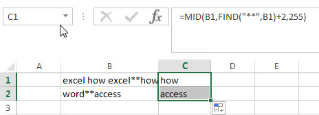
or you can use another formula to achieve the same result as follows:
=MID(B1,FIND("**",B1)+2,255)
Question 3: I am trying to extract the first word from another text string separated by space character. but it always return a #VALUE error message. I think it should be use the FIND function in combination with another function, such as: left function. but I still don’t know how to combine with those two functions to extract the first word.
Answer: right, you can create a excel formula that uses the FIND function and LEFT function. and you can use the below formula:
=IFERROR(LEFT(B1, FIND(" ",B1)-1),B1)
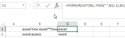
The find function returns the position of the first space character in the text string in Cell B1. the Formula “=FIND(” “,B1)-1 returns the numbers of the first word as the second arguments of the LEFT function.
If the text string in Cell B1 just only contains one word, then the find function will return #VALUE error. to handle this error, you need to use the IFERROR function, if the find function is not find the space character, then return the text string in B1. in other words, it just contains only one word in Cell B1.
Question 4: I am trying to extract an email address from a text string in Cell B1. how to write a excel formula to achieve the result.
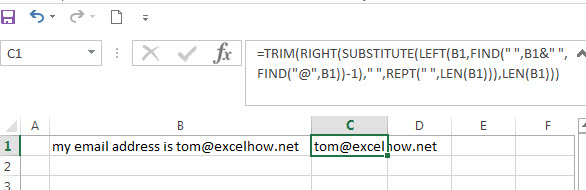
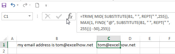
Answer: you can use a combination of the TRIM function, the LEFT function, the SUBSTITUTE function, the MID function, the MAX function and the REPT function to create a complex excel formula to extract email address from a string in Cell B1.
=TRIM(RIGHT(SUBSTITUTE(LEFT(B1,FIND (" ",B1&" ",FIND("@",B1))-1)," ", REPT(" ",LEN(B1))),LEN(B1)))
=TRIM( MID( SUBSTITUTE(B1, " ", REPT(" ",255)), MAX(1, FIND( "@", SUBSTITUTE(B1, " ", REPT(" ",255))) -50),255))
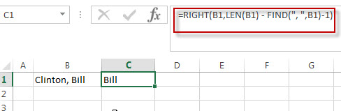
Question 5: I am trying to get the first name from a full name separated by a comma character. how to use a excel formula to extract the first name from a name as: “Last name, First name” format.
Answer: you can use a combination with the RIGHT function, the LEN function and the FIND function to create a excel formula to get the first name from a name. just using the following formula:
=RIGHT(B1,LEN(B1) - FIND(", ",B1)-1)
- Excel SEARCH function
The Excel SEARCH function returns the number of the starting location of a substring in a text string.The syntax of the SEARCH function is as below:= SEARCH (find_text, within_text,[start_num])… - Excel Find function
The Excel FIND function returns the position of the first text string (substring) from the first character of the second text string.The FIND function is a build-in function in Microsoft Excel and it is categorized as a Text Function.The syntax of the FIND function is as below:= FIND (find_text, within_text,[start_num])… - Excel ISERROR function
The Excel ISERROR function returns TRUE if the value is any error value except #N/A. The ISERROR function is a build-in function in Microsoft Excel and it is categorized as an Information Function. The syntax of the ISERROR function is as below: = ISERROR (value) … - Excel ISNUMBER function
The Excel ISNUMBER function returns TRUE if the value in a cell is a numeric value, otherwise it will return FALSE.The syntax of the ISNUMBER function is as below:= ISNUMBER (value)… - Excel RIGHT function
The Excel RIGHT function returns a sub string (a specified number of the characters) from a text string, starting from the rightmost character.The syntax of the RIGHT function is as below:= RIGHT (text,[num_chars])… - Excel LEN function
The Excel LEN function returns the length of a text string (the number of characters in a text string).The LEN function is a build-in function in Microsoft Excel and it is categorized as a Text Function.The syntax of the LEN function is as below:= LEN(text)… - Excel MID function
The Excel MID function returns a sub string from a text string at the position that you specify. The MID function is a build-in function in Microsoft Excel and it is categorized as a Text Function. The syntax of the MID function is as below: = MID (text, start_num, num_chars) … - Excel SUBSTITUTE function
The Excel SUBSTITUTE function replaces a new text string for an old text string in a text string.The syntax of the SUBSTITUTE function is as below:= SUBSTITUTE (text, old_text, new_text,[instance_num])… - Excel LEFT function
The Excel LEFT function returns a sub string (a specified number of the characters) from a text string, starting from the leftmost character.The LEFT function is a build-in function in Microsoft Excel and it is categorized as a Text Function.The syntax of the LEFT function is as below:= LEFT(text,[num_chars])… - Excel REPT function
The Excel REPT function repeats a text string a specified number of times.The REPT function is a build-in function in Microsoft Excel and it is categorized as a Text Function.The syntax of the REPT function is as below:= REPT (text, number_times)…
More FIND Formula Examples in Excel
-
Split Text String by Specified Character
you should use the Left function in combination with FIND function to split the text string in excel. And we can refer to the below formula that will find the position of “-“in Cell B1 and extract all the characters to the left of the dash character “-“.=LEFT(B1,FIND(“-“,B1,1)-1).… - Split Text String by Line Break
When you want to split text string by line break in excel, you should use a combination of the LEFT, RIGHT, CHAR, LEN and FIND functions. The CHAR (10) function will return the line break character, the FIND function will use the returned value of the CHAR function as the first argument to locate the position of the line break character within the cell B1.… - Split Text and Numbers in Excel
If you want to split text and numbers, you can run the following excel formula that use the MIN function, FIND function and the LEN function within the LEFT function in excel. .… - Get the Current Worksheet Name only
If you want to get the current worksheet name only in excel, you can use a combination of the MID function, the CELL function and FIND function.… - Get full File Name (workbook and worksheet) and Path
In excel, you can get the current workbook name and it is absolute path using the CELL function. Just refer to the following formula:=CELL(“filename”,B1).… - Get the Current Workbook Name
If you want to get the name of the current workbook only, you can use a combination of the MID function, the CELL function and the FIND Function… - Get Path and Workbook name only
If you want to get the workbook name and its path only without worksheet name, you can use a combination of the SUBSTITUTE function, the LEFT function, the CELL function and the FIND function…. - Get First Name From Full Name
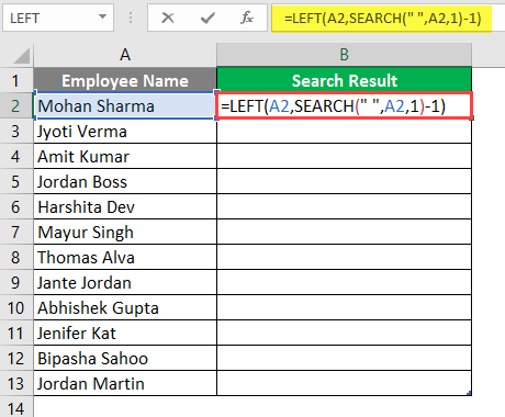
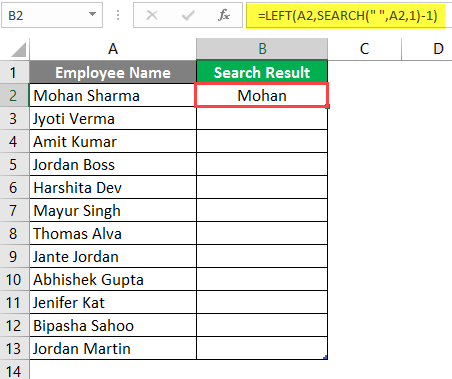
If you want to get the first name from a full name list in Column B, you can use the FIND function within LEFT function in excel. The generic formula is as follows:=LEFT(B1,FIND(” “,B1)-1).… - Get Last Name From Full Name
To extract the last name within a Full name in excel. You need to use a combination of the RIGHT function, the LEN function, the FIND function and the SUBSTITUTE function to create a complex formula in excel..… - The different between FIND and SEARCH functions
There are two big differences between FIND and SEARCH functions in excel.The FIND function is case-sensitive. And the SEARCH function is case-insensitive…… - Data Validation for Specified Text only
If you want to check if the values that contain a specified text string in one cell, you can use a combination of the FIND function and ISNUMBER function as a formula in the Data Validation….… - Count Cells That Contain Specific Text
This post will discuss that how to count the number of cells that contain specific text or certain text in a specified cells of range in Excel. How to get the total number of cells that contain certain text.…… - Split Text and Numbers
If you want to split text and numbers from one cell into two different cells, you can use a formula based on the FIND function, the LEFT function or the RIGHT function and the MIN function. .… - Quickly Get Sheet Name
If you want to quickly get current worksheet name only, then inert it into one cell. You can use a formula based on the MID function in combination with the FIND function and the Cell function…… - Sorting IP Address
Assuming that you have an IP list of data in the range of cells B1:B5, and you want to sort those IP list from low to high, how to achieve the result with excel formula. You need to create a formula based on the Text Function, the LEFT function, the FIND function and the MID function, the RIGHT function..… - Removing Salutation from Name
To remove salutation from names string in excel, you can create a formula based on the RIGHT function, the LEN function and the FIND function…… - List all Worksheet Names
Assuming that you have a workbook that has hundreds of worksheets and you want to get a list of all the worksheet names in the current workbook. And the below will introduce 3 methods with you..… - Insert The File Path and Filename into Cell
If you want to insert a file path and filename into a cell in your current worksheet, you can use the CELL function to create a formual……..
Many a time, it may have happened with you that you have a lot many formulas in your excel worksheet and you want to find only those cells that contain formulas. One way is to go to each and every cell one by one and then check if it contains any formula or not. But don’t you think that it is a quite time-consuming and irritating activity? Yes, it is. Indeed, there are many easy ways that you can use to find the cells containing formula at one click. In this blog, we would unlock this technique to find formula cells in Excel. There are multiple ways to achieve it.
As mentioned in the introduction paragraph of this blog, there are mainly three ways to find all the cells that contain formula in it. Let me list those down first.
Table of Contents
- Methods to Find Formula Cells
- Sample Example Data
- Find Formula Cells Using ISFORMULA function in Excel
- Using Conditional Formatting to Find Formula Cells
- Using GoTo Special Functionality
- Using the ISFORMULA function
- Using ‘Conditional Formatting’ Feature
- ‘GoTo Special’ Functionality
Sample Example Data
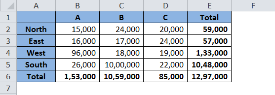
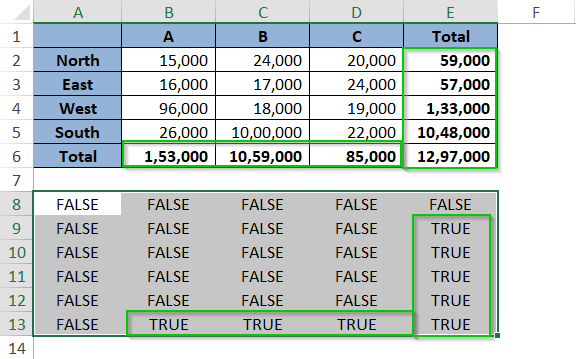
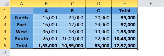
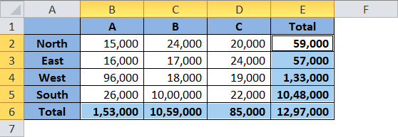
Below is the screenshot of containing sales data in a table format region wise. In this dataset, there are few cells that contain formula in it. The goal here is to find all the cell containing the formula.
Let us now start learning each of the methods one by one.
Find Formula Cells Using ISFORMULA function in Excel
In this method, we would learn how to use an excel pre-provided formula to find all the cells containing a formula in it. The formula about which I am talking about is – ‘ISFORMULA‘.
The formula nomenclature itself makes it clear that this function/formula would check if it IS a FORMULA.
Syntax and Attributes: The formula syntax goes like this: =ISFORMULA(reference); where ‘Reference’ means the reference of the cell or range.
Return Values: This formula returns ‘TRUE‘ if the reference cell contains a formula and ‘FALSE‘ in vice versa situation.
Let us now use this function in our example. Follow the below steps:
Select the exact number of cell range as that of the original data table somewhere in the worksheet. In my example, since I have the data table with 6 rows and 5 columns, therefore, I have selected exactly 6 rows and 5 columns at some other place in Excel (A5:E13). Refer to the screenshot below:
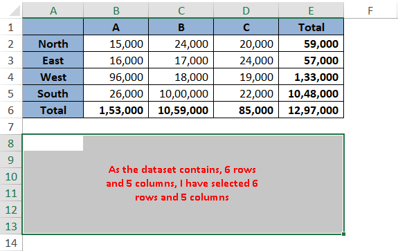
Make sure that the starting cell of the selection should be the top-left cell (in our example it is A8). As can be seen from the screenshot above, we started the selection from cell A8 and therefore, cell A8 is the active cell now.
Now, just type the formula =ISFORMULA(A1) and press Ctrl+Enter. As a result, you would notice that Excel enters the same formula in all the cells in the selected cell range.
Consequently, the formula returns TRUE and FALSE as a return value. This depicts that the reference cells corresponding to the cells with TRUE contain a formula. And the reference cells corresponding to the cells with FLASE do not contain any formula.
Using Conditional Formatting to Find Formula Cells
This method is an extension of the above method. One of the limitations of the above method is that the method does not provide the required information (that whether a cell contains a formula) in the cell itself. As you can see, the information that the cell E4 has a formula in it is provided in the cell E11 (as the return value TRUE).
To mitigate this, we can use the conditional formatting functionality along with the ISFORMULA function to find determine a formula cell (in that cell itself). Follow the procedure below:
Firstly, select the cell range (A1 to E6).
Now, navigate to the ‘Home’ tab. There you would find an option called ‘Conditional Formatting’.
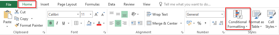
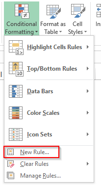
Click on this feature, and select the option ‘New Rule’ from the list of a drop-down menu.
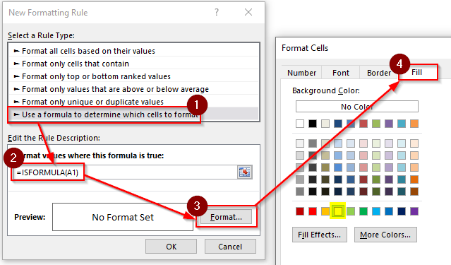
Under the ‘Select a Rule Type’ section, click on the last option ‘Use a formula to determine which cell to format’ and enter the formula =ISFORMULA(A1) in the input box available.
Next, click on the option ‘Format’ to open the ‘Format Cells’ dialog box. Under the tab named ‘Fill’, and select the cell fill color of your choice from the list of available colors (I have selected the Yellow color).
Finally, click on the ‘OK’ button to activate the format cell and then exit the ‘Conditional Formatting’ dialog box by clicking on the ‘OK’ button.
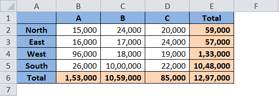
As a result, you would notice that the excel highlights all those cells that have a formula in it.
Using GoTo Special Functionality
This is yet another method to find all the cells containing the formula. This is a widely used method among all the other methods as no formula is needed to use this function. Follow the undermentioned steps-
Firstly, select the dataset table
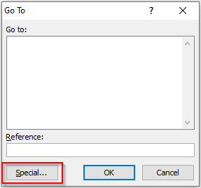
Now press Ctrl+G key combinations on your keyboard to open the “GoTo” dialog box.
In the “GoTo” dialog box, click on the “Special” option as highlighted in the screenshot below.
The “GoTo Special” dialog box would open.
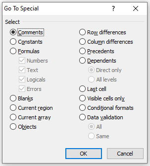
From the list of available options, click on the radio button “Formulas” and then click on the “OK” button to exit this dialog box.
As a result, you would notice that all the formula cells get selected.
Finally, just change the fill color of all those cells by choosing the color of your choice from the list of available colors. Refer to the screenshot below
You can even do any kind of formatting to these cells, like changing the font size, color, etc.
This brings us to the end of this blog. Share your views and comments in the comment section below.
RELATED POSTS
-
ISNUMBER Function of Excel – Checking If Cell Contains a Number
-
ISNONTEXT Function of Excel – Check Non Text Cell in Excel
-
Using =IF() Function For Partial Match in Excel
-
ISLOGICAL Function in Excel – Checking for Boolean TRUE/FALSE
-
How to Select Cells Containing Data Validation
-
SEARCH Function in Excel – Search String in Excel
Search Formula in Excel (Table of Contents)
- SEARCH Formula in Excel
- How to Use SEARCH Formula in Excel?
Search Formula in Excel
- The search Function is one of the most important in-built functions of MS Excel. It is used to locate or find one string in the second string; in simple words, it will locate a search text in the string. The Search function allows the wildcards (like: ??, *, ~), and it is not case-sensitive.
- For example, if there is a first-string “base” and a second string is the “database”, then the search function will return as 5, starting from the fifth letter in the second string.
Search Formula Syntax in Excel
SEARCH ()– It will return an integer value, which represents the position of the search string in the second string. There is three-parameter – find_text, within_text, [start_num].
The Argument in the SEARCH Function
- find_text: It is a mandatory parameter, the string which the user wants to SEARCH.
- within_text: It is a mandatory parameter, the string in which the user wants to SEARCH.
- find_text: It is an optional parameter, the character number from where the user wants to search in the within_text.
How to Use SEARCH Formula in Excel?
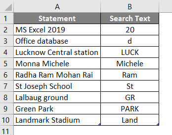
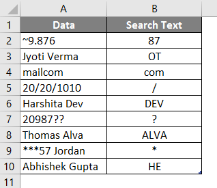
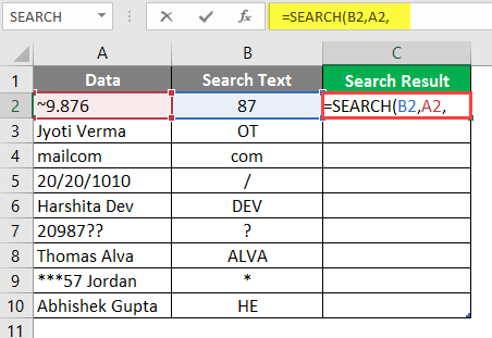
There is some statement given in the table and a search string also given which a user wants to search from the given statement. Let’s see how the SEARCH function can solve this problem.
You can download this SEARCH Formula Excel Template here – SEARCH Formula Excel Template
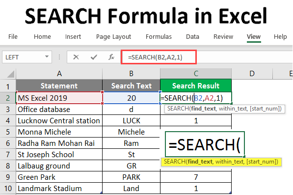
Example #1 – Use SEARCH Formula in Text
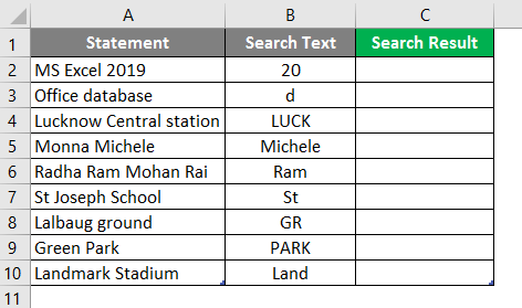
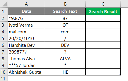
Open MS Excel, Go to Sheet1 where the user wants to SEARCH the text.
Create one column header for the SEARCH result to show the function result in the C column.
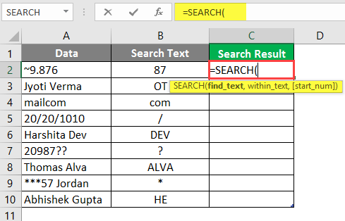
Click on the C2 cell and apply the SEARCH Formula.
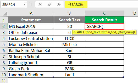
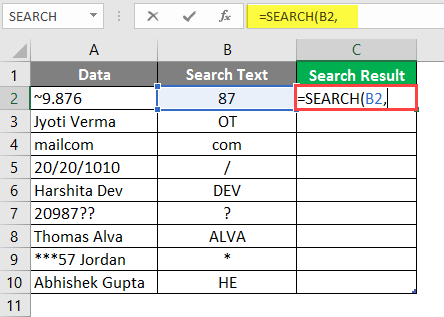
Now it will ask for find text; select the Search Text to search, which is available in B2.
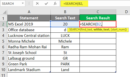
Now it will ask for within the Text, from where the user wants to search text which available in B2 cell.
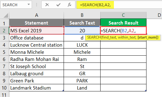
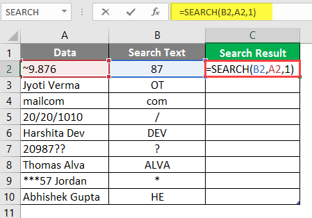
It will now ask for start Num, which by default value is 1, so we will give 1>> write in the C2 cell.
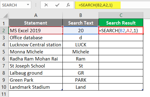
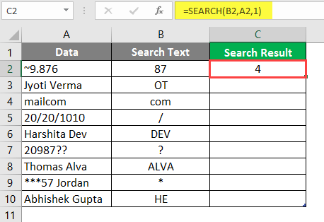
Press the Enter key.
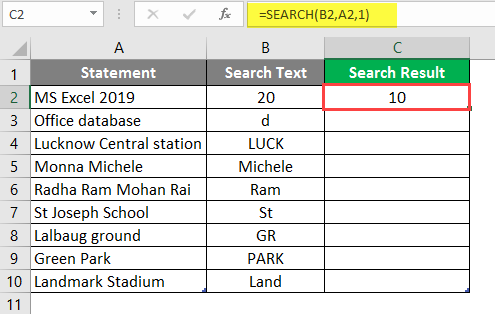
Drag the same formula to the other cell of the C column to find out the SEARCH Result.
Summary of Example 1:
As the user wants to SEARCH text in the given statement, the same can achieve by the search function. Which is available in column C as the search result.
Example #2 – Use the SEARCH Function for Wildcards
There is some data given that have wildcards (like: ??, *, ~) in the table, and a search string is also given that a user wants to search from the given data.
Let’s see how the SEARCH function can solve this problem.
Open MS Excel, Go to Sheet2 where the user wants to SEARCH the text.
Create one column header for the SEARCH result to show the function result in the C column.
Click on the C2 cell and apply the SEARCH Formula.
Now it will ask for find text; select the Search Text to search, which is available in B2.
It will now ask for within Text, from where the user wants to search text that is available in cell B2.
It will now ask for start Num, which by default value is 1, so we will give 1 >> write in the C2 cell.
Press on the Enter key.
Drag the same formula to the other cell of the C column to find out the SEARCH result.
Summary of Example 2:
As the user wants to SEARCH text in the given data, the same can achieve by the search function. Which is available in the C column as the search result.
Example #3 – Use the SEARCH Function with the help of the LEFT Function
There are some company employee details given in a table from where a user wants to get the first name of all employees.
Open MS Excel; go to Sheet 3, where the user wants to get the first name of all employees.
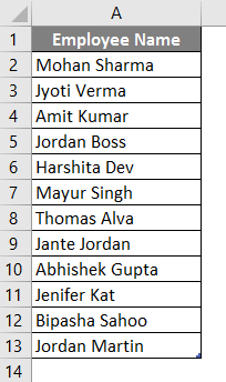
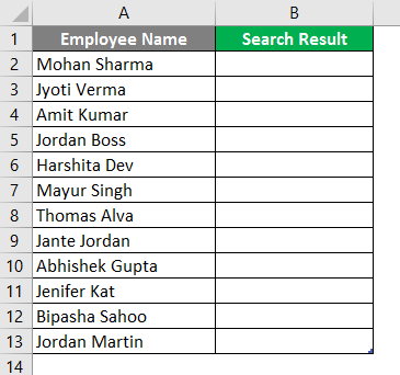
Create one column header for the SEARCH Result to show the function result in the B column.
Click on cell B2 and apply the first Left formula.
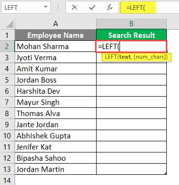
Now select cell B2, where the LEFT Formula will be applied.
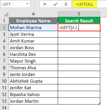
Now apply the SEARCH Formula.
Now it will ask for find text; the user will search for the first gap.
Now it will ask for within Text, from where the user wants to employees the first name which is available in the A2 cell.
It will now ask for start Num, which is by default value is 1, so we will give 1 >> write in B2 cell.
Now it will ask for num_char, which is the result of the search function >> Here space also counts as one character so need to minus 1 from the search function result.
Press on the Enter key.
Drag the same formula to the other cell of the B column to find out the SEARCH Result.
Summary of Example 3:
As the user wants to find out the first name of the employee. Same he has achieved by left and search function, which is available in the D column as the search result.
Things to Remember About Search Formula in Excel
- The Search function will return an integer value. A user can use this function with other formulas and functions.
- The Search function allows wildcards (like: ??, *, ~), and it is not case-sensitive. If a user wants to search for case-sensitive, then use the FIND function.
- If there is no matching for find_search in within_serach, then it will throw a #VALUE! Error.
- If start_num is greater than the length of the within_serach string or not greater than zero, then it will return a #VALUE! Error.
Recommended Articles
This has been a guide to Search formulas in Excel. Here we discuss How to Use Search Formulas in Excel along with practical examples and a downloadable Excel template. You can also go through our other suggested articles –
- Excel SEARCH Function
- Excel Search Box
- Search For Text in Excel
- Basic Excel Formulas