
Summary
This step-by-step article describes how to find data in a table (or range of cells) by using various built-in functions in Microsoft Excel. You can use different formulas to get the same result.
Create the Sample Worksheet
This article uses a sample worksheet to illustrate Excel built-in functions. Consider the example of referencing a name from column A and returning the age of that person from column C. To create this worksheet, enter the following data into a blank Excel worksheet.
You will type the value that you want to find into cell E2. You can type the formula in any blank cell in the same worksheet.
|
A |
B |
C |
D |
E |
||
|
1 |
Name |
Dept |
Age |
Find Value |
||
|
2 |
Henry |
501 |
28 |
Mary |
||
|
3 |
Stan |
201 |
19 |
|||
|
4 |
Mary |
101 |
22 |
|||
|
5 |
Larry |
301 |
29 |
Term Definitions
This article uses the following terms to describe the Excel built-in functions:
|
Term |
Definition |
Example |
|
Table Array |
The whole lookup table |
A2:C5 |
|
Lookup_Value |
The value to be found in the first column of Table_Array. |
E2 |
|
Lookup_Array |
The range of cells that contains possible lookup values. |
A2:A5 |
|
Col_Index_Num |
The column number in Table_Array the matching value should be returned for. |
3 (third column in Table_Array) |
|
Result_Array |
A range that contains only one row or column. It must be the same size as Lookup_Array or Lookup_Vector. |
C2:C5 |
|
Range_Lookup |
A logical value (TRUE or FALSE). If TRUE or omitted, an approximate match is returned. If FALSE, it will look for an exact match. |
FALSE |
|
Top_cell |
This is the reference from which you want to base the offset. Top_Cell must refer to a cell or range of adjacent cells. Otherwise, OFFSET returns the #VALUE! error value. |
|
|
Offset_Col |
This is the number of columns, to the left or right, that you want the upper-left cell of the result to refer to. For example, «5» as the Offset_Col argument specifies that the upper-left cell in the reference is five columns to the right of reference. Offset_Col can be positive (which means to the right of the starting reference) or negative (which means to the left of the starting reference). |
Functions
LOOKUP()
The LOOKUP function finds a value in a single row or column and matches it with a value in the same position in a different row or column.
The following is an example of LOOKUP formula syntax:
=LOOKUP(Lookup_Value,Lookup_Vector,Result_Vector)
The following formula finds Mary’s age in the sample worksheet:
=LOOKUP(E2,A2:A5,C2:C5)
The formula uses the value «Mary» in cell E2 and finds «Mary» in the lookup vector (column A). The formula then matches the value in the same row in the result vector (column C). Because «Mary» is in row 4, LOOKUP returns the value from row 4 in column C (22).
NOTE: The LOOKUP function requires that the table be sorted.
For more information about the LOOKUP function, click the following article number to view the article in the Microsoft Knowledge Base:
How to use the LOOKUP function in Excel
VLOOKUP()
The VLOOKUP or Vertical Lookup function is used when data is listed in columns. This function searches for a value in the left-most column and matches it with data in a specified column in the same row. You can use VLOOKUP to find data in a sorted or unsorted table. The following example uses a table with unsorted data.
The following is an example of VLOOKUP formula syntax:
=VLOOKUP(Lookup_Value,Table_Array,Col_Index_Num,Range_Lookup)
The following formula finds Mary’s age in the sample worksheet:
=VLOOKUP(E2,A2:C5,3,FALSE)
The formula uses the value «Mary» in cell E2 and finds «Mary» in the left-most column (column A). The formula then matches the value in the same row in Column_Index. This example uses «3» as the Column_Index (column C). Because «Mary» is in row 4, VLOOKUP returns the value from row 4 in column C (22).
For more information about the VLOOKUP function, click the following article number to view the article in the Microsoft Knowledge Base:
How to Use VLOOKUP or HLOOKUP to find an exact match
INDEX() and MATCH()
You can use the INDEX and MATCH functions together to get the same results as using LOOKUP or VLOOKUP.
The following is an example of the syntax that combines INDEX and MATCH to produce the same results as LOOKUP and VLOOKUP in the previous examples:
=INDEX(Table_Array,MATCH(Lookup_Value,Lookup_Array,0),Col_Index_Num)
The following formula finds Mary’s age in the sample worksheet:
=INDEX(A2:C5,MATCH(E2,A2:A5,0),3)
The formula uses the value «Mary» in cell E2 and finds «Mary» in column A. It then matches the value in the same row in column C. Because «Mary» is in row 4, the formula returns the value from row 4 in column C (22).
NOTE: If none of the cells in Lookup_Array match Lookup_Value («Mary»), this formula will return #N/A.
For more information about the INDEX function, click the following article number to view the article in the Microsoft Knowledge Base:
How to use the INDEX function to find data in a table
OFFSET() and MATCH()
You can use the OFFSET and MATCH functions together to produce the same results as the functions in the previous example.
The following is an example of syntax that combines OFFSET and MATCH to produce the same results as LOOKUP and VLOOKUP:
=OFFSET(top_cell,MATCH(Lookup_Value,Lookup_Array,0),Offset_Col)
This formula finds Mary’s age in the sample worksheet:
=OFFSET(A1,MATCH(E2,A2:A5,0),2)
The formula uses the value «Mary» in cell E2 and finds «Mary» in column A. The formula then matches the value in the same row but two columns to the right (column C). Because «Mary» is in column A, the formula returns the value in row 4 in column C (22).
For more information about the OFFSET function, click the following article number to view the article in the Microsoft Knowledge Base:
How to use the OFFSET function
Need more help?
Функция НАЙТИ (FIND) в Excel используется для поиска текстового значения внутри строчки с текстом и указать порядковый номер буквы с которого начинается искомое слово в найденной строке.
Содержание
- Что возвращает функция
- Синтаксис
- Аргументы функции
- Дополнительная информация
- Примеры использования функции НАЙТИ в Excel
- Пример 1. Ищем слово в текстовой строке (с начала строки)
- Пример 2. Ищем слово в текстовой строке (с заданным порядковым номером старта поиска)
- Пример 3. Поиск текстового значения внутри текстовой строки с дублированным искомым значением
Что возвращает функция
Возвращает числовое значение, обозначающее стартовую позицию текстовой строчки внутри другой текстовой строчки.
Синтаксис
=FIND(find_text, within_text, [start_num]) — английская версия
=НАЙТИ(искомый_текст;просматриваемый_текст;[нач_позиция]) — русская версия
Аргументы функции
- find_text (искомый_текст) — текст или строка которую вы хотите найти в рамках другой строки;
- within_text (просматриваемый_текст) — текст, внутри которого вы хотите найти аргумент find_text (искомый_текст);
- [start_num] ([нач_позиция]) — число, отображающее позицию, с которой вы хотите начать поиск. Если аргумент не указать, то поиск начнется сначала.
Дополнительная информация
- Если стартовое число не указано, то функция начинает поиск искомого текста с начала строки;
- Функция НАЙТИ чувствительна к регистру. Если вы хотите сделать поиск без учета регистра, используйте функцию SEARCH в Excel;
- Функция не учитывает подстановочные знаки при поиске. Если вы хотите использовать подстановочные знаки для поиска, используйте функцию SEARCH в Excel;
- Функция каждый раз возвращает ошибку, когда не находит искомый текст в заданной строке.
Примеры использования функции НАЙТИ в Excel
Пример 1. Ищем слово в текстовой строке (с начала строки)

На примере выше мы ищем слово «Доброе» в словосочетании «Доброе Утро». По результатам поиска, функция выдает число «1», которое обозначает, что слово «Доброе» начинается с первой по очереди буквы в, заданной в качестве области поиска, текстовой строке.
Больше лайфхаков в нашем Telegram Подписаться
Обратите внимание, что так как функция НАЙТИ в Excel чувствительна к регистру, вы не сможете найти слово «доброе» в словосочетании «Доброе утро», так как оно написано с маленькой буквы. Для того, чтобы осуществить поиска без учета регистра следует пользоваться функцией SEARCH.
Пример 2. Ищем слово в текстовой строке (с заданным порядковым номером старта поиска)
Третий аргумент функции НАЙТИ указывает позицию, с которой функция начинает поиск искомого значения. На примере выше функция возвращает число «1» когда мы начинаем поиск слова «Доброе» в словосочетании «Доброе утро» с начала текстовой строки. Но если мы зададим аргумент функции start_num (нач_позиция) со значением «2», то функция выдаст ошибку, так как начиная поиск со второй буквы текстовой строки, она не может ничего найти.
Если вы не укажете номер позиции, с которой функции следует начинать поиск искомого аргумента, то Excel по умолчанию начнет поиск с самого начала текстовой строки.
Пример 3. Поиск текстового значения внутри текстовой строки с дублированным искомым значением
На примере выше мы ищем слово «Доброе» в словосочетании «Доброе Доброе утро». Когда мы начинаем поиск слова «Доброе» с начала текстовой строки, то функция выдает число «1», так как первое слово «Доброе» начинается с первой буквы в словосочетании «Доброе Доброе утро».
Но, если мы укажем в качестве аргумента start_num (нач_позиция) число «2» и попросим функцию начать поиск со второй буквы в заданной текстовой строке, то функция выдаст число «6», так как Excel находит искомое слово «Доброе» начиная со второй буквы словосочетания «Доброе Доброе утро» только на 6 позиции.
Содержание
- Поисковая функция в Excel
- Способ 1: простой поиск
- Способ 2: поиск по указанному интервалу ячеек
- Способ 3: Расширенный поиск
- Вопросы и ответы

В документах Microsoft Excel, которые состоят из большого количества полей, часто требуется найти определенные данные, наименование строки, и т.д. Очень неудобно, когда приходится просматривать огромное количество строк, чтобы найти нужное слово или выражение. Сэкономить время и нервы поможет встроенный поиск Microsoft Excel. Давайте разберемся, как он работает, и как им пользоваться.
Поисковая функция в Excel
Поисковая функция в программе Microsoft Excel предлагает возможность найти нужные текстовые или числовые значения через окно «Найти и заменить». Кроме того, в приложении имеется возможность расширенного поиска данных.
Способ 1: простой поиск
Простой поиск данных в программе Excel позволяет найти все ячейки, в которых содержится введенный в поисковое окно набор символов (буквы, цифры, слова, и т.д.) без учета регистра.
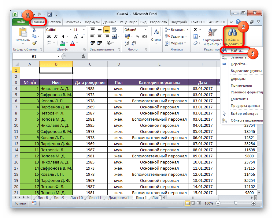
- Находясь во вкладке «Главная», кликаем по кнопке «Найти и выделить», которая расположена на ленте в блоке инструментов «Редактирование». В появившемся меню выбираем пункт «Найти…». Вместо этих действий можно просто набрать на клавиатуре сочетание клавиш Ctrl+F.
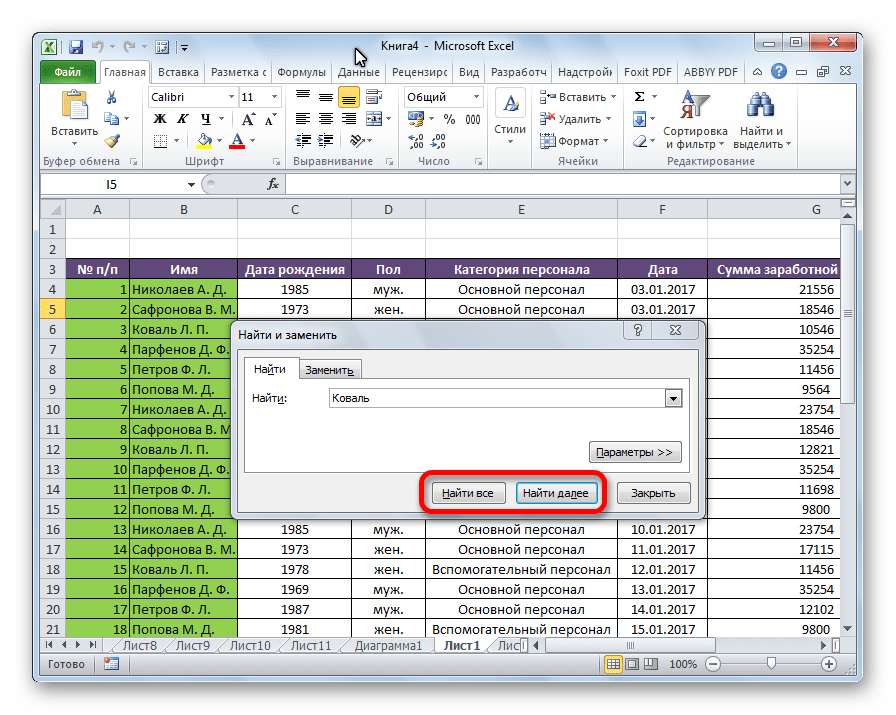
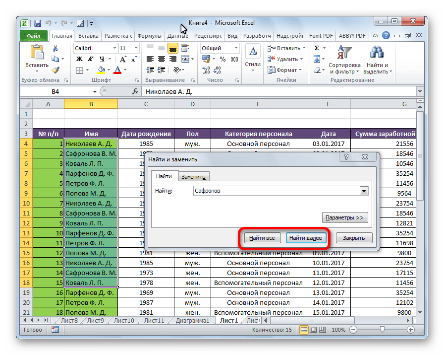
- После того, как вы перешли по соответствующим пунктам на ленте, или нажали комбинацию «горячих клавиш», откроется окно «Найти и заменить» во вкладке «Найти». Она нам и нужна. В поле «Найти» вводим слово, символы, или выражения, по которым собираемся производить поиск. Жмем на кнопку «Найти далее», или на кнопку «Найти всё».
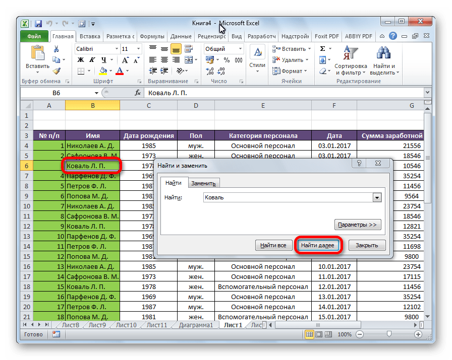
- При нажатии на кнопку «Найти далее» мы перемещаемся к первой же ячейке, где содержатся введенные группы символов. Сама ячейка становится активной.
Поиск и выдача результатов производится построчно. Сначала обрабатываются все ячейки первой строки. Если данные отвечающие условию найдены не были, программа начинает искать во второй строке, и так далее, пока не отыщет удовлетворительный результат.
Поисковые символы не обязательно должны быть самостоятельными элементами. Так, если в качестве запроса будет задано выражение «прав», то в выдаче будут представлены все ячейки, которые содержат данный последовательный набор символов даже внутри слова. Например, релевантным запросу в этом случае будет считаться слово «Направо». Если вы зададите в поисковике цифру «1», то в ответ попадут ячейки, которые содержат, например, число «516».
Для того, чтобы перейти к следующему результату, опять нажмите кнопку «Найти далее».

Так можно продолжать до тех, пор, пока отображение результатов не начнется по новому кругу.
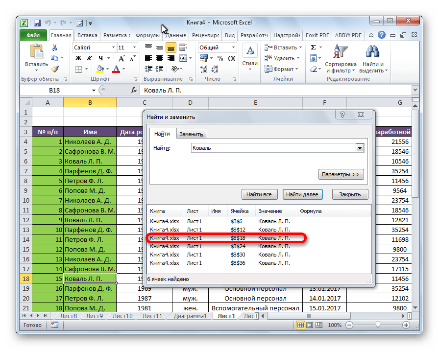
- В случае, если при запуске поисковой процедуры вы нажмете на кнопку «Найти все», все результаты выдачи будут представлены в виде списка в нижней части поискового окна. В этом списке находятся информация о содержимом ячеек с данными, удовлетворяющими запросу поиска, указан их адрес расположения, а также лист и книга, к которым они относятся. Для того, чтобы перейти к любому из результатов выдачи, достаточно просто кликнуть по нему левой кнопкой мыши. После этого курсор перейдет на ту ячейку Excel, по записи которой пользователь сделал щелчок.
Способ 2: поиск по указанному интервалу ячеек
Если у вас довольно масштабная таблица, то в таком случае не всегда удобно производить поиск по всему листу, ведь в поисковой выдаче может оказаться огромное количество результатов, которые в конкретном случае не нужны. Существует способ ограничить поисковое пространство только определенным диапазоном ячеек.
- Выделяем область ячеек, в которой хотим произвести поиск.
- Набираем на клавиатуре комбинацию клавиш Ctrl+F, после чего запуститься знакомое нам уже окно «Найти и заменить». Дальнейшие действия точно такие же, что и при предыдущем способе. Единственное отличие будет состоять в том, что поиск выполняется только в указанном интервале ячеек.
Способ 3: Расширенный поиск
Как уже говорилось выше, при обычном поиске в результаты выдачи попадают абсолютно все ячейки, содержащие последовательный набор поисковых символов в любом виде не зависимо от регистра.

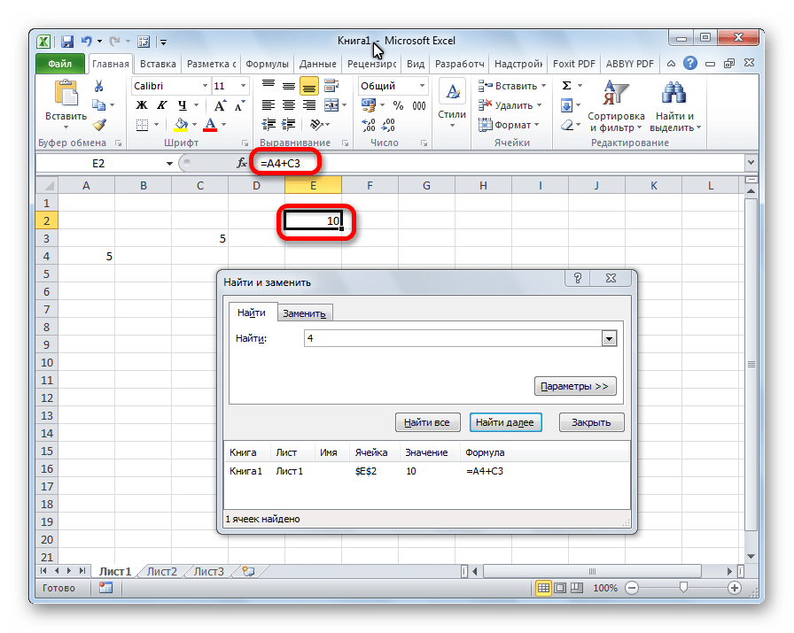
К тому же, в выдачу может попасть не только содержимое конкретной ячейки, но и адрес элемента, на который она ссылается. Например, в ячейке E2 содержится формула, которая представляет собой сумму ячеек A4 и C3. Эта сумма равна 10, и именно это число отображается в ячейке E2. Но, если мы зададим в поиске цифру «4», то среди результатов выдачи будет все та же ячейка E2. Как такое могло получиться? Просто в ячейке E2 в качестве формулы содержится адрес на ячейку A4, который как раз включает в себя искомую цифру 4.
Но, как отсечь такие, и другие заведомо неприемлемые результаты выдачи поиска? Именно для этих целей существует расширенный поиск Excel.
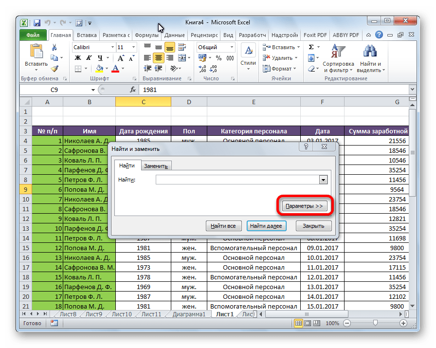
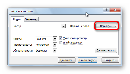
- После открытия окна «Найти и заменить» любым вышеописанным способом, жмем на кнопку «Параметры».
- В окне появляется целый ряд дополнительных инструментов для управления поиском. По умолчанию все эти инструменты находятся в состоянии, как при обычном поиске, но при необходимости можно выполнить корректировку.

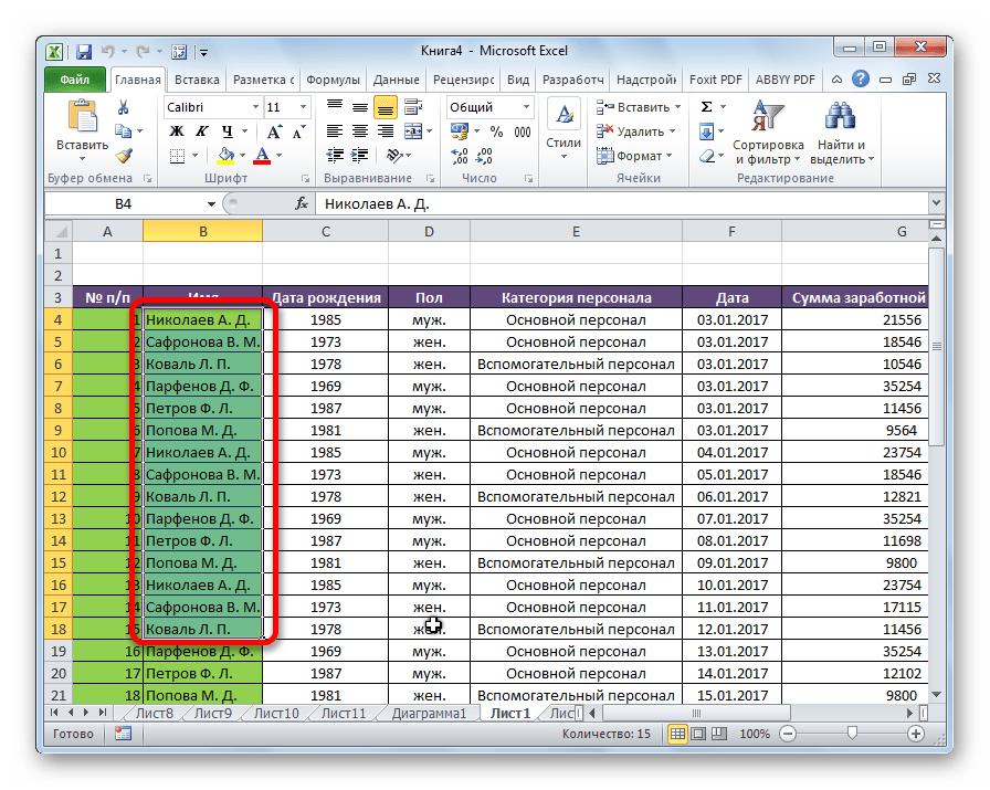
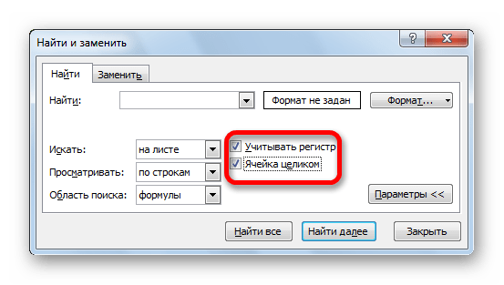
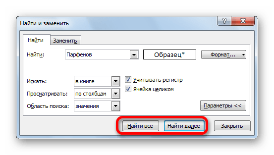
По умолчанию, функции «Учитывать регистр» и «Ячейки целиком» отключены, но, если мы поставим галочки около соответствующих пунктов, то в таком случае, при формировании результата будет учитываться введенный регистр, и точное совпадение. Если вы введете слово с маленькой буквы, то в поисковую выдачу, ячейки содержащие написание этого слова с большой буквы, как это было бы по умолчанию, уже не попадут. Кроме того, если включена функция «Ячейки целиком», то в выдачу будут добавляться только элементы, содержащие точное наименование. Например, если вы зададите поисковый запрос «Николаев», то ячейки, содержащие текст «Николаев А. Д.», в выдачу уже добавлены не будут.
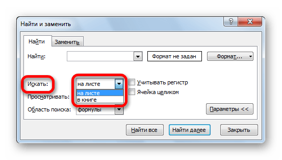
По умолчанию, поиск производится только на активном листе Excel. Но, если параметр «Искать» вы переведете в позицию «В книге», то поиск будет производиться по всем листам открытого файла.
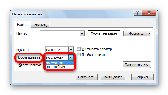
В параметре «Просматривать» можно изменить направление поиска. По умолчанию, как уже говорилось выше, поиск ведется по порядку построчно. Переставив переключатель в позицию «По столбцам», можно задать порядок формирования результатов выдачи, начиная с первого столбца.
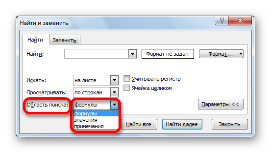
В графе «Область поиска» определяется, среди каких конкретно элементов производится поиск. По умолчанию, это формулы, то есть те данные, которые при клике по ячейке отображаются в строке формул. Это может быть слово, число или ссылка на ячейку. При этом, программа, выполняя поиск, видит только ссылку, а не результат. Об этом эффекте велась речь выше. Для того, чтобы производить поиск именно по результатам, по тем данным, которые отображаются в ячейке, а не в строке формул, нужно переставить переключатель из позиции «Формулы» в позицию «Значения». Кроме того, существует возможность поиска по примечаниям. В этом случае, переключатель переставляем в позицию «Примечания».
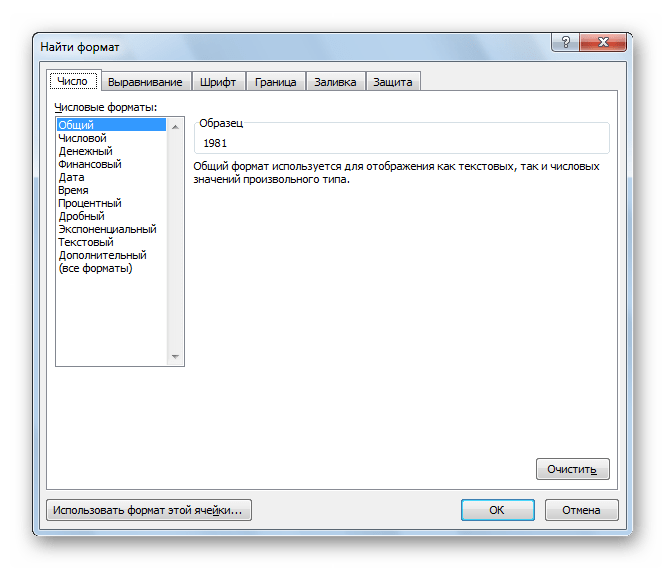
Ещё более точно поиск можно задать, нажав на кнопку «Формат».
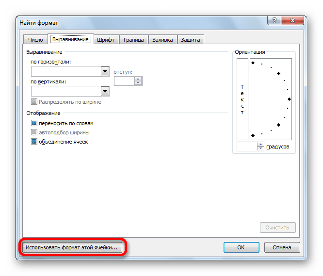
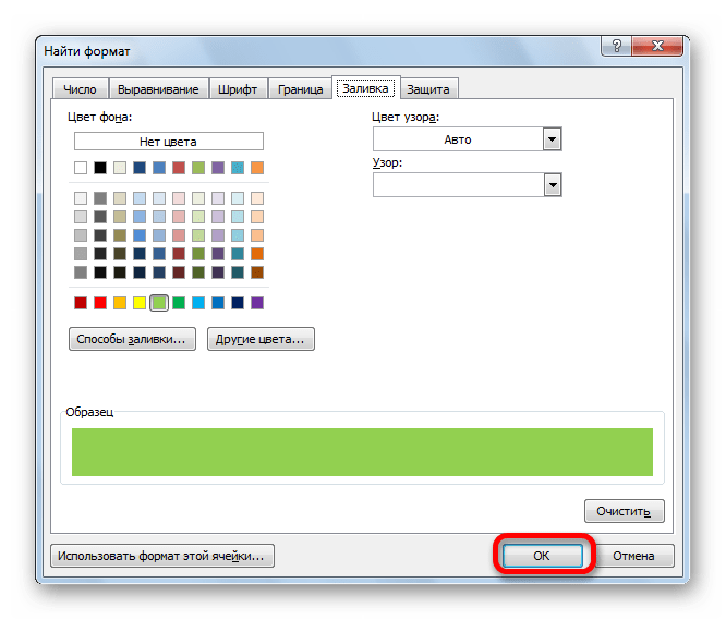
При этом открывается окно формата ячеек. Тут можно установить формат ячеек, которые будут участвовать в поиске. Можно устанавливать ограничения по числовому формату, по выравниванию, шрифту, границе, заливке и защите, по одному из этих параметров, или комбинируя их вместе.

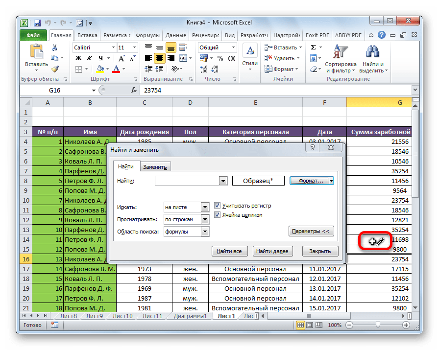
Если вы хотите использовать формат какой-то конкретной ячейки, то в нижней части окна нажмите на кнопку «Использовать формат этой ячейки…».
После этого, появляется инструмент в виде пипетки. С помощью него можно выделить ту ячейку, формат которой вы собираетесь использовать.
После того, как формат поиска настроен, жмем на кнопку «OK».
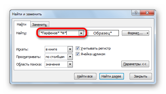
Бывают случаи, когда нужно произвести поиск не по конкретному словосочетанию, а найти ячейки, в которых находятся поисковые слова в любом порядке, даже, если их разделяют другие слова и символы. Тогда данные слова нужно выделить с обеих сторон знаком «*». Теперь в поисковой выдаче будут отображены все ячейки, в которых находятся данные слова в любом порядке.
- Как только настройки поиска установлены, следует нажать на кнопку «Найти всё» или «Найти далее», чтобы перейти к поисковой выдаче.

Как видим, программа Excel представляет собой довольно простой, но вместе с тем очень функциональный набор инструментов поиска. Для того, чтобы произвести простейший писк, достаточно вызвать поисковое окно, ввести в него запрос, и нажать на кнопку. Но, в то же время, существует возможность настройки индивидуального поиска с большим количеством различных параметров и дополнительных настроек.

Поиск какого-либо значения в ячейках Excel довольно часто встречающаяся задача при программировании какого-либо макроса. Решить ее можно разными способами. Однако, в разных ситуациях использование того или иного способа может быть не оправданным. В данной статье я рассмотрю 2 наиболее распространенных способа.
Поиск перебором значений
Довольно простой в реализации способ. Например, найти в колонке «A» ячейку, содержащую «123» можно примерно так:
Sheets("Данные").Select
For y = 1 To Cells.SpecialCells(xlLastCell).Row
    If Cells(y, 1) = "123" Then
        Exit For
    End If
Next y
MsgBox "Нашел в строке: " + CStr(y)
Минусами этого так сказать «классического» способа являются: медленная работа и громоздкость. А плюсом является его гибкость, т.к. таким способом можно реализовать сколь угодно сложные варианты поиска с различными вычислениями и т.п.
Поиск функцией Find
Гораздо быстрее обычного перебора и при этом довольно гибкий. В простейшем случае, чтобы найти в колонке A ячейку, содержащую «123» достаточно такого кода:
Sheets("Данные").Select
Set fcell = Columns("A:A").Find("123")
If Not fcell Is Nothing Then
    MsgBox "Нашел в строке: " + CStr(fcell.Row)
End If
Вкратце опишу что делают строчки данного кода:
1-я строка: Выбираем в книге лист «Данные»;
2-я строка: Осуществляем поиск значения «123» в колонке «A», результат поиска будет в fcell;
3-я строка: Если удалось найти значение, то fcell будет содержать Range-объект, в противном случае — будет пустой, т.е. Nothing.
Полностью синтаксис оператора поиска выглядит так:
Find(What, After, LookIn, LookAt, SearchOrder, SearchDirection, MatchCase, MatchByte, SearchFormat)
What — Строка с текстом, который ищем или любой другой тип данных Excel
After — Ячейка, после которой начать поиск. Обратите внимание, что это должна быть именно единичная ячейка, а не диапазон. Поиск начинается после этой ячейки, а не с нее. Поиск в этой ячейке произойдет только когда весь диапазон будет просмотрен и поиск начнется с начала диапазона и до этой ячейки включительно.
LookIn — Тип искомых данных. Может принимать одно из значений: xlFormulas (формулы), xlValues (значения), или xlNotes (примечания).
LookAt — Одно из значений: xlWhole (полное совпадение) или xlPart (частичное совпадение).
SearchOrder — Одно из значений: xlByRows (просматривать по строкам) или xlByColumns (просматривать по столбцам)
SearchDirection — Одно из значений: xlNext (поиск вперед) или xlPrevious (поиск назад)
MatchCase — Одно из значений: True (поиск чувствительный к регистру) или False (поиск без учета регистра)
MatchByte — Применяется при использовании мультибайтных кодировок: True (найденный мультибайтный символ должен соответствовать только мультибайтному символу) или False (найденный мультибайтный символ может соответствовать однобайтному символу)
SearchFormat — Используется вместе с FindFormat. Сначала задается значение FindFormat (например, для поиска ячеек с курсивным шрифтом так: Application.FindFormat.Font.Italic = True), а потом при использовании метода Find указываем параметр SearchFormat = True. Если при поиске не нужно учитывать формат ячеек, то нужно указать SearchFormat = False.
Чтобы продолжить поиск, можно использовать FindNext (искать «далее») или FindPrevious (искать «назад»).
Примеры поиска функцией Find
Пример 1: Найти в диапазоне «A1:A50» все ячейки с текстом «asd» и поменять их все на «qwe»
With Worksheets(1).Range("A1:A50")
  Set c = .Find("asd", LookIn:=xlValues)
  Do While Not c Is Nothing
    c.Value = "qwe"
    Set c = .FindNext(c)
  Loop
End With
Обратите внимание: Когда поиск достигнет конца диапазона, функция продолжит искать с начала диапазона. Таким образом, если значение найденной ячейки не менять, то приведенный выше пример зациклится в бесконечном цикле. Поэтому, чтобы этого избежать (зацикливания), можно сделать следующим образом:
Пример 2: Правильный поиск значения с использованием FindNext, не приводящий к зацикливанию.
With Worksheets(1).Range("A1:A50")
  Set c = .Find("asd", lookin:=xlValues)
  If Not c Is Nothing Then
    firstResult = c.Address
    Do
      c.Font.Bold = True
      Set c = .FindNext(c)
      If c Is Nothing Then Exit Do
    Loop While c.Address <> firstResult
  End If
End With
В ниже следующем примере используется другой вариант продолжения поиска — с помощью той же функции Find с параметром After. Когда найдена очередная ячейка, следующий поиск будет осуществляться уже после нее. Однако, как и с FindNext, когда будет достигнут конец диапазона, Find продолжит поиск с его начала, поэтому, чтобы не произошло зацикливания, необходимо проверять совпадение с первым результатом поиска.
Пример 3: Продолжение поиска с использованием Find с параметром After.
With Worksheets(1).Range("A1:A50")
  Set c = .Find("asd", lookin:=xlValues)
  If Not c Is Nothing Then
    firstResult = c.Address
    Do
      c.Font.Bold = True
      Set c = .Find("asd", After:=c, lookin:=xlValues)
      If c Is Nothing Then Exit Do
    Loop While c.Address <> firstResult
  End If
End With
Следующий пример демонстрирует применение SearchFormat для поиска по формату ячейки. Для указания формата необходимо задать свойство FindFormat.
Пример 4: Найти все ячейки с шрифтом «курсив» и поменять их формат на обычный (не «курсив»)
lLastRow = Cells.SpecialCells(xlLastCell).Row
lLastCol = Cells.SpecialCells(xlLastCell).Column
Application.FindFormat.Font.Italic = True
With Worksheets(1).Range(Cells(1, 1), Cells(lLastRow, lLastCol))
  Set c = .Find("", SearchFormat:=True)
  Do While Not c Is Nothing
    c.Font.Italic = False
    Set c = .Find("", After:=c, SearchFormat:=True)
  Loop
End With
Примечание: В данном примере намеренно не используется FindNext для поиска следующей ячейки, т.к. он не учитывает формат (статья об этом: https://support.microsoft.com/ru-ru/kb/282151)
Коротко опишу алгоритм поиска Примера 4. Первые две строки определяют последнюю строку (lLastRow) на листе и последний столбец (lLastCol). 3-я строка задает формат поиска, в данном случае, будем искать ячейки с шрифтом Italic. 4-я строка определяет область ячеек с которой будет работать программа (с ячейки A1 и до последней строки и последнего столбца). 5-я строка осуществляет поиск с использованием SearchFormat. 6-я строка — цикл пока результат поиска не будет пустым. 7-я строка — меняем шрифт на обычный (не курсив), 8-я строка продолжаем поиск после найденной ячейки.
Хочу обратить внимание на то, что в этом примере я не стал использовать «защиту от зацикливания», как в Примерах 2 и 3, т.к. шрифт меняется и после «прохождения» по всем ячейкам, больше не останется ни одной ячейки с курсивом.
Свойство FindFormat можно задавать разными способами, например, так:
With Application.FindFormat.Font
  .Name = "Arial"
  .FontStyle = "Regular"
  .Size = 10
End With
Поиск последней заполненной ячейки с помощью Find
Следующий пример — применение функции Find для поиска последней ячейки с заполненными данными. Использованные в Примере 4 SpecialCells находит последнюю ячейку даже если она не содержит ничего, но отформатирована или в ней раньше были данные, но были удалены.
Пример 5: Найти последнюю колонку и столбец, заполненные данными
Set c = Worksheets(1).UsedRange.Find("*", SearchDirection:=xlPrevious)
If Not c Is Nothing Then
  lLastRow = c.Row: lLastCol = c.Column
Else
  lLastRow = 1: lLastCol = 1
End If
MsgBox "lLastRow=" & lLastRow & " lLastCol=" & lLastCol
В этом примере используется UsedRange, который так же как и SpecialCells возвращает все используемые ячейки, в т.ч. и те, что были использованы ранее, а сейчас пустые. Функция Find ищет ячейку с любым значением с конца диапазона.
Поиск по шаблону (маске)
При поиске можно так же использовать шаблоны, чтобы найти текст по маске, следующий пример это демонстрирует.
Пример 6: Выделить красным шрифтом ячейки, в которых текст начинается со слова из 4-х букв, первая и последняя буквы «т», при этом после этого слова может следовать любой текст.
With Worksheets(1).Cells
  Set c = .Find("т??т*", LookIn:=xlValues, LookAt:=xlWhole)
  If Not c Is Nothing Then
    firstResult = c.Address
    Do
      c.Font.Color = RGB(255, 0, 0)
      Set c = .FindNext(c)
      If c Is Nothing Then Exit Do
    Loop While c.Address <> firstResult
  End If
End With
Для поиска функцией Find по маске (шаблону) можно применять символы:
* — для обозначения любого количества любых символов;
? — для обозначения одного любого символа;
~ — для обозначения символов *, ? и ~. (т.е. чтобы искать в тексте вопросительный знак, нужно написать ~?, чтобы искать именно звездочку (*), нужно написать ~* и наконец, чтобы найти в тексте тильду, необходимо написать ~~)
Поиск в скрытых строках и столбцах
Для поиска в скрытых ячейках нужно учитывать лишь один нюанс: поиск нужно осуществлять в формулах, а не в значениях, т.е. нужно использовать LookIn:=xlFormulas
Поиск даты с помощью Find
Если необходимо найти текущую дату или какую-то другую дату на листе Excel или в диапазоне с помощью Find, необходимо учитывать несколько нюансов:
- Тип данных Date в VBA представляется в виде #[месяц]/[день]/[год]#, соответственно, если необходимо найти фиксированную дату, например, 01 марта 2018 года, необходимо искать #3/1/2018#, а не «01.03.2018»
- В зависимости от формата ячеек, дата может выглядеть по-разному, поэтому, чтобы искать дату независимо от формата, поиск нужно делать не в значениях, а в формулах, т.е. использовать LookIn:=xlFormulas
Приведу несколько примеров поиска даты.
Пример 7: Найти текущую дату на листе независимо от формата отображения даты.
d = Date
Set c = Cells.Find(d, LookIn:=xlFormulas, LookAt:=xlWhole)
If Not c Is Nothing Then
  MsgBox "Нашел"
Else
  MsgBox "Не нашел"
End If
Пример 8: Найти 1 марта 2018 г.
d = #3/1/2018#
Set c = Cells.Find(d, LookIn:=xlFormulas, LookAt:=xlWhole)
If Not c Is Nothing Then
  MsgBox "Нашел"
Else
  MsgBox "Не нашел"
End If
Искать часть даты — сложнее. Например, чтобы найти все ячейки, где месяц «март», недостаточно искать «03» или «3». Не работает с датами так же и поиск по шаблону. Единственный вариант, который я нашел — это выбрать формат в котором месяц прописью для ячеек с датами и искать слово «март» в xlValues.
Тем не менее, можно найти, например, 1 марта независимо от года.
Пример 9: Найти 1 марта любого года.
d = #3/1/1900#
Set c = Cells.Find(Format(d, "m/d/"), LookIn:=xlFormulas, LookAt:=xlPart)
If Not c Is Nothing Then
  MsgBox "Нашел"
Else
  MsgBox "Не нашел"
End If
Find in Excel (Table of Contents)
- Using Find and Select Feature in Excel
- FIND Function in Excel
- SEARCH Function in Excel
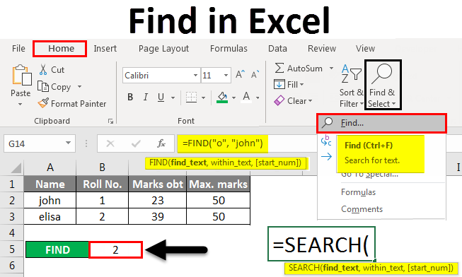
Introduction to Find in Excel
There are two ways to find it in Excel. First, we can use Find by pressing Ctrl + F shortcut keys. Therein Find and Replace box, search the word or field which we want to find in the Find What section. In another way, we can use the FIND function. For this, select the Find function from the insert function and, as per syntax, select the substring from where we need to find it, and choose the word or letter or number which we want to find in the String position. This will return the position of the chosen string from the selected Substring.
Methods to Find in Excel
Below are the different methods to find in excel.
You can download this Find in Excel Template here – Find in Excel Template
Method #1 – Using Find and Select Feature in Excel
Let’s see How to Find a Number or a Character in Excel using the Find and Select feature in Excel.
Step 1 – Under the Home tab, in the Editing group, click Find & Select.
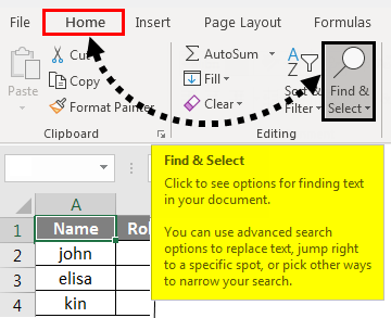
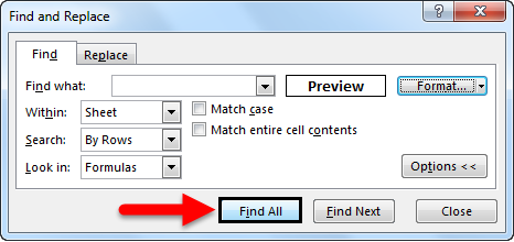
Step 2 – To find text or numbers, click Find.
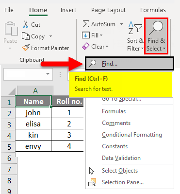
- In the Find what box, type the text or character you want to search for, or click the arrow in the Find what box and then click a recent search in the list.
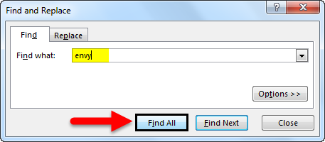
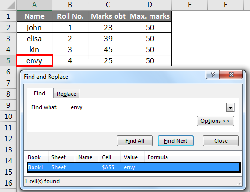
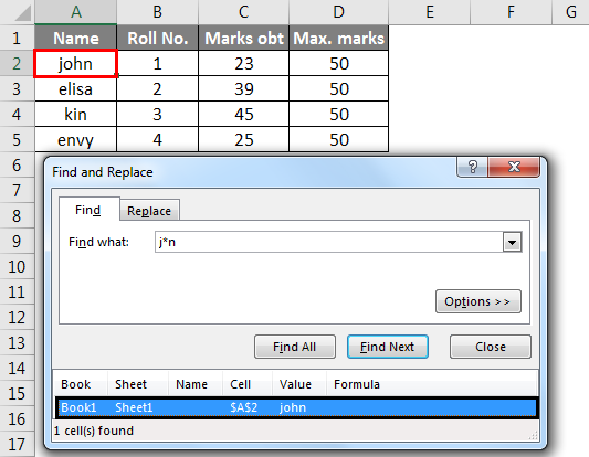
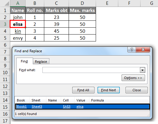
Here, we have a record of marks of four students. Suppose we want to find the text ‘envy’ in this table. For this, we click Find and Select under the Home tab then the Find and Replace dialog box appears. In the Find what box, we enter ‘envy’ then click on Find All. We get the text ‘envy’ is in cell number A5.
- You can use wildcard characters, such as an asterisk (*) or a question mark (?), in your search criteria:
Use the asterisk to find any string of characters.
Suppose we want to find text in the table which starts with the letter ‘j’ and ends with the letter ‘n’. In the Find and Replace dialog box, we enter ‘j*n’ in the Find what box, then click on Find All.
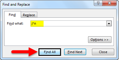
We will get the result as text ‘j*n’(john) is in the cell no. ‘A2’ because we have only one text which starts with ‘j’ and ends with ‘n’ with any number of characters between them.
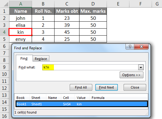
Use the question mark to find any single character.
Suppose we want to find text in the table that starts with the letter ‘k’ and ends with the letter ‘n’ with a single character. So, in the Find and Replace dialog box, we enter ‘k?n’ to find what box. Then click on Find All.
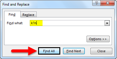
Here, we get the text ‘k?n’(kin) is in cell no. ‘A4’ because we have only one text which starts with ‘k’ and ends with ‘n’ with a single character between them.
- Click Options to further define your search if needed.
- We can find text or number by changing settings in the Within, Search and Look in the box according to our needs.
- To show the working of the above-mentioned options, we took the data as follows.
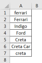
- To search case-sensitive data, select the Match case check box. It gives you output in the case you give input in the Find What box. For example, we have a table of some cars’ names. If you type ‘ferrari’ in the Find What box, then it will find only ‘ferrari’, not ‘Ferrari’.
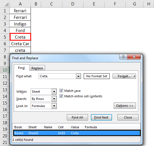
- To search for cells that contain just the characters you typed in the Find what box, select the Match entire cell contents checkbox. For example, we have a table of some cars’ names. Type ‘Creta’ in the Find What box.
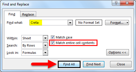
- It will then find cells containing exactly ‘Creta’, and cells containing ‘Cretaa’ or ‘Creta car’ will not be found.
- If you want to search for text or numbers with specific formatting, click Format, and then make your selections in the Find Format dialog box according to your need.
- Let us click the Font option and select the Bold, and click OK.
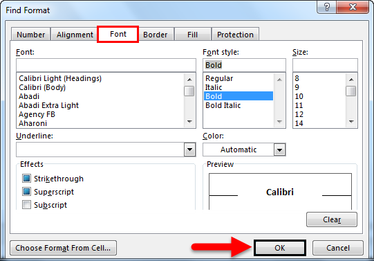
- Then, we click on Find All.
We get the value as ‘elisa’, which is in the ‘A3’ cell.
Method #2 – Using FIND Function in Excel
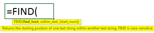
The FIND function in Excel gives the location of a substring within a string.
Syntax For FIND in Excel:
The first two parameters are required, and the last parameter is non-compulsory.
- Find_Value: The substring which you want to find.
- Within_String: The string in which you want to find the specific substring.
- Start_Position: It is a non-compulsory parameter and describes from which position we want to search substring. If you do not describe it, then start the search from the 1st position.
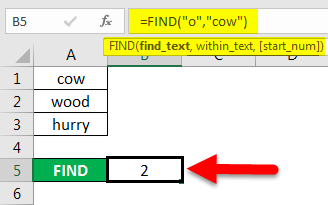
For example =FIND(“o”, “Cow”) gives 2 because “o” is the 2nd letter in the word “cow“.
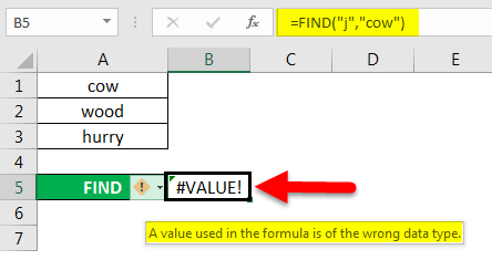
FIND(“j”, “Cow”) gives an error because there is no “j” in “Cow”.
- If the Find_Value parameter contains multiple characters, the FIND function gives the location of the first character.
E.g., the formula FIND(“ur”, “hurry”) gives 2 because “u” in the 2nd letter in the word “hurry”.

- If Within_String contains multiple occurrences of Find_Value, the first occurrence is returned. For example, FIND (“o”, “wood”)
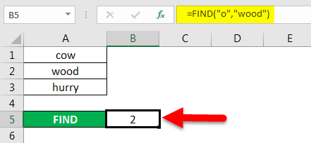
gives 2, which is the location of the first “o” character in the string “wood”.
The Excel FIND function gives the #VALUE! error if:
- If Find_Value does not exist in Within_String.
- If Start_Position contains multiple characters as compared to Within_String.
- If Start_Position either has a zero or negative number.
Method #3 – Using SEARCH Function in Excel
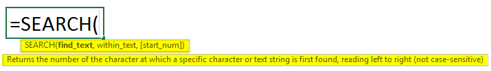
The SEARCH function in Excel is simultaneous to FIND because it also gives the location of a substring in a string.
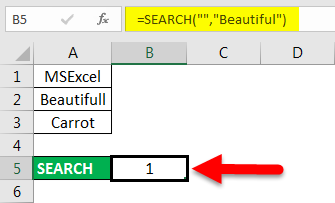
- If Find_Value is the blank string “, the Excel FIND formula gives the string’s first character.
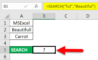
Example =SEARCH (“ful“, “Beautiful) gives 7 because the substring “ful” begins at the 7th position of the substring “beautiful”.
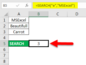
=SEARCH (“e”, “MSExcel”) gives 3 because “e” is the 3rd character in the word “MSExcel” and ignoring the case.
- Excel’s SEARCH function gives the #VALUE! error if:
- If the value of the Find_Value parameter is not found.
- If the Start_Position parameter is superior to the length of Within_String.
- If the Start_Position either equal to or less than 0.
Things to Remember About Find in Excel
- Asterisk defines a string of characters, and the question mark defines a single character. You can also find asterisks, question marks, and tilde characters (~) in worksheet data by preceding them with a tilde character inside the Find what option.
For example, to find data that contain “*”, you would type ~* as your search criteria.
- If you want to find cells that match a specific format, you can delete any criteria in the Find what box and select a specific cell format as an example. Click the arrow next to Format, click Choose Format From Cell, and click the cell with the formatting you want to search for.
- MSExcel saves the formatting options you define; you should clear the formatting options from the last search by clicking on an arrow next to Format and then Clear Find Format.
- The FIND function is case sensitive and does not allow while using wildcard characters.
- The SEARCH function is case-insensitive and allows while using wildcard characters.
Recommended Articles
This is a guide to Find in Excel. Here we discuss how to use the Find feature, Formula for FIND, and SEARCH in Excel, along with practical examples and a downloadable excel template. You can also go through our other suggested articles –
- FIND Function in Excel
- Excel SEARCH Function
- Find and Replace in Excel
- Search For Text in Excel
The FIND function is a built-in Worksheet Function (WS) in Microsoft Excel, which you can use to locate a sub-string or a specific character’s position within a text string. It is categorized as a TEXT function in Excel.
If the FIND function fails to find the text, it will return a #VALUE error. Note that the Excel FIND function will perform a case-sensitive search.
Excel FIND function is commonly used by financial analysts for locating specific data or text occurrences in a cell.

Syntax of Excel FIND function
=FIND(find_text, within_text, [start_num])
Arguments:
'find_text' – The text/sub-string you want to locate.'within_text' – This argument is the string within which you wish to perform the search. You can supply a cell reference or type in the string into the formula.'start_num' – This is an optional argument wherein you specify the character from which your search must begin. If you omit this argument, the function will assume this parameter as 1, i.e., the search will begin from the 1st character of the 'within_text' string.
Things to Remember
- The FIND function in Excel is case-sensitive and does not allow the usage of wildcard characters. For locating case-insensitive matches, take a look at the SEARCH function.
- The FIND function will search the
'find_text'argument in'within_text'and return the first character’s position. - You may search for either a substring or a character with the
'find_text'argument. You may use cell references or text characters for both'find_text'and'within_text'The FIND function will return ‘1’ when the'find_text'argument is an empty string «». - The FIND function returns #VALUE! error when:
- The FIND function cannot locate
'find_text'in'within_text'or - The
'start_num'argument is negative, 0, or greater than the length of'within_text'
- The FIND function cannot locate
Examples of FIND function in Excel
Example 1 – Finding a word’s position in a text string

In this example, when you search for «Dallas» and reference the cell A2, which has the text string «Dallas, USA» the function will return ‘1’. Here, 1 represents the position of the searched word’s starting point.
On account of the FIND function’s case-sensitivity, entering «dallas» as an argument will return #VALUE! error.
Example 2 – Search for a word in a text string

The 'start_num' argument lets you decide the starting position for performing the search in the text string. You will see that in the above example, the FIND function returns ‘1’ when we put 1 as the 'start_num'. Essentially, it searches for the text «Dallas» in «Dallas, USA».
When we change 'start_num' to ‘2’, it returns an error because it then searches for «Dallas» in «allas, USA».
Note that skipping the 'start_num' argument will result in the FIND function assuming ‘1’ as the starting position.
Example 3 – When the searched text occurs multiple times in a text string

Since the FIND function refers to the 'start_num' argument to see if you would like to define a starting position, it returns ‘1’ when you input 'start_num' as 1. This is because it finds «Dallas» at position ‘1’ in «Dallas, Dallas, USA».
When you input 'start_num' as 2, though, you will see that it returns ‘9’. What is happening here is that the FIND function tries to look for the word «Dallas» in «allas, Dallas, USA» since you are asking the function to start searching from the second position. Here, 9 is the starting position of the 2nd «Dallas» in «Dallas, Dallas, USA».
Example 4 – Look for a specific character’s Nth occurrence in a string.

Let’s now assume that you would like to know the position of the second «,» in the list that has the format «City, Country, Continent».
For this, we will need to nest two FIND functions one within another. The second FIND function will go in the first FIND function as a third argument ('start_num'), like so:
=FIND(",",A2,FIND(",",A2)+1)
With the third argument, you are instructing the first FIND function to start searching for «,» exactly after the first occurrence of a «,» in the string.
Pro tip: You can use the CHAR and SUBSTITUTE functions to do this more simply, with the following formula:
=FIND(CHAR(1), SUBSTITUTE(A5,",",CHAR(1),2)
Example 5 – Retrieving the first part of a text string separated by «,» (comma)

Let’s assume you want the list of just the name of cities, without the name of the country, i.e., the characters right before «,»).
To accomplish this, we will use the LEFT function and the FIND function together. The FIND function will give us the position of «,» and the LEFT function will allow us to retrieve the name of the cities.
In our example, the FIND function will return 10 when executed on «Amsterdam, Netherlands». From this, we will subtract 1 since we don’t want to include the «,» in our output.
Next, we embed a FIND function into the LEFT function and use FIND(",", A2,1)-1 as the second argument, like so:
=LEFT(A2,FIND(",",A2,1)-1)
Example 6 – Retrieving the second part of a text string separated by «,» (comma)

Let’s take example 5, and try to retrieve the second part of the string.
To accomplish this, we will use the MID function and the FIND function together. The FIND function will give us the position of «,» and the MID function will allow us to fetch the specific string portion that we need.
In our example, the FIND function will return 10 when executed on «Amsterdam, Netherlands». From this, we will add 1 since we don’t want to include the «,» in our output.
Next, we use a MID function and pass the FIND function to it FIND(",", A2,1)+1 as the second argument, like so:
=MID(A2,FIND(",",A2,1)+1,100)
FIND function vs. SEARCH function in Excel
Both Find and Search functions have a similar syntax and application. However, there are 2 differences between these functions. Let’s dive into what these differences are:
1. Acceptance of wildcard characters
Unlike with the FIND function, you may use wildcard characters in the SEARCH function’s 'find_text' argument.
To match one character – we will use a question mark ‘?’, and to match a series of characters – we will use an asterisk mark ‘*’.
Let’s work this out with an example:

We will use the syntax:
=SEARCH(",*EUROPE",A2)
Notice how the Excel SEARCH function returns the first character’s position if you input both «,» and the «continent name» regardless of how many characters exist between the text string referred to in the 'within_text'argument.
Pro tip: For finding a ‘?’ or ‘*’, just add a tilde (~) in front of the question mark or the asterisk.
2. FIND is case-sensitive, while SEARCH is case-insensitive
As I mentioned previously, case-sensitivity is another differentiating factor between the two functions.

In our example, when using the FIND function to search for ‘A’ it returns the position of the capital A in ‘USA’. However, searching for ‘A’ with the SEARCH function returns the position of the ‘a’ in ‘Dallas’ because it is case-insensitive.
Handling #VALUE! errors in the FIND function
To deal with #VALUE! errors, we can use the IFERROR function.
Let’s revisit our first example where we first encountered a #VALUE! error with FIND function on account of the FIND function’s case-sensitivity.

Here is the syntax we will use to fix this:
=IFERROR(FIND("dallas",A3,1), "Not Found!")
Using this syntax, we will «trap» the error and replace it with a standard string in the second argument of the IFERROR function, which in our case is «Not Found!». So, until the FIND function is able to return a matched string, the function will keep returning «Not Found».
The SEARCH function in Excel is categorized under text or string functions, but the output returned by this function is an integer. The SEARCH function gives us the position of a substring in a given string when we provide a parameter of the position to search from. Thus, this formula takes three arguments: substring, the string itself, and position to start the search.
For example, suppose we want to search the “Thank” substring in the provided text or string “Thank you.” Here, we need to find the “Thank” word using the SEARCH function, which will return the word “Thank” location.
=SEARCH(“Thank,” B8). The output will be 1.
The SEARCH function is a text function used to find the location of a substring in a string/text.
The SEARCH function can be used as a worksheet function. It is not case-sensitive.
Table of contents
- Excel SEARCH Function
- SEARCH Formula in Excel
- Explanation
- How to Use the Search Function in excel? (with Examples)
- Example #1
- Example #2
- Example #3
- Example #4
- Things to Remember
- Search Function in Excel Video
- Recommended Articles
SEARCH Formula in Excel
Below is the SEARCH formula in Excel.

Explanation
Excel SEARCH function has three-parameter two (find_text, within_text) are compulsory parameters and one (start_num) is optional.
Compulsory Parameter:
- find_text: find_text refers to the substring/character you want to search within a string or the text you want to find out.
- within_text:. Where your substring is located or where you perform the find_text.
Optional Parameter:
- [start_num]:: from where you want to start the SEARCH within the text in excelExcel provides the functionality that helps you to search for text in the file. You can use Find and Search function to search for a specific text cell value and arrive at the result.read more. If omitted, SEARCH considers it as 1 and star search from the first character.
How to Use the Search Function in excel? (with Examples)
The SEARCH function is very simple and easy to use. Let us understand the working of the SEARCH function in some examples.
You can download this Search Function Excel Template here – Search Function Excel Template
Example #1
Let us search the “Good” substring in the given text or string. Here, we have found the “Good” word using the SEARCH function, which will return the word “Good” location in the “Good morning.”
=SEARCH(“Good,” B6) and output will be 1.
Suppose two matches are found for “Good,” then SEARCH in Excel will give you the first match value. However, if you want the other good location, then you use the =SEARCH(“Good,” B7, 2) [start_num] as 2 then it will give you the place of the second match value, and the output will be 6.

Example #2
In this example, we will filter out the first and last names from the full names using the SEARCH in excelSearch function gives the position of a substring in a given string when we give a parameter of the position to search from. As a result, this formula requires three arguments. The first is the substring, the second is the string itself, and the last is the position to start the search.read more.
For first name=LEFT(B12,SEARCH(” “,B12)-1)

For last name=RIGHT(B12,LEN(B12)-SEARCH(” “,B12))

Example #3
Suppose there is a set of IDs. First, you have to find the _ location within IDs, then use Excel SEARCH to find the “_” location within IDs.
=SEARCH(“_,” B27), and output will be 6.

Example #4
Let us understand the working of SEARCH in excel with wildcards charactersIn Excel, wildcards are the three special characters asterisk, question mark, and tilde. Asterisk denotes multiple characters, a question mark denotes a single character, and a tilde denotes the identification of a wild card character.read more.

Consider the table and search for the next 0 within the text A1-001-ID.
And start position will be 1, then =SEARCH(“?” &I8, J8, K8) output will be 3 because “?” neglects the one character before the 0, and output will be 3.
For the second row within a given table, the search result for A within B1-001-AY.
It will be 8, but if we use “*” in search, it will give you the 1 as location output because it will neglect all characters before “A,” and output will be 1 for it =SEARCH(“*” &I9, J9).
Similarly, for “J” 8 =SEARCH(I10,J10,K10) and 7 for =SEARCH(“?”&I10,J10,K10).
Similarly, for fourth row, the output will be 8 for =SEARCH(I11,J11,K11) and 1 for =SEARCH(“*” &I11,J11,K11)
Things to Remember
- It is not case-sensitive.
- It considers tanuj and TANUJ as the same value, which means it does not distinguish between lower and upper case.
- It is also allowed wildcard characters, i.e., “?”, “*,” and “~” tilde.
- “?” is used to find a single character.
- “*” is used for match sequences.
- If we want to search the “*” or”? “, we need to insert the “~” before the character.
- It returns the #VALUE! Error if there is no matching string is found in the within_text.
Suppose in the below example. We are searching for a substring “a” within the “Name” column. If found, it will return the location of a within name else. In addition, it will give a #VALUE error#VALUE! Error in Excel represents that the reference cell the user has either entered an incorrect formula or used a wrong data type (mostly numerical data). Sometimes, it is difficult to identify the kind of mistake behind this error.read more, as shown below.

Search Function in Excel Video
Recommended Articles
This article is a guide to the SEARCH Function in Excel. Here, we discuss the SEARCH formula and how to use the SEARCH function, along with Excel examples and downloadable Excel templates. You may also look at these useful functions in Excel: –
- Search Box in ExcelA search box in Excel finds the needed data by typing into it, then filters the data and displays only that much info. When working with large datasheets, this simple tool may save a lot of time.read more
- Excel Substring FunctionThe substring function in Excel is a built-in integrated function that is categorized under the TEXT function and is used to extract a string from a combination of string.read more
- Filters in Excel
- True Function in Excel

In this article, we will learn How to use the FIND function in Excel.
Find any text in Excel
In Excel, you need to find the position of a text. Either you can count manually watching closely each cell value. Excel doesn’t want you to do that and neither do we. For example finding the position of space character to divide values wherever space exists like separating first name and last name from the full name. So let’s see the FIND function syntax and an example to illustrate its use.
In the cell Jimmy Kimmel, Space character comes right after the y and before K. 6th is the occurrence of Space char in word starting from J.
FIND Function in Excel
FIND function just needs two arguments (third optional). Given a partial text or single character to find within a text value is done using the FIND function.
FIND function Syntax:
=FIND(find_text, within_text, [start_num])
Find_text : The character or set of characters you want to find in string.
Within_text : The text or cell reference in which you want to find the text
[start_num] : optional. The starting point of search.
Example :
All of these might be confusing to understand. Let’s understand how to use the function using an example. Here Just to explain FIND function better, I have prepared this data.
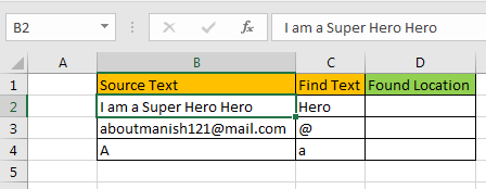
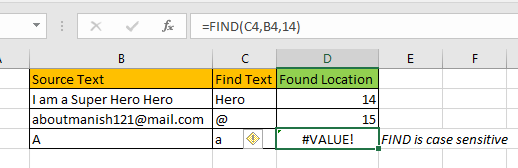
In Cell D2 to D4, I want to find the location of “Hero” in cell B2, “@” in cell B3 and “a” in B4, respectively.
I write this FIND formula in Cell D2 and drag it down to cell D4.
Use the Formula in D4 cell
And now i have the location of the given text:
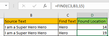
Find the Second, Third and Nth Occurrence of Given Characters in the Strings.
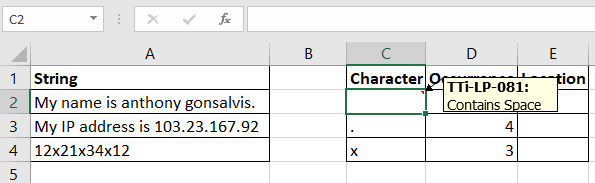
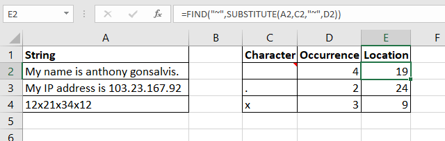
Here we have some strings in range A2:A4. In cell C2, C3, and C4 we have mentioned the characters that we want to search in the strings. In D2, D3, and D4 we have mentioned the occurrence of the character. In the adjacent cell I want to get the position of these occurrences of the characters.
Write this formula in the cell E2 and drag down.
This returns the exact positions (19) of the mentioned occurrence (4) of the space character in the string.
How does it work?
The technique is quite simple. As we know the SUBSTITUTE function of Excel replaces the given occurrence of a text in string with the given text. We use this property.
So the formula works from inside.
SUBSTITUTE(A2,C2,»~»,D2): This part resolves to SUBSTITUTE(«My name is anthony gonsalvis.«
,» «,»~»,4). Which ultimately gives us the string «My name is anthony~gonsalvis.«
P.S. : the fourth occurrence of space is replaced with «~». I replaced space with «~» because I am sure that this character will not appear in the string by default. You can use any character that you are sure will not appear in the string. You can use the CHAR function to insert symbols.
Search substring in Excel
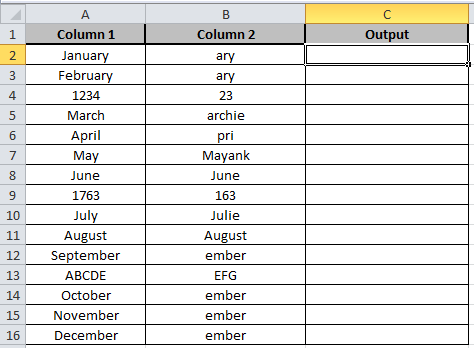
Here we have two columns. Substring in Column B and Given string in Column A.
Write the formula in the C2 cell.
Formula:
Explanation:
Find function takes the substring from the B2 cell of Column B and it then matches it with the given string in the A2 cell of Column A.
ISNUMBER checks if the string matches, it returns True else it returns False.
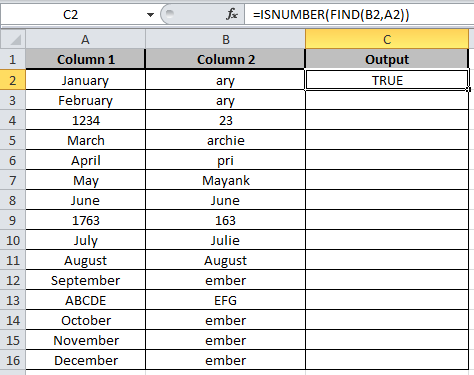
Copy the formula in other cells, select the cells taking the first cell where the formula is already applied, use shortcut key Ctrl + D.
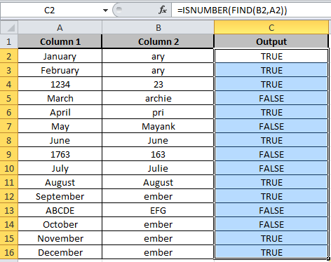
As you can see the output in column C shows True and False representing whether substring is there or not.
Here are all the observational notes using the FIND function in Excel
Notes :
FIND returns the first found location by default.
If you want a second found location of text then provide start_num and it should be greater than first location of the text.
If the given text is not found, FIND formula will return #VALUE error.
FIND is case sensitive. If you need an case insentive function, use the SEARCH function.

FIND does not support wildcard characters. Use the SEARCH function if you need to use wildcards to find text in a string.
Hope this article about How to use the FIND function in Excel is explanatory. Find more articles on searching partial text and related Excel formulas here. If you liked our blogs, share it with your friends on Facebook. And also you can follow us on Twitter and Facebook. We would love to hear from you, do let us know how we can improve, complement or innovate our work and make it better for you. Write to us at info@exceltip.com.
Related Articles :
How to use the SEARCH FUNCTION : It works same as the FIND function with only one difference of finding case insensitive ( like a or A are considered the same) in Excel.
Searching a String for a Specific Substring in Excel : Find cells if cell contains given word in Excel using the FIND or SEARCH function.
Highlight cells that contain specific text : Highlight cells if cell contains given word in Excel using the formula under Conditional formatting
How to Check if a string contains one of many texts in Excel : lookup cells if cell contains from given multiple words in Excel using the FIND or SEARCH function.
Count Cells that contain specific text : Count number of cells if cell contains given text using one formula in Excel.
How to lookup cells having certain text and returns the Certain Text in Excel : find cells if cell contains certain text and returns required results using the IF function in Excel.
Popular Articles :
How to use the IF Function in Excel : The IF statement in Excel checks the condition and returns a specific value if the condition is TRUE or returns another specific value if FALSE.
How to use the VLOOKUP Function in Excel : This is one of the most used and popular functions of excel that is used to lookup value from different ranges and sheets.
How to use the SUMIF Function in Excel : This is another dashboard essential function. This helps you sum up values on specific conditions.
How to use the COUNTIF Function in Excel : Count values with conditions using this amazing function. You don’t need to filter your data to count specific values. Countif function is essential to prepare your dashboard.
Purpose
Get location substring in a string
Return value
A number representing the location of substring
Usage notes
The FIND function returns the position (as a number) of one text string inside another. If there is more than one occurrence of the search string, FIND returns the position of the first occurrence. When the text is not found, FIND returns a #VALUE error. Also note, when find_text is empty, FIND returns 1. FIND does not support wildcards, and is always case-sensitive. Use the SEARCH function to find the position of text without case-sensitivity and with wildcard support.
Basic Example
The FIND function is designed to look inside a text string for a specific substring. When FIND locates the substring, it returns a position of the substring in the text as a number. If the substring is not found, FIND returns a #VALUE error. For example:
=FIND("p","apple") // returns 2
=FIND("z","apple") // returns #VALUE!
Note that text values entered directly into FIND must be enclosed in double-quotes («»).
Case-sensitive
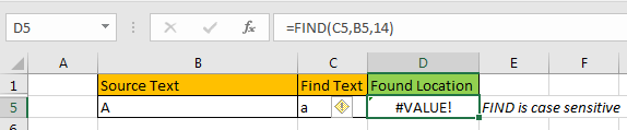
The FIND function always case-sensitive:
=FIND("a","Apple") // returns #VALUE!
=FIND("A","Apple") // returns 1
TRUE or FALSE result
To force a TRUE or FALSE result, nest the FIND function inside the ISNUMBER function. ISNUMBER returns TRUE for numeric values and FALSE for anything else. If FIND locates the substring, it returns the position as a number, and ISNUMBER returns TRUE:
=ISNUMBER(FIND("p","apple")) // returns TRUE
=ISNUMBER(FIND("z","apple")) // returns FALSE
If FIND doesn’t locate the substring, it returns an error, and ISNUMBER returns FALSE.
Start number
The FIND function has an optional argument called start_num, that controls where FIND should begin looking for a substring. To find the first match of «the» in any combination of upper or lowercase, you can omit start_num, which defaults to 1:
=FIND("x","20 x 30 x 50") // returns 4To start searching at character 5, enter 4 for start_num:
=FIND("x","20 x 30 x 50",5) // returns 9
Wildcards
The FIND function does not support wildcards. See the SEARCH function.
If cell contains
To return a custom result with the SEARCH function, use the IF function like this:
=IF(ISNUMBER(FIND(substring,A1)), "Yes", "No")
Instead of returning TRUE or FALSE, the formula above will return «Yes» if substring is found and «No» if not.
Notes
- The FIND function returns the location of the first find_text in within_text.
- The location is returned as the number of characters from the start.
- Start_num is optional and defaults to 1.
- FIND returns 1 when find_text is empty.
- FIND returns #VALUE if find_text is not found.
- FIND is case-sensitive but does not support wildcards.
- Use the SEARCH function to find a substring with wildcards.