Find duplicates in one column in excel - Word и Excel - помощь в работе с программами

Find and remove duplicates

Excel for Microsoft 365 Excel 2021 Excel 2019 Excel 2016 Excel 2013 Excel 2010 Excel 2007 Excel Starter 2010 More…Less

Sometimes duplicate data is useful, sometimes it just makes it harder to understand your data. Use conditional formatting to find and highlight duplicate data. That way you can review the duplicates and decide if you want to remove them.

Select the cells you want to check for duplicates.

Note: Excel can’t highlight duplicates in the Values area of a PivotTable report.
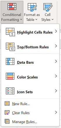
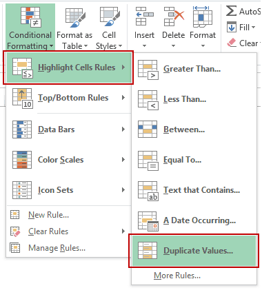
Click Home > Conditional Formatting > Highlight Cells Rules > Duplicate Values.
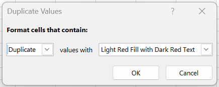
In the box next to values with, pick the formatting you want to apply to the duplicate values, and then click OK.

Remove duplicate values

When you use the Remove Duplicates feature, the duplicate data will be permanently deleted. Before you delete the duplicates, it’s a good idea to copy the original data to another worksheet so you don’t accidentally lose any information.

Select the range of cells that has duplicate values you want to remove.
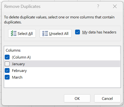
Click Data > Remove Duplicates, and then Under Columns, check or uncheck the columns where you want to remove the duplicates.

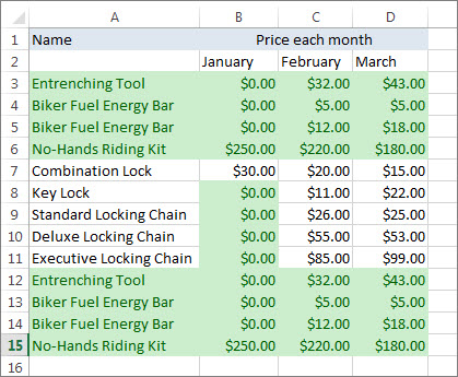
For example, in this worksheet, the January column has price information I want to keep.

So, I unchecked January in the Remove Duplicates box.
Click OK.

Note: The counts of duplicate and unique values given after removal may include empty cells, spaces, etc.

Need more help?

Источник

The searching of duplicates in Excel – is one of the most common tasks for any of office employee. For its solution, there are a few different methods. But – how quickly to find duplicates in Excel and to highlight them with color? For the answer on this frequently asked question let us consider a concrete example.

How to find duplicate values in Excel?

For example we are engaging by check orders, which coming into the firm through Fax and e-mail. There can be such situation that the same order was by the two channels of incoming information. If you register twice the same order, there can be certain problems for the firm. Below we are considering to the decision by means of the conditional formatting.

For avoiding of the duplicate orders, you can use to the conditional formatting, which helps you quickly to find the duplicate values in Excel column.

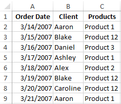
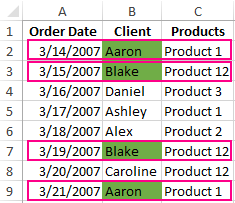
The example of the day orders for goods:

For verification whether the day orders are possible duplicates, we will analyze in the names of customers – there is the column B:

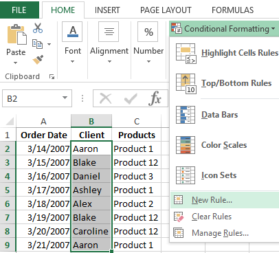
To highlight the range B2:B9 and then to select the instrument: «HOME» — «Styles» — «Conditional Formatting» — «New Rule».

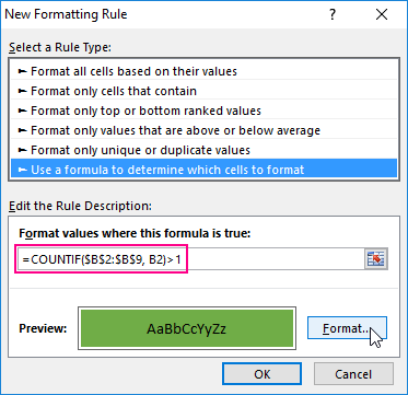
To choose «Use a formula to determine which cells to format».

To find the duplicate values in Excel column, you need to enter the formula in the input field:

After that you need to press the button «Format» and select to the desired cell shading to highlight duplicates in color — for example, green one. And click OK on all windows are opened.

Result.

Download an example of finding the Identifying Duplicate values in a column.

As can be seen in the picture with the conditional formatting we were able easily and quickly to implement the duplicate finder in function Excel and to detect to the duplicate data cells for the table of the day orders.

The example of COUNTIF function and highlighting of the duplicate values

The principle of the action formula for finding of the duplicates by the conditional formatting is simple. The formula contains the function =COUNTIF(). This function can also be used when searching for the identical values in the range of cells. The first argument in the function to the viewable data range is specified. In the second argument we specify what we are looking for. The first argument has an absolute reference, as it should be the same one. And the second argument conversely — should be changed on the address of the each cell in the viewing range, because it has a relative link one.

The fastest and the simplest ways: to find to the duplicates in the cells.

After the function we can see the comparison operator of the number of the found values in the range with the number 1. That is, if we see more, than one value means that the formula returns the value of TRUE and for the current cell is applied to the conditional formatting.

Источник

When you are working on a large number of data then you will encounter a few duplicate entries.

Sometimes these duplicate values are very useful but many times you want to remove the duplicate data. If you have 1000 data then it becomes quite difficult to find and remove the duplicate data.

Here we have provided the step-by-step process on how to find duplicates in excel.

Take a look and follow the process.

There are many ways to find duplicate items and values in excel. You might be thinking as to why should I apply any formula or method to find duplicate values as it is easy.

But it’s not about few data, you can apply a formula or method when you have lots of data.

The method or formula to find and remove the duplicate items make the process easier and saves your time. Here you can check three different processes.

1. Find Duplicates in Excel using Conditional Formatting

To find duplicate values in Excel, you can use conditional formatting excel formula, Vlookup, and Countif formula. After finding out the duplicate values, you can remove them if you want by using different methods that are described below.

Remove duplicate values

Select all the duplicate cells or highlighted cells
Delete the values by pressing the Delete button.
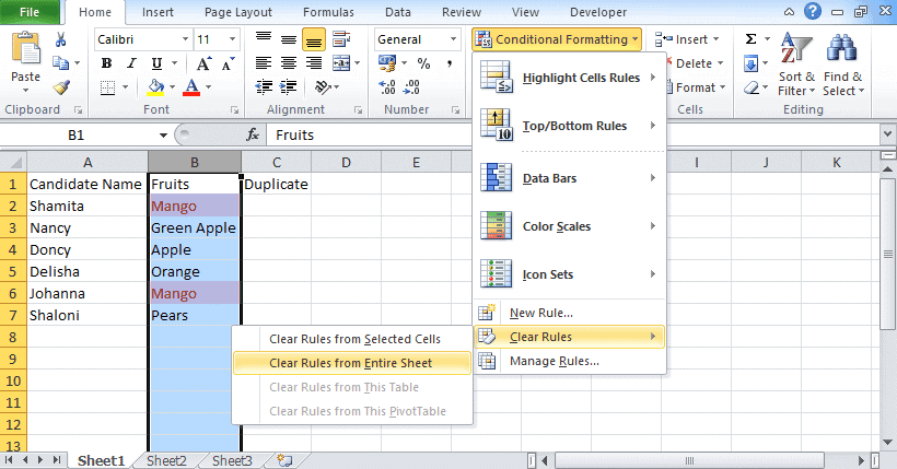
After deleting the values, go to the conditional formatting.
Choose Clear rules.
And then choose clear rules from an entire sheet.

Another way to remove the duplicate value

This method will delete all the duplicate data permanently. If you want the duplicate data again, then copy the data on another worksheet.

Select the cells on which you want to find and remove the duplicate values.
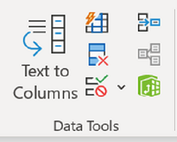
Go to the ribbon and find the data option.
In the data tab, you will find the remove duplicates option.
Now check or uncheck the column on which you want to apply this constraint.
Then click OK.

2. Find Duplicates in One Column using COUNTIF

Another way to detect duplicates is via the COUNTIF function. If you want to apply the COUNTIF function then check here how to find duplicates in Excel using the Excel COUNT function.

If you have the list of items from where you want to find duplicates, then you need to apply the COUNTIF formula to it.
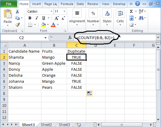
The syntax for COUNTIF: “=COUNTIF(B:B, B2)>1”.
In column A, you have the Buyer’s name and in column B, you have the fruits name that he or she likes. Now you want to find the duplicate items.
Put this COUNTIF formula in column C.
For all duplicate fields, it shows TRUE whereas, for non-duplicate fields, it shows FALSE.
Now by following the above step-by-step process, you can delete all the duplicate items that you do not need.

Find Duplicates in Two Columns in Excel

Above we have seen how to find duplicate values in one column, now we will see here how to find duplicates in two columns in excel.

In this example, we have taken a table where the candidate name is in column A and Fruits is in column B. Now we want to find duplicate values having the same name and fruits.

The formula to find duplicate values in two columns is

=If (Countifs($A$2:$A$8, $A2, $B$2:$B$8, $B2)>1, "Duplicate Values"," ")

How to Count Duplicates in Excel

If you want to know the total number of duplicate values then you need to use the Count function. For counting duplicate values you need to use the countif formula.

=Countif($A$2:$A$8, $A2)

3. Filter Duplicates in Excel

Another method to find duplicates in excel is to filter data to get duplicate values.

Remove Duplicates Online

To remove duplicates, you need to follow the below-mentioned process

Select the table by dragging the mouse.
Right-click on the table.
Delete the row by choosing the Delete Row option.

Highlight Duplicates in Excel

In order to highlight the duplicate values, you can either use a conditional formula to find duplicates in excel or follows the below-mentioned process.

Select the duplicate values.
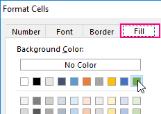
Go to the Fill color option and select the color.

This will highlight the duplicate values in excel.

Apart from these, there are other processes available by which you can find the duplicate items available in your data set. After finding out the duplicate values, you can remove them easily. Stay connected with our website to know other Excel features.

Related Queries

Here we have listed a few queries that are asked by Excel learners. If you are also facing this kind of problem then you can check it here.

Q1. How to delete duplicate e-mail addresses if you have 10,000 emails in your data set?

Ans. If you have all email addresses in a single column then select the column and go to the “Data” ribbon. You will find the ‘Remove Duplicates’ tab in data tools.

Click on Remove Duplicates and you will find another dialog box where you need to make a selection. Press Ok and you receive the unique email addresses.

Q2. How to find the repeated teacher’s name in Column A? The data is

B1= Maths/English Jasmine, Eon
B2= Physics Johana
B3= History Poole
B4= English/Physics Sam, Jasmine
B5= Chemistry Romeo

Ans. To solve this problem, create three separate columns. In the first column, mention the class name. In the second column, put the teacher’s name, and in the third mention another teacher’s name. Now in the fourth column, put the formula =COUNTIF(B:B,B1)>1

Using this formula, you will find “TRUE” if the value is duplicate.

Q3. How to sort data before applying a filter?

Ans. To sort data you need to choose the Sort tab in excel. Sorting a data set is quite an easy process. Follow the process mentioned below and sort your data completely.

Select the data set.
Go to the Data ribbon.
In the Sort & Filter section, you will find the Sort icon. Click on the icon and sort your data.

Q4. How to compare two columns in excel?

This question was mainly asked by the interviewer at the time of the interview. There are many ways to compare the two columns:

=A2=B2 This is the simple formula used to compare two columns.
Conditional Formatting: In this, you need to follow the above process, you can check the conditional formatting excel link to get detailed information.
Vlookup: You can also use the Vlookup formula to compare two columns using Vlookup for research, ISNA for performance, and If to customize the result.
Excel If Statement: This is a quite useful function in excel and it can be used in many ways. To get the detailed information Click Here.

Q5. How to filter data in excel?

Filtering in Excel is an easy process. In the sort & filter section, you will find the Filter icon. Click on the icon and filter your data.

In this tutorial, we have covered all the excel topics that are best for beginners and experts. We always try to solve all the problems that people face while working on excel. If you have any other query or want to ask something then you can mention in the comment box below. One of our team members will be back with the answer.

You may also like the following Excel tutorials:

How to Remove Formulas in Excel (and keep the data)
How to Fill Blank Cells with Value above in Excel
How to Generate Random Numbers in Excel (Without Duplicates)
How to Find Merged Cells in Excel
Highlight Cell If Value Exists in Another Column in Excel
Using Conditional Formatting with OR Criteria in Excel
How to Remove Duplicate Rows based on one Column in Excel?
Get Unique Values from a Column in Excel
How to Count Unique Values in Excel (Formulas)
How to Use Greater Than or Equal to Operator in Excel Formula?

Источник

Watch Video – How to Find and Remove Duplicates in Excel

With a lot of data…comes a lot of duplicate data.

Duplicates in Excel can cause a lot of troubles. Whether you import data from a database, get it from a colleague, or collate it yourself, duplicates data can always creep in. And if the data you are working with is huge, then it becomes really difficult to find and remove these duplicates in Excel.

In this tutorial, I’ll show you how to find and remove duplicates in Excel.

FIND and HIGHLIGHT Duplicates in Excel.
- Find and Highlight Duplicates in a Single Column.
- Find and Highlight Duplicates in Multiple Columns.
- Find and Highlight Duplicate Rows.
REMOVE Duplicates in Excel.
- Remove Duplicates from a Single Column.
- Remove Duplicates from Multiple Columns.
- Remove Duplicate Rows.

Find and Highlight Duplicates in Excel

Duplicates in Excel can come in many forms. You can have it in a single column or multiple columns. There may also be a duplication of an entire row.

Finding and Highlight Duplicates in a Single Column in Excel

Conditional Formatting makes it simple to highlight duplicates in Excel.

Here is how to do it:

Select the data in which you want to highlight the duplicates.

Go to Home –> Conditional Formatting –> Highlight Cell Rules –> Duplicate Values.

In the Duplicate Values dialog box, select Duplicate in the drop down on the left, and specify the format in which you want to highlight the duplicate values. You can choose from the ready-made format options (in the drop down on the right), or specify your own format.

This will highlight all the values that have duplicates.

Quick Tip: Remember to check for leading or trailing spaces. For example, “John” and “John ” are considered different as the latter has an extra space character in it. A good idea would be to use the TRIM function to clean your data.

Finding and Highlight Duplicates in Multiple Columns in Excel

If you have data that spans multiple columns and you need to look for duplicates in it, the process is exactly the same as above.

Here is how to do it:

Select the data.
Go to Home –> Conditional Formatting –> Highlight Cell Rules –> Duplicate Values.
In the Duplicate Values dialog box, select Duplicate in the drop down on the left, and specify the format in which you want to highlight the duplicate values.
This will highlight all the cells that have duplicates value in the selected data set.

Finding and Highlighting Duplicate Rows in Excel

Finding duplicate data and finding duplicate rows of data are 2 different things. Have a look:

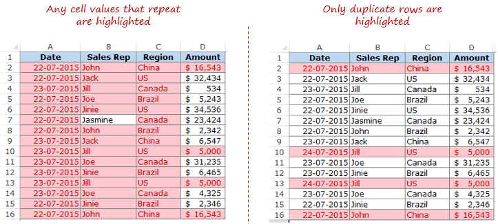Finding duplicate rows is a bit more complex than finding duplicate cells.

Here are the steps:

In an adjacent column, use the following formula:
=A2&B2&C2&D2
Drag this down for all the rows. This formula combines all the cell values as a single string. (You can also use the CONCATENATE function to combine text strings)

By doing this, we have created a single string for each row. If there are duplicate rows in this dataset, then these strings would be exactly the same for it.

Now that we have the combined strings for each row, we can use conditional formatting to highlight duplicate strings. A highlighted string implies that the row has a duplicate.

Here are the steps to highlight duplicate strings:

Select the range that has the combined strings (E2:E16 in this example).
Go to Home –> Conditional Formatting –> Highlight Cell Rules –> Duplicate Values.
In the Duplicate Values dialog box, make sure Duplicate is selected and then specify the color in which you want to highlight the duplicate values.

This would highlight the duplicate values in column E.

In the above approach, we have highlighted only the strings that we created.

But what if you want to highlight all the duplicate rows (instead of highlighting cells in one single column)?

Here are the steps to highlight duplicate rows:

In an adjacent column, use the following formula:
=A2&B2&C2&D2
Drag this down for all the rows. This formula combines all the cell values as a single string.

Select the data A2:D16.
With the data selected, go to Home –> Conditional Formatting –> New Rule.

In the ‘New Formatting Rule’ dialog box, click on ‘Use a formula to determine which cells to format’.
In the field below, use the following COUNTIF function:
=COUNTIF($E$2:$E$16,$E2)>1

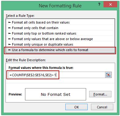
Select the format and click OK.

This formula would highlight all the rows that have a duplicate.

Remove Duplicates in Excel

In the above section, we learned how to find and highlight duplicates in excel. In this section, I will show you how to get rid of these duplicates.

Remove Duplicates from a Single Column in Excel

If you have the data in a single column and you want to remove all the duplicates, here are the steps:

Select the data.
Go to Data –> Data Tools –> Remove Duplicates.
In the Remove Duplicates dialog box:
- If your data has headers, make sure the ‘My data has headers’ option is checked.
- Make sure the column is selected (in this case there is only one column).

Click OK.

This would remove all the duplicate values from the column, and you would have only the unique values.

CAUTION: This alters your data set by removing duplicates. Make sure you have a back-up of the original data set. If you want to extract the unique values at some other location, copy this dataset to that location and then use the above-mentioned steps. Alternatively, you can also use Advanced Filter to extract unique values to some other location.

Remove Duplicates from Multiple Columns in Excel

Suppose you have the data as shown below:

In the above data, row #2 and #16 have the exact same data for Sales Rep, Region, and Amount, but different dates (same is the case with row #10 and #13). This could be an entry error where the same entry has been recorded twice with different dates.

To delete the duplicate row in this case:

Select the data.
Go to Data –> Data Tools –> Remove Duplicates.
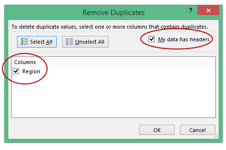
In the Remove Duplicates dialog box:
- If your data has headers, make sure the ‘My data has headers’ option is checked.
- Select all the columns except the Date column.

Click OK.

This would remove the 2 duplicate entries.

NOTE: This keeps the first occurrence and removes all the remaining duplicate occurrences.

Remove Duplicate Rows in Excel

To delete duplicate rows, here are the steps:

Select the entire data.
Go to Data –> Data Tools –> Remove Duplicates.
In the Remove Duplicates dialog box:
- If your data has headers, make sure the ‘My data has headers’ option is checked.
- Select all the columns.

Click OK.

Use the above-mentioned techniques to clean your data and get rid of duplicates.

You May Also Like the Following Excel Tutorials:

10 Ways to Clean Data in Excel Spreadsheets.
Remove Leading and Trailing Spaces in Excel.
24 Daily Excel Issues and their Quick Fixes.
How to Find Merged Cells in Excel.

Источник

In MS Excel, the duplicate values can be found and removed from a data set. Depending on your data and requirement, the most commonly used methods are the conditional formatting feature or the COUNTIF formula to find and highlight the duplicates for a specific number of occurences. The columns of the data set can be then filtered to view the duplicate values.

In this article, we will look at 5 different methods to check, identify, and delete duplicates in Excel.

How to Find Duplicates in Excel?
- 5 Methods to Check & Identify Duplicates in Excel
  - #1 – Conditional Formatting
  - #2 – Conditional Formatting (Specific Occurrence)
  - #3 – Change Rules (Formulas)
  - #4 – Remove Duplicates
  - #5 – COUNTIF Formula
- Frequently Asked Questions
- Recommended Articles

5 Methods to Check & Identify Duplicates in Excel

You can download this Find for Duplicates Excel Template here – Find for Duplicates Excel Template

#1 – Conditional Formatting

The conditional formattingConditional formatting is a technique in Excel that allows us to format cells in a worksheet based on certain conditions. It can be found in the styles section of the Home tab.read more feature is available in Excel 2007 and subsequent versions.

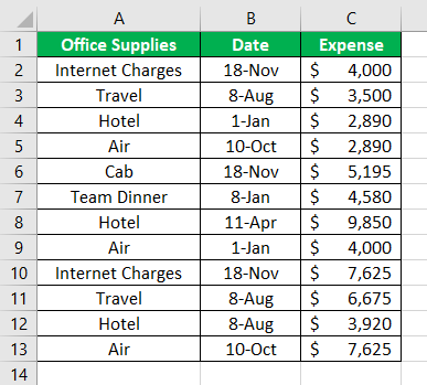
The following table consists of the expenses incurred on availing certain office facilities. The corresponding dates of purchasing such facility are also listed.

We want to identify the duplicates in excel with the help of conditional formatting.

The steps to find the duplicates in excel with the help of conditional formatting are listed as follows:

Select the data range (A1:C13) where duplicates are to be found.
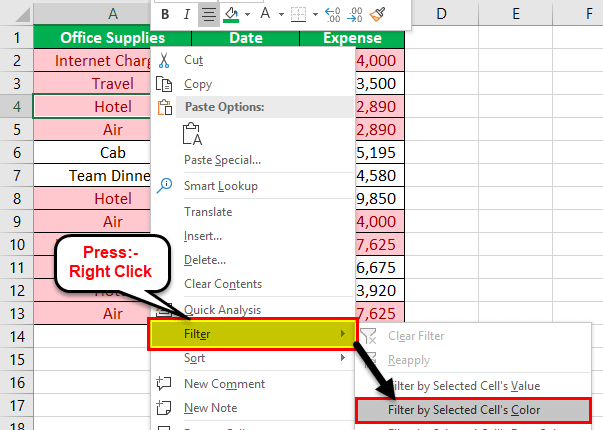
In the Home tab, select “conditional formatting” from the “styles” section. From the drop-down menu, select “highlight cell rules” and click on “duplicate values.”
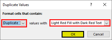
The pop-up window titled “duplicate values” appears. In the first box on the left side, select “duplicate.” In the “values with” drop-down, select the required color to highlight the duplicate cells. Click “Ok.”
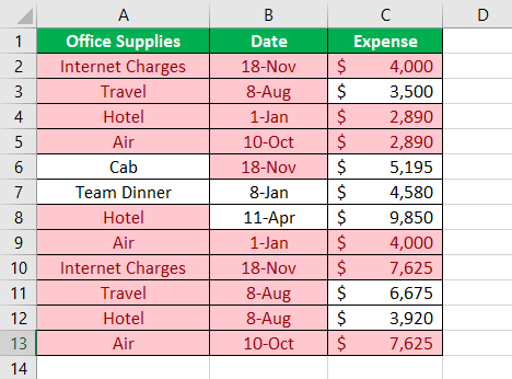
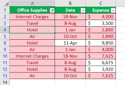
The duplicate cells are highlighted in the data table, as shown in the following image.
The columns can be filtered to identify the duplicate values. For this, right-click the required column and select “filter by selected cell’s color.” The data is filtered for duplicates.
The result after applying the filter to the first column (office supplies) is shown in the following image.

#2 – Conditional Formatting (Specific Occurrence)

Let us consider an example to identify the specific number of duplications. In the following table, we want to check and show the duplicate values with three occurrences.

The steps to find the duplicate values for specific number of occurrences are listed as follows:

Step 1: Select the range A2:C8 in the given data table.

Step 2: In the Home tab, select “conditional formatting” from the “styles” section. Click “new rule.”

Note: The “new rule” option helps highlight a specific count of duplicates using the COUNTIF formula.

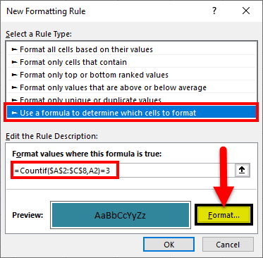
Step 3: The pop-up window titled “new formatting rule” appears. Enter the following details, as shown in the succeeding image.

Under “select a rule type,” select “use a formula to determine which cells to format.”
Under “edit the rule description,” enter the COUNTIFThe COUNTIF function in Excel counts the number of cells within a range based on pre-defined criteria. It is used to count cells that include dates, numbers, or text. For example, COUNTIF(A1:A10,”Trump”) will count the number of cells within the range A1:A10 that contain the text “Trump”
read more formula.

The COUNTIF formula “=COUNTIF(cell range of the data table, cell criteria)” finds and highlights the cells for the desired number of occurrences.

In this case, the COUNTIF formula highlights duplicate cells having triplicate count. This count can be changed to a greater number. The conditions can also be changed depending on the user’s requirement.

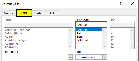
Step 4: Once the COUNTIF formula is entered, click “format.” The pop-up window titled “format cells” opens. Select the font style “regular.”

Step 5: In the “fill” tab, select blue color. The “fill” tab helps highlight the duplicate cellsHighlight Cells Rule, which is available under Conditional Formatting under the Home menu tab, can be used to highlight duplicate values in the selected dataset, whether it is a column or row of a table.read more.

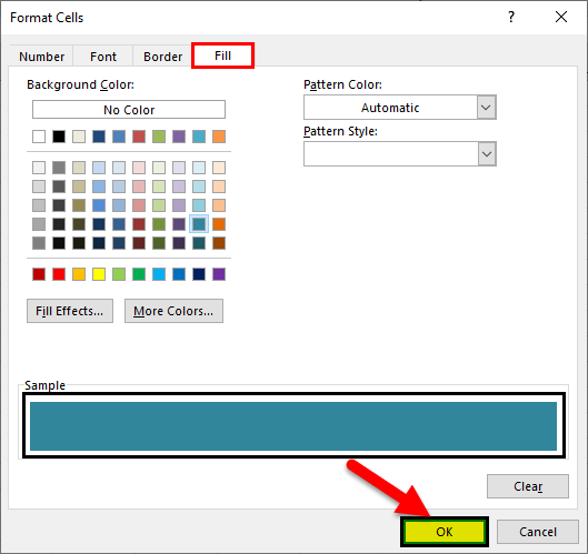
Step 6: Once the selections in “format cells” window are complete, click “Ok.” Click “Ok” again in the “new formatting rule” window.

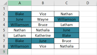
Step 7: The result is displayed in the following image. The duplicate cells with three occurrences are highlighted.

#3 – Change Rules (Formulas)

Working on the data of example #2, let us understand the procedure of changing the formula. For applying new formulas, the existing rules (formulas) of the data tableA data table in excel is a type of what-if analysis tool that allows you to compare variables and see how they impact the result and overall data. It can be found under the data tab in the what-if analysis section.read more have to be cleared.

The steps to clear the existing rules (shown in the succeeding image) are listed as follows:

Step 1: In the Home tab, select “conditional formatting” from the “styles” section.

Step 2: In “clear rules” option, select either of the following:

Clear rules from selected cells–This resets the rules for the selected range of the table. So, prior to clearing the rules, the data needs to be selected.
Clear rules from entire sheet–This clears the rules for the entire sheet.

The blue highlighted cells disappear and the original table is displayed.

#4 – Remove Duplicates

Let us check and delete duplicate values from a selected range. Prior to deletion, keeping a copy of the table is advisable because the duplicates will be permanently deleted.

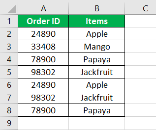
The following table displays a series of items with their corresponding IDs.

The steps to find and delete duplicate values are listed as follows:

Step 1: Select the range of the table whose duplicates are required to be deleted.

Step 2: In the Data tab, select “remove duplicates” from the “data tools” section.

Note: The “remove duplicates” option helps eliminate duplicates and retain unique cell values.

Step 3: The pop-up window titled “remove duplicates” appears, as shown in the succeeding image. By default, the following options are already selected:

The checkboxes for both the headers (“order ID” and “items”)
The “select all” box

Since the table consists of column headers, select the checkbox “my data has headers.” Click “Ok” to execute.

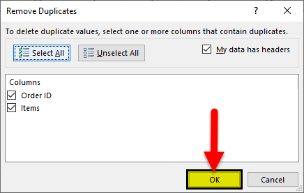
Note: To change the number of columns selected, click “unselect all.” Following this, the desired columns from which the duplicates are to be deleted can be selected.

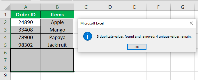
Step 4: The result is shown in the succeeding image. A prompt is displayed which states the following details:

The number of duplicate values removed from the table
The number of unique values that remain in the table after deletion

Click “Ok.” Hence, the duplicate values along with their corresponding rows are deleted.

#5 – COUNTIF Formula

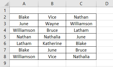
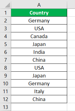
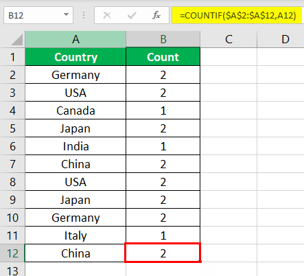
The following table displays the names of a few countries. We want to identify the duplicate values using the COUNTIF function.

The COUNTIF function requires the range (column containing duplicate entries) and the cell criteria. It returns the number of corresponding duplicates for every cell.

The steps to find the duplicate values in excel with the help of the COUNTIF function are listed as follows:

Step 1: Enter the formula shown in the succeeding image. Press the “Enter” key.

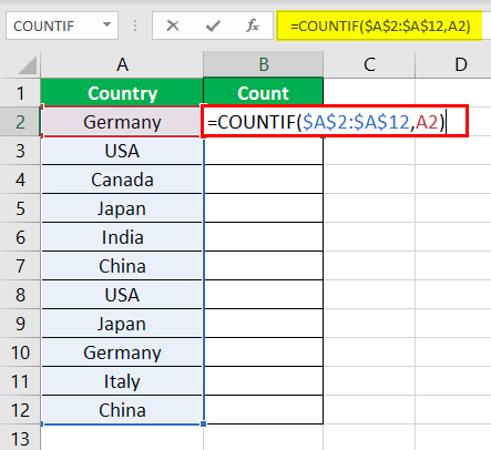
Note: The range must be fixed with the dollar ($) sign. Otherwise, the cell reference will change on dragging the formula.

Step 2: Drag the formula till the end of the table with the help of the fill handle. Alternatively, place the cursor on cell B2 and double-click the fill handle. The fill handle appears at the lower right corner of cell B2.

Step 3: The output of the formula is shown in the following image. It returns the count of duplicates for the entire data set.

Note: The filter can be applied to the column header to view the occurrences greater than one.

Frequently Asked Questions

1. What does it mean to find duplicates in Excel?

While consolidating different worksheets, several duplicates may be found in a data set. MS Excel helps to find and highlight such duplicates. It is also possible to filter a column for duplicate values.

An easy way to search for duplicates is by using the COUNTIF formula. This formula can count the total number of duplicates in a column. It can also count the number of individual instances of a particular duplicate entry. It accepts two arguments–the range and the criteria.

2. How to find duplicates in a column of Excel?

To check a column for duplicates, the formula is given as follows:

“=COUNTIF(A:A,A2)>1”

The formula checks for duplicates in column A. The topmost cell is A2. For every duplicate value, the formula returns “true.” For every unique value, the formula returns “false.”

Note: For an output other than “true” and “false,” the COUNTIF formula can be enclosed in the IF function.

3. What is the formula to find duplicates in Excel?

The generic formula to find the exact, case-sensitive duplicate values is stated as follows:
“IF(SUM((-EXACT(range,uppermost_cell)))<=1,””,”Duplicate”)”

The EXACT function compares the cell range with the target cell. The SUM function adds the number of instances. If the occurrence is greater than 1, the IF function returns “duplicate.”
Note 1: Since it is an array formula, it should be entered using “Ctrl+Shift+Enter.”

Note 2: If the same word appears twice in lowercase and once in uppercase, the formula will not count the uppercase word as duplicate.

Video Tutorial

What Is A Duplicate Value?

Duplicate values happen when the same value or set of values appear in your data.

For a given set of data you can define duplicates in many different ways.

In the above example, there is a simple set of data with 3 columns for the Make, Model and Year for a list of cars.

The first image highlights all the duplicates based only on the Make of the car.
The second image highlights all the duplicates based on the Make and Model of the car. This results in one less duplicate.
The second image highlights all the duplicates based on all columns in the table. This results in even less values being considered duplicates.

The results from duplicates based on a single column vs the entire table can be very different. You should always be aware which version you want and what Excel is doing.

Find And Remove Duplicate Values With The Remove Duplicates Command

Removing duplicate values in data is a very common task. It’s so common, there’s a dedicated command to do it in the ribbon.

Select a cell inside the data which you want to remove duplicates from and go to the Data tab and click on the Remove Duplicates command.

Excel will then select the entire set of data and open up the Remove Duplicates window.

You then need to tell Excel if the data contains column headers in the first row. If this is checked, then the first row of data will be excluded when finding and removing duplicate values.
You can then select which columns to use to determine duplicates. There are also handy Select All and Unselect All buttons above you can use if you’ve got a long list of columns in your data.

When you press OK, Excel will then remove all the duplicate values it finds and give you a summary count of how many values were removed and how many values remain.

This command will alter your data so it’s best to perform the command on a copy of your data to retain the original data intact.

Find And Remove Duplicate Values With Advanced Filters

There is also another way to get rid of any duplicate values in your data from the ribbon. This is possible from the advanced filters.

Select a cell inside the data and go to the Data tab and click on the Advanced filter command.

This will open up the Advanced Filter window.

You can choose to either to Filter the list in place or Copy to another location. Filtering the list in place will hide rows containing any duplicates while copying to another location will create a copy of the data.
Excel will guess the range of data, but you can adjust it in the List range. The Criteria range can be left blank and the Copy to field will need to be filled if the Copy to another location option was chosen.
Check the box for Unique records only.

Press OK and you will eliminate the duplicate values.

Advanced filters can be a handy option for getting rid of your duplicate values and creating a copy of your data at the same time. But advanced filters will only be able to perform this on the entire table.

Find And Remove Duplicate Values With A Pivot Table

Pivot tables are just for analyzing your data, right?

You can actually use them to remove duplicate data as well!

You won’t actually be removing duplicate values from your data with this method, you will be using a pivot table to display only the unique values from the data set.

First, create a pivot table based on your data. Select a cell inside your data or the entire range of data ➜ go to the Insert tab ➜ select PivotTable ➜ press OK in the Create PivotTable dialog box.

With the new blank pivot table add all fields into the Rows area of the pivot table.

You will then need to change the layout of the resulting pivot table so it’s in a tabular format. With the pivot table selected, go to the Design tab and select Report Layout. There are two options you will need to change here.

Select the Show in Tabular Form option.
Select the Repeat All Item Labels option.

You will also need to remove any subtotals from the pivot table. Go to the Design tab ➜ select Subtotals ➜ select Do Not Show Subtotals.

You now have a pivot table that mimics a tabular set of data!

Pivot tables only list unique values for items in the Rows area, so this pivot table will automatically remove any duplicates in your data.

Find And Remove Duplicate Values With Power Query

Power Query is all about data transformation, so you can be sure it has the ability to find and remove duplicate values.

Select the table of values which you want to remove duplicates from ➜ go to the Data tab ➜ choose a From Table/Range query.

Remove Duplicates Based On One Or More Columns

With Power Query, you can remove duplicates based on one or more columns in the table.

You need to select which columns to remove duplicates based on. You can hold Ctrl to select multiple columns.

Right click on the selected column heading and choose Remove Duplicates from the menu.

You can also access this command from the Home tab ➜ Remove Rows ➜ Remove Duplicates.

= Table.Distinct(#"Previous Step", {"Make", "Model"})

If you look at the formula that’s created, it is using the Table.Distinct function with the second parameter referencing which columns to use.

Remove Duplicates Based On The Entire Table

To remove duplicates based on the entire table, you could select all the columns in the table then remove duplicates. But there is a faster method that doesn’t require selecting all the columns.

There is a button in the top left corner of the data preview with a selection of commands that can be applied to the entire table.

Click on the table button in the top left corner ➜ then choose Remove Duplicates.

= Table.Distinct(#"Previous Step")

If you look at the formula that’s created, it uses the same Table.Distinct function with no second parameter. Without the second parameter, the function will act on the whole table.

Keep Duplicates Based On A Single Column Or On The Entire Table

In Power Query, there are also commands for keeping duplicates for selected columns or for the entire table.

Follow the same steps as removing duplicates, but use the Keep Rows ➜ Keep Duplicates command instead. This will show you all the data that has a duplicate value.

Find And Remove Duplicate Values Using A Formula

You can use a formula to help you find duplicate values in your data.

First you will need to add a helper column that combines the data from any columns which you want to base your duplicate definition on.

= [@Make] & [@Model] & [@Year]

The above formula will concatenate all three columns into a single column. It uses the ampersand operator to join each column.

= TEXTJOIN("", FALSE , CarList[@[Make]:[Year]])

If you have a long list of columns to combine, you can use the above formula instead. This way you can simply reference all the columns as a single range.

You will then need to add another column to count the duplicate values. This will be used later to filter out rows of data that appear more than once.

= COUNTIFS($E$3:E3, E3)

Copy the above formula down the column and it will count the number of times the current value appears in the list of values above.

If the count is 1 then it’s the first time the value is appearing in the data and you will keep this in your set of unique values. If the count is 2 or more then the value has already appeared in the data and it is a duplicate value which can be removed.

Add filters to your data list.

Go to the Data tab and select the Filter command.
Use the keyboard shortcut Ctrl + Shift + L.

Now you can filter on the Count column. Filtering on 1 will produce all the unique values and remove any duplicates.

You can then select the visible cells from the resulting filter to copy and paste elsewhere. Use the keyboard shortcut Alt + ; to select only the visible cells.

Find And Remove Duplicate Values With Conditional Formatting

With conditional formatting, there’s a way to highlight duplicate values in your data.

Just like the formula method, you need to add a helper column that combines the data from columns. The conditional formatting doesn’t work with data across rows, so you’ll need this combined column if you want to detect duplicates based on more than one column.

Then you need to select the column of combined data.

To create the conditional formatting, go to the Home tab ➜ select Conditional Formatting ➜ Highlight Cells Rules ➜ Duplicate Values.

This will open up the conditional formatting Duplicate Values window.

You can select to either highlight Duplicate or Unique values.
You can also choose from a selection of predefined cell formats to highlight the values or create your own custom format.

Warning: The previous methods to find and remove duplicates considers the first occurrence of a value as a duplicate and will leave it intact. However, this method will highlight the first occurrence and will not make any distinction.

With the values highlighted, you can now filter on either the duplicate or unique values with the filter by color option. Make sure to add filters to your data. Go to the Data tab and select the Filter command or use the keyboard shortcut Ctrl + Shift + L.

Click on the filter toggle.
Select Filter by Color in the menu.
Filter on the color used in the conditional formatting to select duplicate values or filter on No Fill to select unique values.

You can then select just the visible cells with the keyboard shortcut Alt + ;.

Find And Remove Duplicate Values Using VBA

There is a built in command in VBA for removing duplicates within list objects.

Sub RemoveDuplicates() Dim DuplicateValues As Range Set DuplicateValues = ActiveSheet.ListObjects("CarList").Range DuplicateValues.RemoveDuplicates Columns:=Array(1, 2, 3), Header:=xlYes End Sub

The above procedure will remove duplicates from an Excel table named CarList.

Columns:=Array(1, 2, 3)

The above part of the procedure will set which columns to base duplicate detection on. In this case it will be on the entire table since all three columns are listed.

Header:=xlYes

The above part of the procedure tells Excel the first row in our list contains column headings.

You will want to create a copy of your data before running this VBA code, as it can’t be undone after the code runs.

Conclusions

Duplicate values in your data can be a big obstacle to a clean data set.

Thankfully, there are many options in Excel to easily remove those pesky duplicate values.

So, what’s your go to method to remove duplicates?

About the Author

John MacDougall

John is a Microsoft MVP and qualified actuary with over 15 years of experience. He has worked in a variety of industries, including insurance, ad tech, and most recently Power Platform consulting. He is a keen problem solver and has a passion for using technology to make businesses more efficient.

Источник

Excel spreadsheets continue to represent a key tool for data storage and visualization. Functionalities such as Find & Replace or Sort help users speed up repetitive tasks that would otherwise be time-consuming and inefficient. Just like working on a spreadsheet with blank rows or cells that interfere with the correct application of rules and formulae, duplicate data can cause similar issues.

In this post, you will learn different ways to find duplicate values to either highlight this information or delete as many duplicates as needed. From more basic highlighting features to more advanced filtering options, you’ll learn how to work with the full potential of the desktop version of Excel.

If you want to avoid duplicate data entry in Google Sheets, you can do that easily using Layer. Layer is a free add-on that allows you to share sheets or ranges of your main spreadsheet with different people. On top of that, you get to monitor and approve edits and changes made to the shared files before they’re merged back into your master file, giving you more control over your data.

Install the Layer Google Sheets Add-On today and Get Free Access to all the paid features, so you can start managing, automating, and scaling your processes on top of Google Sheets!

How to find and remove duplicate rows in Excel?

The various methods shown in this article will first find the duplicate values to be removed and then show how to delete them. This two-step process is crucial, especially considering that you may not want to delete the duplicates automatically and keep only the unique value. Let’s look at the first method to remove all duplicates.

How to Check for Duplicates in Excel?

How to remove duplicates using the Remove Duplicates feature?

What is the shortcut to removing duplicates in Excel? The shortcut is actually a built-in command available in the ribbon, which you can use in the following way.

1. Open your Excel spreadsheet and select any range in your spreadsheet which you want to delete duplicate rows from.

How to Find and Remove Duplicates in Excel — Find duplicate rows

2. Go to Data > Remove duplicates.

How to Find and Remove Duplicates in Excel — Remove duplicates

If you haven’t selected all data in your spreadsheet, Excel will give you the option of expanding the search to the entire document, which is recommended. Click “OK”.

3. In case your data selection has headers, tick the column boxes that contain them so as not to be counted in the duplicate search. All columns in my example contain headers, so I’ll leave all boxes ticked. Click “OK”.

How to Find and Remove Duplicates in Excel — Remove headers from duplicate search

4. Excel prompts you with a dialog box informing you about the exact number of duplicate values it found and removed, as well as the number of unique values remaining in your spreadsheet.

How to Find and Remove Duplicates in Excel — Duplicate values found

How to Combine Multiple Excel Columns Into One?

There are many ways to combine multiple columns into a single column in Excel. Here’s how to do it without losing any data

How to delete duplicates in Excel but keep one?

Although the previous method is helpful at targeting all duplicates, this means that the unique data will also be permanently deleted. To avoid this, you may want to explore the following methods.

Here’s how to delete duplicates in Excel but keep one; we strongly recommend that you always keep a copy spreadsheet in case you want to go back to the original dataset.

How to remove duplicates using the Advanced Filter option?

This is a straightforward way to get rid of any duplicate content without deleting them entirely; instead, the Advanced filter option hides your duplicates from your dataset.

1. Select a cell in your dataset and go to Data > Advanced filter to the far right.

How to Find and Remove Duplicates in Excel — Advanced filter

2. Choose to “Filter the list, in-place” or “Copy to another location”. The first option will hide any row containing duplicates, while the second will make a copy of the data.

How to Find and Remove Duplicates in Excel — Filter list

Leave the “List range” field empty, if you want Excel to list it automatically. You can also leave the “Criteria range” empty. The only mandatory field to fill out is the “Copy to” if you selected the “Copy to another location” option.

3. Tick the “Unique records only” box to keep the unique values, and then “OK” to remove all duplicates.

How to Find and Remove Duplicates in Excel — How to keep unique values

Advanced filters are an excellent way to remove duplicate values while keeping a copy of the original data. Don’t forget that the Advanced filter option only applies to the entire table.

How to remove duplicates using Excel formulae?

Although you can combine various formulae to remove duplicates in Excel, in 2018, Microsoft integrated the UNIQUE formula to make this process much easier. First, let’s explore the syntax of the UNIQUE formula:

=UNIQUE (array, [by_col], [exactly_once])

array refers to the range of cells we will extract unique values from and represents the only required argument.
[by_col] is an optional parameter determining the search for unique values by rows or columns.
[exactly_once] is the other optional parameter and sets the behavior for values that appear more than once. If you want the formula to return items that appear exactly once, then write “TRUE”; however, if you want it to return every distinct item, then write “FALSE”.

Let’s now apply the =UNIQUE formula to our dataset.

1. Enter the formula next to the set of data. You can either leave one column in between or place it directly next to the last data column. Like in most Excel formulae, as soon as you type at the beginning of the formula, the rest will prompt automatically. Select the range you want to apply the formula to.

How to Find and Remove Duplicates in Excel — UNIQUE formula

2. You can leave the second parameter [by_col] by simply including the comma before and after its place. Let’s first see what happens when we include “TRUE” for the [exactly_once] parameter.

How to Find and Remove Duplicates in Excel — UNIQUE function

3. As soon as you press the Return key, Excel removes all duplicates. In this example, it has removed rows 5 and 6.

How to Find and Remove Duplicates in Excel — TRUE UNIQUE formula

Let’s see how by including “FALSE” as the last parameter, Excel will keep the unique value.

1. Follow the previous steps, and now wrote “FALSE”, to return every distinct value.

How to Find and Remove Duplicates in Excel — FALSE UNIQUE formula

2. Now, the UNIQUE formula has returned row 5 and only deleted the duplicate value in row 6.

How to Find and Remove Duplicates in Excel — FALSE UNIQUE formula return

How to remove duplicates using conditional formatting?

Conditional formatting is an Excel feature that helps users filter, sort, and organize data according to built-in rules or custom ones created by the user. The most common feature is the “Highlight Cell Rules”, which allows you to format cell values according to color, font, and various other format styles. Although this method won’t directly remove duplicates, it will make them extremely clear to identify.

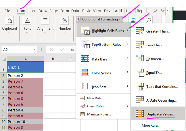
1. Select the range of cells you want to apply the conditional formatting rule to. Then go to Home > Conditional Formatting > Highlight Cell Rules > Duplicate Values.

How to Find and Remove Duplicates in Excel — Conditional formatting

2. Set the “Style” to “Classic” and then “Format only unique or duplicate values”. Don’t forget to leave the drop-down menu to “duplicate”. Finally, choose the formatting style using the “Format with” drop-down menu. Click “OK”.

How to Find and Remove Duplicates in Excel — Conditional formatting remove duplicates

3. You can see how Excel highlights all duplicate values, including the cells. This means that you will need to make sure to only remove rows unless you are actually interested in removing all duplicates.

How to Find and Remove Duplicates in Excel — Highlight duplicates conditional formatting]

In case you want to highlight rows, you can combine all row values in one cell using the =CONCAT formula; if you would like to learn more about this function, read this article on the Microsoft support page.

How to remove duplicates based on one or more columns in Excel?

As a more advanced use of Excel, you can remove duplicates based on one or more columns using Power Query. This feature allows you to select the columns you would like to remove the duplicates from. Let’s explore how to use Power Query to remove duplicates based on one or more columns.

1. Go to Data > Get Data (Power Query).

How to Find and Remove Duplicates in Excel — Power Query

2. Choose “Excel workbook” as your data source.

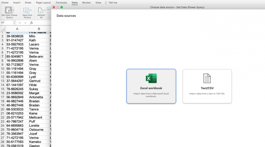
How to Find and Remove Duplicates in Excel — Power Query data source

3. Browse through your files and select the spreadsheet you want to apply the Power Query function to. Click “Next”.

How to Find and Remove Duplicates in Excel — Power Query load data

4. Tick the checkbox next to the worksheet containing your data (located in the left-side menu). Then, click “Load” in the bottom right-hand corner.

How to Find and Remove Duplicates in Excel — Power Query load data

5. As you can see, the dataset has been transformed into a table.

How to Find and Remove Duplicates in Excel — Power Query table

6. Select the columns to apply the Power Query to by pressing Ctrl/Cmd + click on the columns.

How to Find and Remove Duplicates in Excel — Power Query table

7. To delete duplicates, simply click on “Remove Duplicates” in the “Data” tab. Then click “OK” in the pop-up dialog box.

How to Find and Remove Duplicates in Excel — Remove Duplicates

8. Excel will inform you about the number of duplicates removed and how many unique values remain.

How to Find and Remove Duplicates in Excel — Final Alert message

Don’t worry about removing all duplicates, since the dataset you worked on is a copy created by the Power Query function. However, if you want to keep unique values, follow the steps outlined in the sections on the Advanced Filter option or =UNIQUE formula in Excel.

Want to Boost Your Team’s Productivity and Efficiency?

Transform the way your team collaborates with Confluence, a remote-friendly workspace designed to bring knowledge and collaboration together. Say goodbye to scattered information and disjointed communication, and embrace a platform that empowers your team to accomplish more, together.

Key Features and Benefits:

Centralized Knowledge: Access your team’s collective wisdom with ease.
Collaborative Workspace: Foster engagement with flexible project tools.
Seamless Communication: Connect your entire organization effortlessly.
Preserve Ideas: Capture insights without losing them in chats or notifications.
Comprehensive Platform: Manage all content in one organized location.
Open Teamwork: Empower employees to contribute, share, and grow.
Superior Integrations: Sync with tools like Slack, Jira, Trello, and more.

Limited-Time Offer: Sign up for Confluence today and claim your forever-free plan, revolutionizing your team’s collaboration experience.

Conclusion

As we have seen, there are many ways to identify and eliminate duplicates in your data, depending on your needs. Not only can you now successfully organize your data correctly, but removing duplicates makes it easier to identify key patterns and create accurate reports, particularly when working with larger datasets.

Источник

Find Duplicates in Excel

It is very easy to find duplicates in Excel. We can use built in tools (Conditional Formats, Filters) or formula (COUNTIF or VLOOKUP) to find duplicates in Excel Columns or Rows. Let us see the best and easy methods to find duplicate values in Excel.

Find duplicates Using Conditional Formatting

We can easily identify the duplicates using Conditional Formatting Tools in Excel. We can select the range and highlight the duplicate values with color. Following are the different methods to find duplicate entries in excel and strikethrough the duplicates using Conditional Formatting.

Highlighting duplicate values in Excel

We can highlight the duplicate values in the Excel with specific color. We can change the fill color and font color for the duplicate values. Please follow the below steps to identify the duplicates.

Select the required range of cell to find duplicates
Go to ‘Home’ Tab in the Ribbon Menu
Click on the ‘Conditional Formatting’ command
Go to ‘Highlight Cells Rules’ and Click on ‘Duplicate Values…’
And Choose the formatting Options from the drop down list and Click on ‘OK’

Now you can see that all the duplicate values are highlighted as shown in the screen-shot.

Strike through duplicate values in Excel

We can strike through the duplicate values in the Excel. It is very helpful to strike out all duplicate entries in a range of cells. We can use the conditional formatting command in Excel to strike through the duplicate Cells.

Select the required range of cell to strike through the duplicates
Go to ‘Home’ Tab in the Ribbon
Click on the ‘Conditional Formatting’ command
Go to ‘Highlight Cells Rules’ and Click on ‘Duplicate Values…’
And Choose the Custom Format from formatting Options from the drop down list
Select the Strikethrough option from Font effects and Click on ‘OK’

Now you can see that all the duplicate values are stroked out as shown in the screen-shot.

Formula for checking duplicates

We can create formula using COUNTIF or VLOOKUP Functions to check the duplicates in Excel. Following is the step by explanation for finding duplicate values using Excel Formula.

Finding Duplicates using COUNTIF Formula

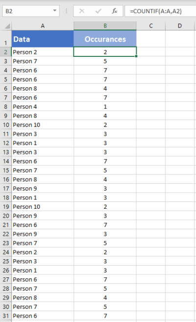
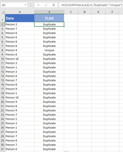
We can use COUNTIF Formula in Excel Cells to identify duplicates in Excel. COUNTIF formula helps to find duplicates in One Column, returns the number of occurrences of a given value. We can identify the duplicates if the Count is greater than 1. We can create new column to mark the duplicates using Excel COUNTIF Formula.

You can see that we have enter the COUNTIF formula in Range B2 to check the total occurrences of A1 value in the entire Column A:A.This will return the frequency of each Cell value of Column A in Column B.

We can identify the duplicate Cells based on the value in the Column B. If the values is greater than 1, we confirm that the values contains duplicate entries in the specified range or column.

Mark Duplicates and Unique Entries using Formula

We can enhance the above formula to mark all duplicates in a Column. The following formula will return ‘Duplicate’ if the cell value contains duplicate values, otherwise returns ‘Unique’.

=IF(COUNTIF(A:A,A2)>1,"Duplicate","Unique")

Formula will return ‘Duplicate’ in the Column B if the value repeats (count >1).

It will return ‘Unique’ in the Column B if the count is 1.

Find duplicate values in excel using VLookup

We can use VLOOKUP formula to compare two columns (or lists) and find the duplicate values. Vlookup helps to find duplicates in Two Column and duplicate rows based on Multiple Columns. Following are steps to find duplicates using VLOOKUP function.

We have two lists in the Excel List 1 in Column A and List 2 in Column B. Let us find the duplicate values in the List 2 which are part of List 1.

=VLOOKUP(B2,$A$2:$A$15,1,FALSE)

VLOOKUP Formula will check for the Cell B2 value in the specified Range (A2:A5) and Returns the value if found, it will return #NA if it is not found in List 1. We can confirm if the the value is duplicated in List 1 and 2 if it returns the Value, it will be unique if it returns #NA.

How to find duplicate values in Excel using VlookUp?

You can use Excel formula to find the duplicate values in Excel by using vlookup formula as described below. You can use the Excel VlookUp to identify the duplicates in Excel.

=IF(ISNA(VLOOKUP(B2,$A$2:$A$15,1,FALSE)),"Unique","Duplicate")

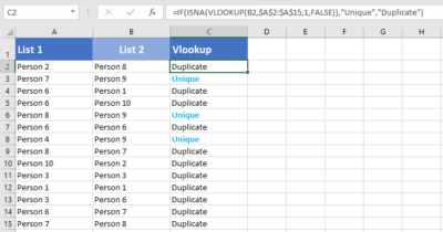
We can enhance this formula to identify the duplicates and unique values in the Column 2. We can use the Excel IF and ISNA Formulas along with VLOOKUP to return the required Labels.

You can use this method to compare with other worksheets and find duplicate values in Different Excel Sheets.

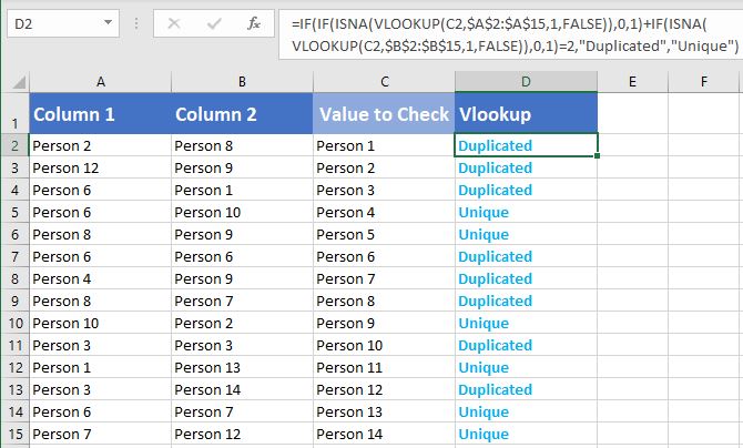
How to find duplicate values in two columns in excel using VlookUp?

Follow the below steps to find the duplicate values in two columns in excel using VlookUp. We generally need this to compare two columns and check if a value is existing in two columns.

=IF(IF(ISNA(VLOOKUP(C2,$A$2:$A$15,1,FALSE)),0,1)
+IF(ISNA(VLOOKUP(C2,$B$2:$B$15,1,FALSE)),0,1)=2,"Duplicated","Unique")

Here, we have Two Target Columns A and B , we check if the items in Column C are duplicated or not.

If you wants to compare two columns and check for values are repeated in both the columns or not, you can use this formula.

Share This Story, Choose Your Platform!

2 Comments

Guru
August 12, 2019 at 7:45 pm — Reply

Thanks for very useful instructions to check duplicates in Excel.
Tom
August 12, 2019 at 7:48 pm — Reply

This is very clear and simple! Thanks a lot for providing clear help to identify the duplicates in Excel.

Page load link

Источник

Duplicate Values | Triplicates | Duplicate Rows

This example teaches you how to find duplicate values (or triplicates) and how to find duplicate rows in Excel.

Duplicate Values

To find and highlight duplicate values in Excel, execute the following steps.

1. Select the range A1:C10.

2. On the Home tab, in the Styles group, click Conditional Formatting.

3. Click Highlight Cells Rules, Duplicate Values.

4. Select a formatting style and click OK.

Result. Excel highlights the duplicate names.

Note: select Unique from the first drop-down list to highlight the unique names.

Triplicates

By default, Excel highlights duplicates (Juliet, Delta), triplicates (Sierra), etc. (see previous image). Execute the following steps to highlight triplicates only.

1. First, clear the previous conditional formatting rule.

2. Select the range A1:C10.

3. On the Home tab, in the Styles group, click Conditional Formatting.

4. Click New Rule.

5. Select ‘Use a formula to determine which cells to format’.

6. Enter the formula =COUNTIF($A$1:$C$10,A1)=3

7. Select a formatting style and click OK.

Result. Excel highlights the triplicate names.

Explanation: =COUNTIF($A$1:$C$10,A1) counts the number of names in the range A1:C10 that are equal to the name in cell A1. If COUNTIF($A$1:$C$10,A1) = 3, Excel formats cell A1. Always write the formula for the upper-left cell in the selected range (A1:C10). Excel automatically copies the formula to the other cells. Thus, cell A2 contains the formula =COUNTIF($A$1:$C$10,A2)=3, cell A3 =COUNTIF($A$1:$C$10,A3)=3, etc. Notice how we created an absolute reference ($A$1:$C$10) to fix this reference.

Note: you can use any formula you like. For example, use this formula =COUNTIF($A$1:$C$10,A1)>3 to highlight names that occur more than 3 times.

Duplicate Rows

To find and highlight duplicate rows in Excel, use COUNTIFS (with the letter S at the end) instead of COUNTIF.

1. Select the range A1:C10.

2. On the Home tab, in the Styles group, click Conditional Formatting.

3. Click New Rule.

4. Select ‘Use a formula to determine which cells to format’.

5. Enter the formula =COUNTIFS(Animals,$A1,Continents,$B1,Countries,$C1)>1

6. Select a formatting style and click OK.

Note: the named range Animals refers to the range A1:A10, the named range Continents refers to the range B1:B10 and the named range Countries refers to the range C1:C10. =COUNTIFS(Animals,$A1,Continents,$B1,Countries,$C1) counts the number of rows based on multiple criteria (Leopard, Africa, Zambia).

Result. Excel highlights the duplicate rows.

Explanation: if COUNTIFS(Animals,$A1,Continents,$B1,Countries,$C1) > 1, in other words, if there are multiple (Leopard, Africa, Zambia) rows, Excel formats cell A1. Always write the formula for the upper-left cell in the selected range (A1:C10). Excel automatically copies the formula to the other cells. We fixed the reference to each column by placing a $ symbol in front of the column letter ($A1, $B1 and $C1). As a result, cell A1, B1 and C1 contain the same formula, cell A2, B2 and C2 contain the formula =COUNTIFS(Animals,$A2,Continents,$B2,Countries,$C2)>1, etc.

7. Finally, you can use the Remove Duplicates tool in Excel to quickly remove duplicate rows. On the Data tab, in the Data Tools group, click Remove Duplicates.

In the example below, Excel removes all identical rows (blue) except for the first identical row found (yellow).

Note: visit our page about removing duplicates to learn more about this great Excel tool.

Источник

Remove duplicate values

Need more help?

Need more help?

How to find duplicate values in Excel?

The example of COUNTIF function and highlighting of the duplicate values

1. Find Duplicates in Excel using Conditional Formatting

2. Find Duplicates in One Column using COUNTIF

3. Filter Duplicates in Excel

Related Queries

CONTENTS:

Find and Highlight Duplicates in Excel

Finding and Highlight Duplicates in a Single Column in Excel

Finding and Highlight Duplicates in Multiple Columns in Excel

Finding and Highlighting Duplicate Rows in Excel

Remove Duplicates in Excel

Remove Duplicates from a Single Column in Excel

Remove Duplicates from Multiple Columns in Excel

Remove Duplicate Rows in Excel

Table of contents

5 Methods to Check & Identify Duplicates in Excel

#1 – Conditional Formatting

#2 – Conditional Formatting (Specific Occurrence)

#3 – Change Rules (Formulas)

#4 – Remove Duplicates

#5 – COUNTIF Formula

Frequently Asked Questions

Recommended Articles

Video Tutorial

What Is A Duplicate Value?

Find And Remove Duplicate Values With The Remove Duplicates Command

Find And Remove Duplicate Values With Advanced Filters

Find And Remove Duplicate Values With A Pivot Table

Find And Remove Duplicate Values With Power Query

Remove Duplicates Based On One Or More Columns

Remove Duplicates Based On The Entire Table

Keep Duplicates Based On A Single Column Or On The Entire Table

Find And Remove Duplicate Values Using A Formula

Find And Remove Duplicate Values With Conditional Formatting

Find And Remove Duplicate Values Using VBA

Conclusions

About the Author

How to find and remove duplicate rows in Excel?

How to Check for Duplicates in Excel?

How to remove duplicates using the Remove Duplicates feature?

How to Combine Multiple Excel Columns Into One?

How to delete duplicates in Excel but keep one?

How to remove duplicates using the Advanced Filter option?

How to remove duplicates using Excel formulae?

How to remove duplicates using conditional formatting?

How to remove duplicates based on one or more columns in Excel?

Want to Boost Your Team’s Productivity and Efficiency?

Conclusion

Find Duplicates in Excel

Find duplicates Using Conditional Formatting

Highlighting duplicate values in Excel

Strike through duplicate values in Excel

Formula for checking duplicates

Finding Duplicates using COUNTIF Formula

Mark Duplicates and Unique Entries using Formula

Find duplicate values in excel using VLookup

How to find duplicate values in Excel using VlookUp?

How to find duplicate values in two columns in excel using VlookUp?

Share This Story, Choose Your Platform!

2 Comments

Duplicate Values

Triplicates

Duplicate Rows