Find differences in excel

Let’s say you have two Excel workbooks, or maybe two versions of the same workbook, that you want to compare. Or maybe you want to find potential problems, like manually-entered (instead of calculated) totals, or broken formulas. You can use Microsoft Spreadsheet Compare to run a report on the differences and problems it finds.

Important: Spreadsheet Compare is only available with Office Professional Plus 2013, Office Professional Plus 2016, Office Professional Plus 2019, or Microsoft 365 Apps for enterprise.

Open Spreadsheet Compare

On the Start screen, click Spreadsheet Compare. If you do not see a Spreadsheet Compare option, begin typing the words Spreadsheet Compare, and then select its option.

In addition to Spreadsheet Compare, you’ll also find the companion program for Access – Microsoft Database Compare. It also requires Office Professional Plus versions or Microsoft 365 Apps for enterprise.

Compare two Excel workbooks

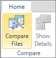
1. Click Home > Compare Files.

   

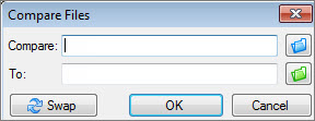
   The Compare Files dialog box appears.

2. Click the blue folder icon next to the Compare box to browse to the location of the earlier version of your workbook. In addition to files saved on your computer or on a network, you can enter a web address to a site where your workbooks are saved.

   

3. Click the green folder icon next to the To box to browse to the location of the workbook that you want to compare to the earlier version, and then click OK.

   Tip: You can compare two files with the same name if they’re saved in different folders.

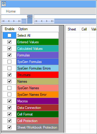
4. In the left pane, choose the options you want to see in the results of the workbook comparison by checking or unchecking the options, such as Formulas, Macros, or Cell Format. Or, just Select All.

   

5. Click OK to run the comparison.

If you get an «Unable to open workbook» message, this might mean one of the workbooks is password protected. Click OK and then enter the workbook’s password. Learn more about how passwords and Spreadsheet Compare work together.

The results of the comparison appear in a two-pane grid. The workbook on the left corresponds to the «Compare» (typically older) file you chose and the workbook on the right corresponds to the «To» (typically newer) file. Details appear in a pane below the two grids. Changes are highlighted by color, depending on the kind of change.

Understanding the results

• In the side-by-side grid, a worksheet for each file is compared to the worksheet in the other file. If there are multiple worksheets, they’re available by clicking the forward and back buttons on the horizontal scroll bar.

  Note: Even if a worksheet is hidden, it’s still compared and shown in the results.

• Differences are highlighted with a cell fill color or text font color, depending on the type of difference. For example, cells with «entered values» (non-formula cells) are formatted with a green fill color in the side-by-side grid, and with a green font in the pane results list. The lower-left pane is a legend that shows what the colors mean.

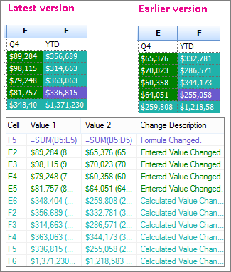
In the example shown here, results for Q4 in the earlier version weren’t final. The latest version of the workbook contains the final numbers in the E column for Q4.

In the comparison results, cells E2:E5 in both versions have a green fill that means an entered value has changed. Because those values changed, the calculated results in the YTD column also changed – cells F2:F4 and E6:F6 have a blue-green fill that means the calculated value changed.

The calculated result in cell F5 also changed, but the more important reason is that in the earlier version its formula was incorrect (it summed only B5:D5, omitting the value for Q4). When the workbook was updated, the formula in F5 was corrected so that it’s now =SUM(B5:E5).

• If the cells are too narrow to show the cell contents, click Resize Cells to Fit.

Excel’s Inquire add-in

In addition to the comparison features of Spreadsheet Compare, Excel 2013 has an Inquire add-in you can turn on that makes an «Inquire» tab available. From the Inquire tab, you can analyze a workbook, see relationships between cells, worksheets, and other workbooks, and clean excess formatting from a worksheet. If you have two workbooks open in Excel that you want to compare, you can run Spreadsheet Compare by using the Compare Files command.

If you don’t see the Inquire tab in Excel, see Turn on the Inquire add-in. To learn more about the tools in the Inquire add-in, see What you can do with Spreadsheet Inquire.

Next steps

If you have «mission critical» Excel workbooks or Access databases in your organization, consider installing Microsoft’s spreadsheet and database management tools. Microsoft Audit and Control Management Server provides powerful change management features for Excel and Access files, and is complemented by Microsoft Discovery and Risk Assessment Server, which provides inventory and analysis features, all aimed at helping you reduce the risk associated with using tools developed by end users in Excel and Access.

Also see Overview of Spreadsheet Compare.

Watch Video – Compare two Columns in Excel for matches and differences

The one query that I get a lot is – ‘how to compare two columns in Excel?’.

This can be done in many different ways, and the method to use will depend on the data structure and what the user wants from it.

For example, you may want to compare two columns and find or highlight all the matching data points (that are in both the columns), or only the differences (where a data point is in one column and not in the other), etc.

Since I get asked about this so much, I decided to write this massive tutorial with an intent to cover most (if not all) possible scenarios.

If you find this useful, do pass it on to other Excel users.

Note that the techniques to compare columns shown in this tutorial are not the only ones.

Based on your dataset, you may need to change or adjust the method. However, the basic principles would remain the same.

If you think there is something that can be added to this tutorial, let me know in the comments section

Compare Two Columns For Exact Row Match

This one is the simplest form of comparison. In this case, you need to do a row by row comparison and identify which rows have the same data and which ones does not.

Example: Compare Cells in the Same Row

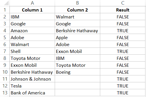
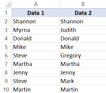
Below is a data set where I need to check whether the name in column A is the same in column B or not.

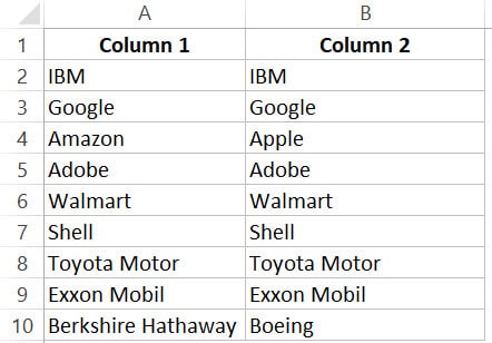
If there is a match, I need the result as “TRUE”, and if doesn’t match, then I need the result as “FALSE”.

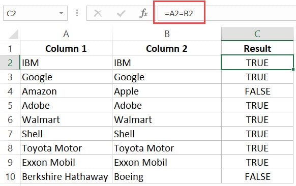
The below formula would do this:

=A2=B2

Example: Compare Cells in the Same Row (using IF formula)

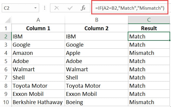
If you want to get a more descriptive result, you can use a simple IF formula to return “Match” when the names are the same and “Mismatch” when the names are different.

=IF(A2=B2,"Match","Mismatch")

Note: In case you want to make the comparison case sensitive, use the following IF formula:

=IF(EXACT(A2,B2),"Match","Mismatch")

With the above formula, ‘IBM’ and ‘ibm’ would be considered two different names and the above formula would return ‘Mismatch’.

Example: Highlight Rows with Matching Data

If you want to highlight the rows that have matching data (instead of getting the result in a separate column), you can do that by using Conditional Formatting.

Here are the steps to do this:

1. Select the entire dataset.
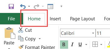
2. Click the ‘Home’ tab.
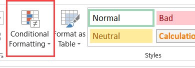
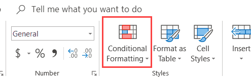
3. In the Styles group, click on the ‘Conditional Formatting’ option.
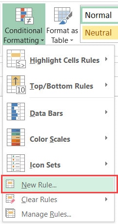
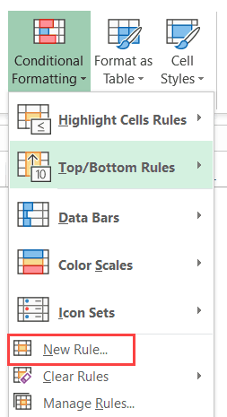
4. From the drop-down, click on ‘New Rule’.
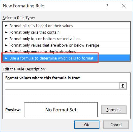
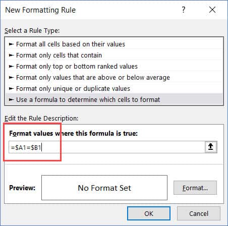
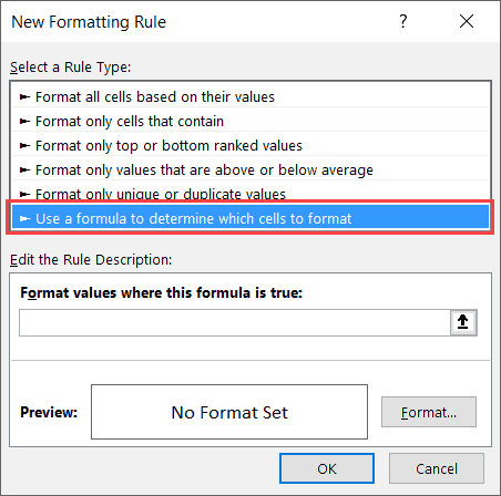
5. In the ‘New Formatting Rule’ dialog box, click on the ‘Use a formula to determine which cells to format’.
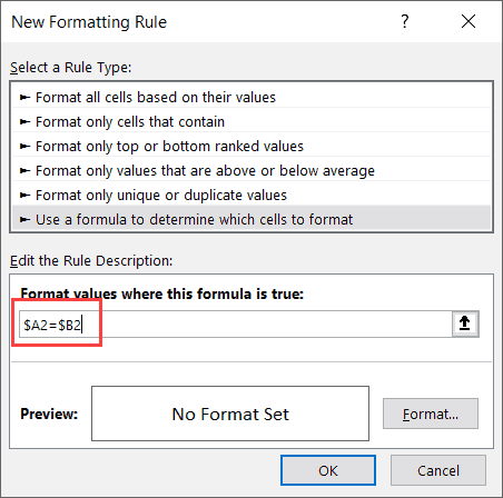
6. In the formula field, enter the formula: =$A1=$B1
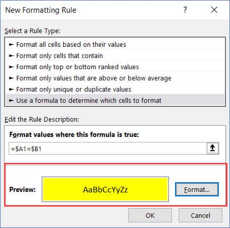
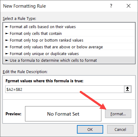
7. Click the Format button and specify the format you want to apply to the matching cells.
8. Click OK.

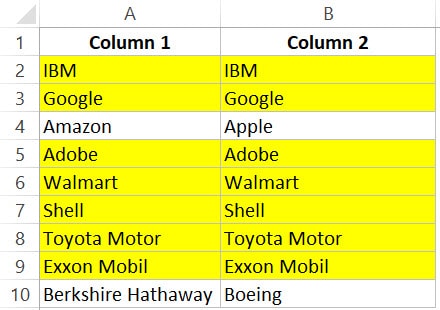
This will highlight all the cells where the names are the same in each row.

Compare Two Columns and Highlight Matches

If you want to compare two columns and highlight matching data, you can use the duplicate functionality in conditional formatting.

Note that this is different than what we have seen when comparing each row. In this case, we will not be doing a row by row comparison.

Example: Compare Two Columns and Highlight Matching Data

Often, you’ll get datasets where there are matches, but these may not be in the same row.

Something as shown below:

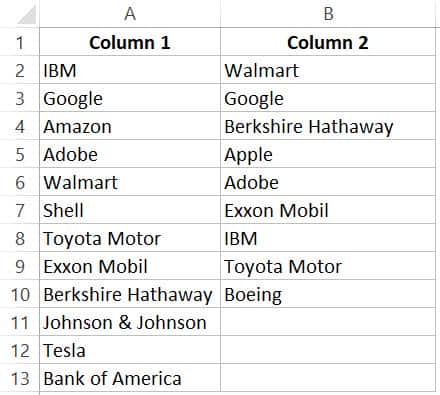
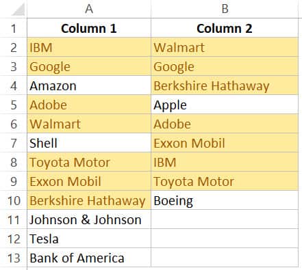
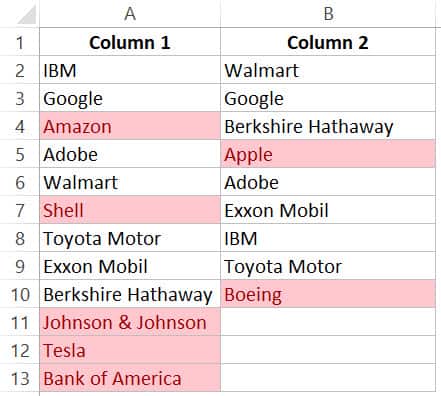
Note that the list in column A is bigger than the one in B. Also some names are there in both the lists, but not in the same row (such as IBM, Adobe, Walmart).

If you want to highlight all the matching company names, you can do that using conditional formatting.

Here are the steps to do this:

1. Select the entire data set.
2. Click the Home tab.
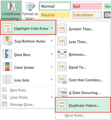
3. In the Styles group, click on the ‘Conditional Formatting’ option.
4. Hover the cursor on the Highlight Cell Rules option.
5. Click on Duplicate Values.
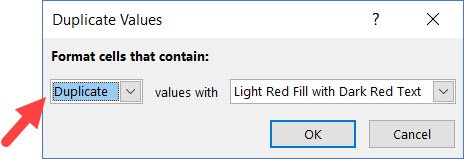
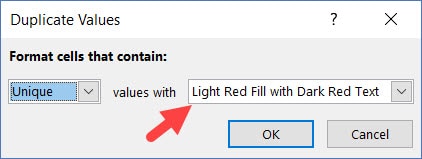
6. In the Duplicate Values dialog box, make sure ‘Duplicate’ is selected.
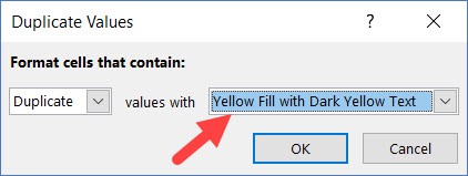
7. Specify the formatting.
8. Click OK.

The above steps would give you the result as shown below.

Note: Conditional Formatting duplicate rule is not case sensitive. So ‘Apple’ and ‘apple’ are considered the same and would be highlighted as duplicates.

Example: Compare Two Columns and Highlight Mismatched Data

In case you want to highlight the names which are present in one list and not the other, you can use the conditional formatting for this too.

1. Select the entire data set.
2. Click the Home tab.
3. In the Styles group, click on the ‘Conditional Formatting’ option.
4. Hover the cursor on the Highlight Cell Rules option.
5. Click on Duplicate Values.
6. In the Duplicate Values dialog box, make sure ‘Unique’ is selected.
7. Specify the formatting.
8. Click OK.

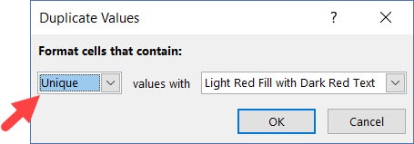
This will give you the result as shown below. It highlights all the cells that have a name that is not present on the other list.

Compare Two Columns and Find Missing Data Points

If you want to identify whether a data point from one list is present in the other list, you need to use the lookup formulas.

Suppose you have a dataset as shown below and you want to identify companies that are present in column A but not in Column B,

To do this, I can use the following VLOOKUP formula.

=ISERROR(VLOOKUP(A2,$B$2:$B$10,1,0))

This formula uses the VLOOKUP function to check whether a company name in A is present in column B or not. If it is present, it will return that name from column B, else it will return a #N/A error.

These names which return the #N/A error are the ones that are missing in Column B.

ISERROR function would return TRUE if there is the VLOOKUP result is an error and FALSE if it isn’t an error.

If you want to get a list of all the names where there is no match, you can filter the result column to get all cells with TRUE.

You can also use the MATCH function to do the same;

=NOT(ISNUMBER(MATCH(A2,$B$2:$B$10,0)))

Note: Personally, I prefer using the Match function (or the combination of INDEX/MATCH) instead of VLOOKUP. I find it more flexible and powerful. You can read the difference between Vlookup and Index/Match here.

Compare Two Columns and Pull the Matching Data

If you have two datasets and you want to compare items in one list to the other and fetch the matching data point, you need to use the lookup formulas.

Example: Pull the Matching Data (Exact)

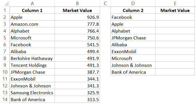
For example, in the below list, I want to fetch the market valuation value for column 2. To do this, I need to look up that value in column 1 and then fetch the corresponding market valuation value.

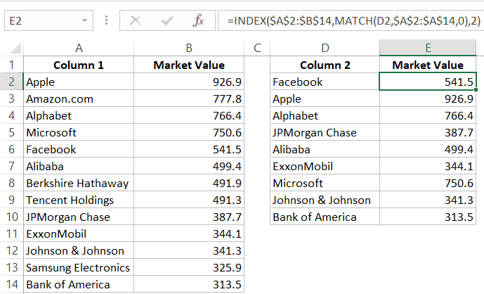
Below is the formula that will do this:

=VLOOKUP(D2,$A$2:$B$14,2,0)

or

=INDEX($A$2:$B$14,MATCH(D2,$A$2:$A$14,0),2)

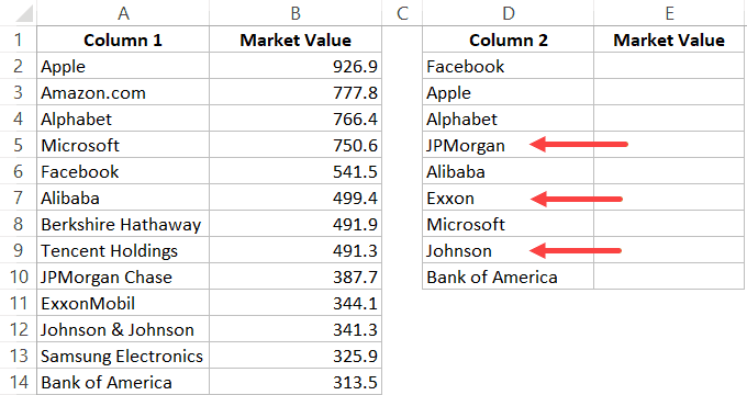
Example: Pull the Matching Data (Partial)

In case you get a dataset where there is a minor difference in the names in the two columns, using the above-shown lookup formulas is not going to work.

These lookup formulas need an exact match to give the right result. There is an approximate match option in VLOOKUP or MATCH function, but that can’t be used here.

Suppose you have the data set as shown below. Note that there are names that are not complete in Column 2 (such as JPMorgan instead of JPMorgan Chase and Exxon instead of ExxonMobil).

In such a case, you can use a partial lookup by using wildcard characters.

The following formula will give is the right result in this case:

=VLOOKUP("*"&D2&"*",$A$2:$B$14,2,0)

or

=INDEX($A$2:$B$14,MATCH("*"&D2&"*",$A$2:$A$14,0),2)

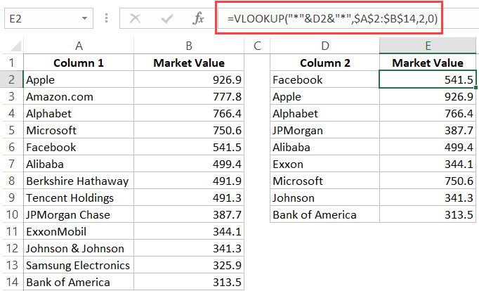
In the above example, the asterisk (*) is a wildcard character that can represent any number of characters. When the lookup value is flanked with it on both sides, any value in Column 1 which contains the lookup value in Column 2 would be considered as a match.

For example, *Exxon* would be a match for ExxonMobil (as * can represent any number of characters).

You May Also Like the Following Excel Tips & Tutorials:

• How to Compare Two Excel Sheets (for differences)
• How to Highlight Blank Cells in Excel.
• How to Compare Text in Excel (Easy Formulas)
• Highlight EVERY Other ROW in Excel.
• Excel Advanced Filter: A Complete Guide with Examples.
• Highlight Rows Based on a Cell Value in Excel
• How to Compare Dates in Excel (Greater/Less Than, Mismatches)

Calculate the difference between two numbers by inputting a formula in a new, blank cell. If A1 and B1 are both numeric values, you can use the “=A1-B1” formula. Your cells don’t have to be in the same order as your formula. For example, you can also use the “=B1-A1” formula to calculate a different value.

How do I find the difference between two columns in Excel?

Compare Two Columns and Highlight Matches

1. Select the entire data set.
2. Click the Home tab.
3. In the Styles group, click on the ‘Conditional Formatting’ option.
4. Hover the cursor on the Highlight Cell Rules option.
5. Click on Duplicate Values.
6. In the Duplicate Values dialog box, make sure ‘Duplicate’ is selected.

What is the formula to find the difference?

When the difference between two values is divided by the average of the same values, a percentage difference calculation has occurred. The formula for percentage difference looks like this: Percentage difference = Absolute difference / Average x 100.

How do I compare two columns in Excel to match?

Excel allows a user to compare two columns by using the SUMPRODUCT function.
Using the SUMPRODUCT to Count Matches Between Two Columns

1. Select cell F2 and click on it.
2. Insert the formula: =SUMPRODUCT(–(B3:B12 = C3:C12))
3. Press enter.

What is an Xlookup in Excel?

Use the XLOOKUP function to find things in a table or range by row.With XLOOKUP, you can look in one column for a search term, and return a result from the same row in another column, regardless of which side the return column is on.

How do you do percentage difference in Excel?

To find the percentage difference in excel, first, find the difference between the two numbers and divide this difference with the base value. After obtaining the results, multiply the decimal number by 100; this result will represent the percentage difference.

How does a Vlookup work?

The VLOOKUP function performs a vertical lookup by searching for a value in the first column of a table and returning the value in the same row in the index_number position. The VLOOKUP function is a built-in function in Excel that is categorized as a Lookup/Reference Function.

How do I count matching values in Excel?

Count cells equal to

1. Generic formula. =COUNTIF(range,value)
2. To count the number of cells equal to a specific value, you can use the COUNTIF function.
3. The COUNTIF function is fully automatic — it counts the number of cells in a range that match the supplied criteria.
4. Excel COUNTIF Function.
5. Excel’s RACON functions.

How do I count matching data in Excel?

How to Count the Total Number of Duplicates in a Column

1. Go to cell B2 by clicking on it.
2. Assign the formula =IF(COUNTIF($A$2:A2,A2)>1,”Yes”,””) to cell B2.
3. Press Enter.
4. Drag down the formula from B2 to B8.
5. Select cell B9.
6. Assign the formula =COUNTIF(B2:B8,”Yes”) to cell B9.
7. Hit Enter.

What is the difference between VLOOKUP and Xlookup?

VLOOKUP data needed to be sorted smallest to largest. However XLOOKUP can perform searches in either direction. XLOOKUP requires referencing fewer cells. VLOOKUP required you to input an entire data set, but XLOOKUP only requires you to reference the relevant columns or rows.

Is Xlookup better than VLOOKUP?

Let’s recap how XLOOKUP outperforms VLOOKUP and INDEX/MATCH: It is the simplest function, with only 3 arguments needed in most cases because the default match_mode is 0 (exact match). It’s a single function, unlike INDEX/MATCH, so it’s faster to type.

How do you find the difference between two percentages?

First Step: find the difference between two percentages, in this case, it’s 15% – 5% = 10%. Second: Take 10 percent, and divide by 2nd percentage: 10/5 = 2. Now multiply this number by 100: 2*100 = 200%. You’re done!

How do I calculate the difference between two negative numbers in Excel?

The percentage difference between the two numbers in Excel

1. The difference between numbers A2 and B2 (A2-B2) can be negative. So, we have used the ABS() function (ABS(A2-B2)) to make the number absolute.
2. Then we have multiplied the absolute value by 2 and then divided the value by (A2+B2)

How do you do a VLOOKUP for beginners?

1. In the Formula Bar, type =VLOOKUP().
2. In the parentheses, enter your lookup value, followed by a comma.
3. Enter your table array or lookup table, the range of data you want to search, and a comma: (H2,B3:F25,
4. Enter column index number.
5. Enter the range lookup value, either TRUE or FALSE.

How use VLOOKUP formula in Excel with example?

This is the default method if you don’t specify one. For example, =VLOOKUP(90,A1:B100,2,TRUE). Exact match – 0/FALSE searches for the exact value in the first column. For example, =VLOOKUP(“Smith”,A1:B100,2,FALSE).

How do you count cells that match?

Match one criterion exactly — COUNTIF

1. Select the cell in which you want to see the count (cell A12 in this example)
2. Type an equal sign (=) to start the formula.
3. Type: COUNTIF(
4. Select the cells that contain the values to check for the criterion.
5. Type a comma, to separate the arguments.
6. Type the criterion.

How do I compare a range of values in Excel?

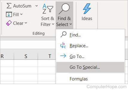
To quickly highlight cells with different values in each individual row, you can use Excel’s Go To Special feature.

1. Select the range of cells you want to compare.
2. On the Home tab, go to Editing group, and click Find & Select > Go To Special… Then select Row differences and click the OK button.

How do you use match and count?

If you want to count rows where two (or more) criteria match, you can use a formula based on the COUNTIFS function. The COUNTIFS function takes multiple criteria in pairs — each pair contains one range and the associated criteria for that range. To generate a count, all conditions must match.

How do I create an Xlookup in Excel?

INSTALLING THE XLOOKUP ADDIN [GKXLOOKUP]

1. OPEN EXCEL.
2. Go to OPTIONS>ADDINS.
3. Select EXCEL ADD-INS.
4. Click GO.
5. A new dialog box will open as shown in the picture containing all the EXCEL ADD-INS list.
6. We can select the Addins we want to activate.
7. In our case we want to install the add in , so click BROWSE.

How do I enable Xlookup in Excel?

1. Position the cell cursor in cell E4 of the worksheet.
2. Click the Lookup & Reference option on the Formulas tab followed by XLOOKUP near the bottom of the drop-down menu to open its Function Arguments dialog box.
3. Click cell D4 in the worksheet to enter its cell reference into the Lookup_value argument text box.

What version of Excel is Xlookup available?

Office 365
What Versions of Excel Will Have XLOOKUP? Only Excel for Office 365 will get the new XLOOKUP function. Excel 2019 and all previous versions won’t ever get this new function.

When you’re working with data in Excel, sooner or later you will have to compare data. This could be comparing two columns or even data in different sheets/workbooks.

In this Excel tutorial, I will show you different methods to compare two columns in Excel and look for matches or differences.

There are multiple ways to do this in Excel and in this tutorial I will show you some of these (such as comparing using VLOOKUP formula or IF formula or Conditional formatting).

So let’s get started!

Compare Two Columns (Side by Side)

This is the most basic type of comparison where you need to compare a cell in one column with the cell in the same row in another column.

Suppose you have a dataset as shown below and you simply want to check whether the value in column A in a specific cell is the same (or different) when compared with the value in the adjacent cell.

Of course, you can do this when you have a small dataset when you have a large one, you can use a simple comparison formula to get this done. And remember, there is always a chance of human error when you do this manually.

So let me show you a couple of easy ways to do this.

Compare Side by Side Using the Equal to Sign Operator

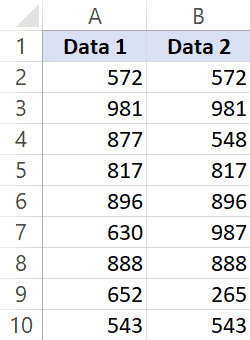
Suppose you have the below dataset and you want to know what rows have the matching data and what rows have different data.

Below is a simple formula to compare two columns (side by side):

=A2=B2

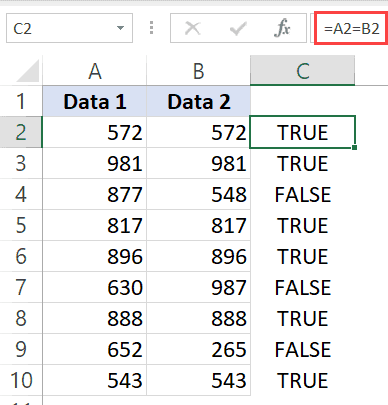
The above formula will give you a TRUE if both the values are the same and FALSE in case they are not.

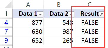
Now, if you need to know all the values that match, simply apply a filter and only show all the TRUE values. And if you want to know all the values that are different, filter all the values that are FALSE (as shown below):

When using this method to do column comparison in Excel, it’s always best to check that your data does not have any leading or trailing spaces. If these are present, despite having the same value, Excel will show them as different. Here is a great guide on how to remove leading and trailing spaces in Excel.

Compare Side by Side Using the IF Function

Another method that you can use to compare two columns can be by using the IF function.

This is similar to the method above where we used the equal to (=) operator, with one added advantage. When using the IF function, you can choose the value you want to get when there are matches or differences.

For example, if there is a match, you can get the text “Match” or can get a value such as 1. Similarly, when there is a mismatch, you can program the formula to give you the text “Mismatch” or give you a 0 or blank cell.

Below is the IF formula that returns ‘Match’ when the two cells have the cell value and ‘Not a Match’ when the value is different.

=IF(A2=B2,"Match","Not a Match")

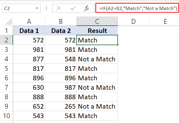
The above formula uses the same condition to check whether the two cells (in the same row) have matching data or not (A2=B2). But since we are using the IF function, we can ask it to return a specific text in case the condition is True or False.

Once you have the formula results in a separate column, you can quickly filter the data and get rows that have the matching data or rows with mismatched data.

Also read: Does Not Equal Operator in Excel (Examples)

Highlight Rows with Matching Data (or Different Data)

Another great way to quickly check the rows that have matching data (or have different data), is to highlight these rows using conditional formatting.

You can do both – highlight rows that have the same value in a row as well as the case when the value is different.

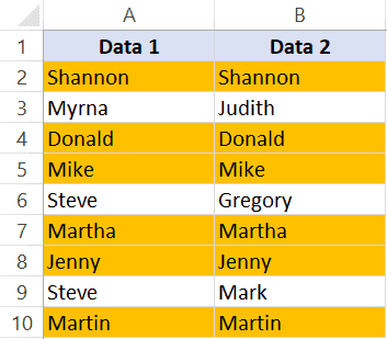
Suppose you have a dataset as shown below and you want to highlight all the rows where the name is the same.

Below are the steps to use conditional formatting to highlight rows with matching data:

1. Select the entire dataset (except the headers)
2. Click the Home tab
3. In the Styles group, click on Conditional Formatting
4. In the options that show up, click on ‘New Rule’
5. In the ‘New Formatting Rule’ dialog box, click on the option -”Use a formula to determine which cells to format’
6. In the ‘Format values where this formula is true’ field, enter the formula: =$A2=$B2
7. Click on the Format button
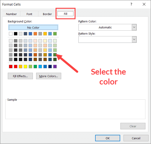
8. Click on the ‘Fill’ tab and select the color in which you want to highlight the rows with the same value in both columns
9. Click OK

The above steps would instantly highlight the rows where the name is the same in both columns A and B (in the same row). And in the case where the name is different, those rows will not be highlighted.

In case you want to compare two columns and highlight rows where the names are different, use the below formula in the conditional formatting dialog box (in step 6).

=$A2<>$B2

How does this work?

When we use conditional formatting with a formula, it only highlights those cells where the formula is true.

When we use $A2=$B2, it will check each cell (in both columns) and see whether the value in a row in column A is equal to the one in column B or not.

In case it’s an exact match, it will highlight it in the specified color, and in case it doesn’t match, it will not.

The best part about conditional formatting is that it doesn’t require you to use a formula in a separate column. Also, when you apply the rule on a dataset, it remains dynamic. This means that if you change any name in the dataset, conditional formatting will accordingly adjust.

Compare Two Columns Using VLOOKUP (Find Matching/Different Data)

In the above examples, I showed you how to compare two columns (or lists) when we are just comparing side by side cells.

In reality, this is rarely going to be the case.

In most cases, you will have two columns with data and you would have to find out whether a data point in one column exists in the other column or not.

In such cases, you can’t use a simple equal-to sign or even an IF function.

You need something more powerful…

… something that’s right up VLOOKUP’s alley!

Let me show you two examples where we compare two columns in Excel using the VLOOKUP function to find matches and differences.

Compare Two Columns Using VLOOKUP and Find Matches

Suppose we have a dataset as shown below where we have some names in columns A and B.

If you have to find out what are the names that are in column B that are also in column A, you can use the below VLOOKUP formula:

=IFERROR(VLOOKUP(B2,$A$2:$A$10,1,0),"No Match")

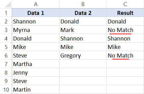
The above formula compares the two columns (A and B) and gives you the name in case the name is in column B as well A, and it returns “No Match” in case the name is in Column B and not in Column A.

By default, the VLOOKUP function will return a #N/A error in case it doesn’t find an exact match. So to avoid getting the error, I have wrapped the VLOOKUP function in the IFERROR function, so that it gives “No Match” when the name is not available in column A.

You can also do the other way round comparison – to check whether the name is in Column A as well as Column B. The below formula would do that:

=IFERROR(VLOOKUP(A2,$B$2:$B$6,1,0),"No Match")

Compare Two Columns Using VLOOKUP and Find Differences (Missing Data Points)

While in the above example, we checked whether the data in one column was there in another column or not.

You can also use the same concept to compare two columns using the VLOOKUP function and find missing data.

Suppose we have a dataset as shown below where we have some names in columns A and B.

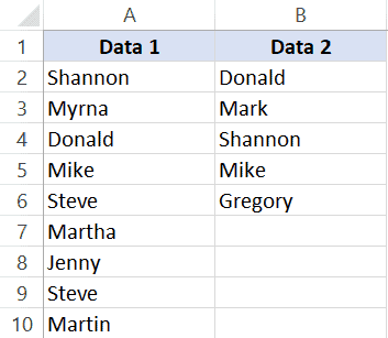
If you have to find out what are the names that are in column B that not there in column A, you can use the below VLOOKUP formula:

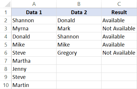
=IF(ISERROR(VLOOKUP(B2,$A$2:$A$10,1,0)),"Not Available","Available")

The above formula checks the name in column B against all the names in Column A. In case it finds an exact match, it would return that name, and in case it doesn’t find and exact match, it will return the #N/A error.

Since I am interested in finding the missing names that are there is column B and not in column A, I need to know the names that return the #N/A error.

This is why I have wrapped the VLOOKUP function in the IF and ISERROR functions. This whole formula gives the value – “Not Available” when the name is missing in Column A, and “Available” when it’s present.

To know all the names that are missing, you can filter the result column based on the “Not Available” value.

You can also use the below MATCH function to get the same result:

=IF(ISNUMBER(MATCH(B2,$A$2:$A$10,0)),"Available","Not Available")

Common Queries when Comparing Two Columns

Below are some common queries I usually get when people are trying to compare data in two columns in Excel.

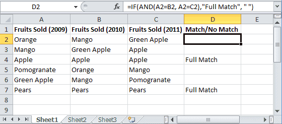
Q1. How to compare multiple columns in Excel in the same row for matches? Count the total duplicates also.

Ans. We have given the procedure to compare two columns in excel for the same row above. But if you want to compare multiple columns in excel for the same row then see the example

=IF(AND(A2=B2, A2=C2),"Full Match", "")

Here we have compared data of column A, column B, and column C. After this, I have applied the above formula in column D and get the result.

Now to count the duplicates, you need to use the Countif function.

=IF(COUNTIF($A2:$E2, $A2)=5, "Full Match", "")

Q2. Which operator do you use for matches and differences?

Ans. Below are the operators to use:

• To find matches, use the equal to sign (=)
• To find differences (mismatches), use the not-equal-to sign (<>)

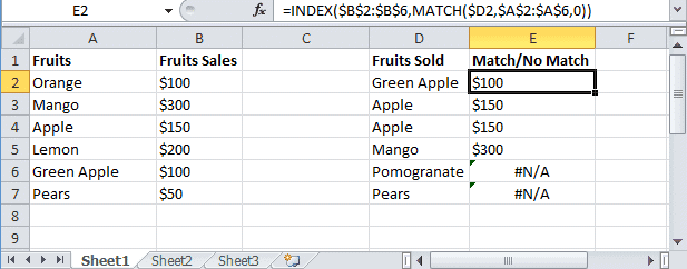
Q3. How to compare two different tables and pull matching data?

Ans. For this, you can use the VLOOKUP function or INDEX & MATCH function. To understand this thing in a better way we will take an example.

Here we will take two tables and now want to do pull matching data. In the first table, you have a dataset and in the second table, take the list of fruits and then use pull matching data in another column. For pull matching, use the formula

=INDEX($B$2:$B$6,MATCH($D2,$A$2:$A$6,0))

Q4. How to remove duplicates in Excel?

Ans. To remove duplicate data you need to first find the duplicate values.

To find the duplicate, you can use various methods like conditional formatting, Vlookup, If Statement, and many more. Excel also has an in-built tool where you can just select the data, and remove the duplicates from a column or even multiple columns

Q5. I can see that there is a matching value in both columns. However, the formulas you have shared above are not considering these as exact matches. Why?

Ans: Excel considers something an exact match when each and every character of one cell is equal to the other. There is a high chance that in your dataset there are leading or trailing spaces.

Although these spaces may still make the values seem equal to a naked eye, for Excel these are different. If you have such a dataset, it’s best to get rid of these spaces (you can use Excel functions such as TRIM for this).

Q7. How to compare two columns that give the result as TRUE when all first columns’ integer values are not less than the second column’s integer values. To solve this problem, I do not require conditional formatting, Vlookup function, If Statement, and any other formulas. I need the formula to solve this problem.

Ans. You can use the array formula for solving this problem.

The syntax is {=AND(H6:H12>I6:I12)}. This will give you “True” as a result whenever the value of Column H is greater than the value in column I else “False” will be the result.

You may also like the following Excel tutorials:

• Compare Two Columns in Excel (for matches and differences)
• How to Remove Blank Columns in Excel? (Formula + VBA)
• How to Hide Columns Based On Cell Value in Excel
• How to Split One Column into Multiple Columns in Excel
• How to Select Alternate Columns in Excel (or every Nth Column)
• How to Paste in a Filtered Column Skipping the Hidden Cells
• Best Excel Books (that will make you an Excel Pro)
• How to Flip Data in Excel (Columns, Rows, Tables)?
• Find the Closest Match in Excel (Nearest Value)
• How to Compare Two Cells in Excel?
• VLOOKUP Not Working – 7 Possible Reasons + How to Fix!

Updated: 02/01/2021 by

To find the differences between two columns of data in a Microsoft Excel spreadsheet, select your version of Excel, and follow the instructions.

Microsoft Excel for Office 365

1. Open the Excel spreadsheet containing the data you want to compare.
2. Select all the cells in both columns containing the data to be compared.

• How to select one or more cells in a spreadsheet program.

1. In the Ribbon, on the Home tab, find the Editing section and click Find & Select.
2. In the drop-down menu, select Go To Special.

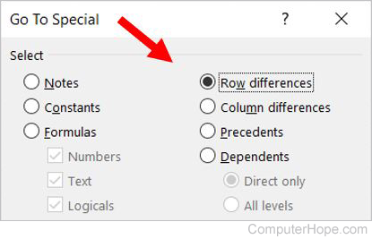
1. In the Go To Special pop-up window, click Row differences, then click OK. Excel selects the differences between the two columns.

1. To highlight these differences, leave them selected, and click the paint bucket icon in the font menu and select the color you want to use. Similarly, you can right-click and select the paint bucket to highlight the cells.

Tip

You can use the shortcut Ctrl+G, then click Special to open the Go To menu. Alternatively, press F5, then click Special on the pop-up screen.

Microsoft Excel 2007 & 2010

1. Open the Excel spreadsheet containing the data you want to compare.
2. Select all the cells in both columns containing the data to be compared.

• How to select one or more cells in a spreadsheet program.

1. In the Ribbon, on the Home tab, go to Find & Select, then click Go To.
2. In the Go To pop-up window, click Row differences, then click OK. Excel selects the difference between the two columns.
3. To highlight these differences, leave them selected, and click the paint bucket icon in the font menu and select the color you want to use. Similarly, you can right-click and select the paint bucket to highlight the cells.

Microsoft Excel 2003

1. Open the Excel spreadsheet containing the data you want to compare.
2. Select all the cells in both columns containing the data to be compared.

• How to select one or more cells in a spreadsheet program.

1. In the file menu at the top of the program window, click Edit and select Go To.
2. In the Go To Special pop-up window, click Row differences, then click OK. Excel selects the difference between the two columns.
3. To highlight these differences, leave them selected, and click the paint bucket icon in the font menu and select the color you want to use. Similarly, you can right-click and select the paint bucket to highlight the cells.