Find data from excel

When you need to find and extract a column of data from one table and place it in another, use the VLOOKUP function. This function works in any version of Excel in Windows and Mac, and also in Google Sheets. It allows you to find data in one table using some identifier it has in common with another table. The two tables can be on different sheets or even on different workbooks. There is also an HLOOKUP function, which does the same thing, but with data arranged horizontally, across rows.

The MATCH and INDEX functions are good to use when you’re concerned with the location of specific data, such as the column or row that contains a person’s name. 

Premium Options

Before we get into the Excel functions, did you know that Envato Market has a range of Excel scripts and plugins that let you perform advanced functions? 

Screencast

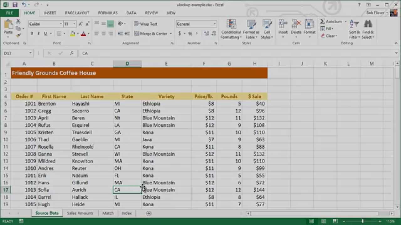
If you want to follow along with this tutorial using your own Excel file, you can do so. Or if you prefer, download the zip file included for this tutorial, which contains a sample workbook called vlookup example.xlsx.

Using VLOOKUP

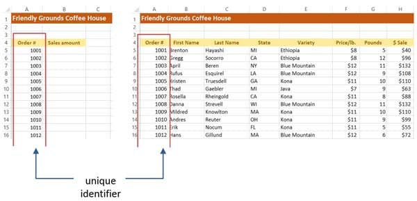
When VLOOKUP finds the identifier that you specify in the source data, it can then find any cell in that row and return the information to you. Note that in the source data, the identifier must be in the first column of the table.

Syntax

The syntax of the VLOOKUP function is:

=VLOOKUP(lookup value, table range, column number, [true/false])

Here’s what these arguments mean:

• Lookup value. The cell that has the unique identifier.
• Table range. The range of cells that has the identifier in the first column, followed by the rest of the data in the other columns.
• Column number. The number of the column that has the data you’re looking for. Don’t get that confused with the column’s letter. In the above illustration, the states are in column 4.
• True/False. This argument is optional. True means that an approximate match is acceptable, and False means that only an exact match is acceptable.

We want to find sales amounts from the table in the illustration above, so we use these arguments:

Define a Range Name to Create an Absolute Reference

In Vlookup example.xlsx, look at the Sales Amounts worksheet. We’ll enter the formula in B5, then use the AutoFill feature to copy the formula down the sheet. That means the table range in the formula has to be an absolute reference. A good way to do that is to define a name for the table range.

Defining a Range Name in Excel

1. Before entering the formula, go to the source data worksheet.
2. Select all the cells from A4 (header for the Order # column) down through H203. A quick way of doing it is to click A4, then press Ctrl-Shift-End (Command-Shift-End on the Mac).
3. Click inside the Name Box above column A (the Name Box now displays A4).
4. Type data, then press Enter.
5. You can now use the name data in the formula instead of $A$4:$H$203.

Defining a Range name in Google Sheets

In Google Sheets, defining a name is a little different.

1. Click the first column header of your source data, then press Ctrl-Shift-Right Arrow (Command-Shift-Right Arrow on the Mac). That selects the row of column headers.
2. Press Ctrl-Shift-Down Arrow (Command-Shift-Down Arrow on the Mac). That selects the actual data.
3. Click the Data menu, then select Named and protected ranges.
4. In the Name and protected ranges box on the right, type data, then click Done.

Entering the Formula

To enter the formula, go to the Sales Amounts worksheet and click in B5.

Enter the formula:

=VLOOKUP(A5,data,8,FALSE)

Press Enter.

The result should be 40. To fill in the values down the column, click back on B5, if necessary. Put the mouse pointer on the AutoFill dot in the cell’s lower-right corner, so the mouse pointer becomes a cross hair.

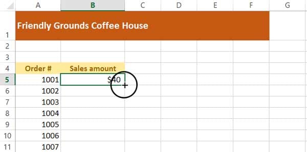
Double-click to fill the values down the column.

If you want, you can run the VLOOKUP function in the next few columns to extract other fields, like last name or state.

Using MATCH

The MATCH function is doesn’t return the value of data to you; you provide the value that you’re looking for, and the function returns the position of that value. It’s like asking where is #135 Main Street, and getting the answer that it’s the 4^th building down the street.

Syntax

The syntax of the MATCH function is:

=MATCH(lookup value, table range, [match type])

The arguments are:

• Lookup value. The cell that has the unique identifier.
• Table range. The range of cells you’re searching.
• Match type. Optional. It’s how you specify how close of a match you want, as follows:

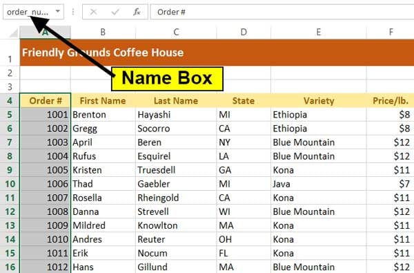
As with the VLOOKUP function, you’ll probably find the MATCH function easier to use if you apply a range name. Go to the Source Data sheet, select from B4 (column header for order #) to the bottom, click in the Name box above column A, and call it order_number. Note that the values are in ascending order.

Go to the Match tab of the worksheet. In B5, enter the MATCH function:

=MATCH(A5,order_number,1)

If you didn’t define a range name, you’d write the function as:

=MATCH(A5,'Source
Data'!A5:A203,0)

Either way, you can see that this is in the 14th position (making it the 13^th order).

Using INDEX

The INDEX function is the opposite of the MATCH function and is similar to VLOOKUP. You tell the function what row and column of the data you want, and it tells you the value of what’s in the cell.

Syntax

The syntax of the INDEX function is:

=INDEX(data range, row number, [column number])

The arguments are:

• Data range. Just like the other two functions, this is the table of data.
• Row number. The row number of the data, which is not necessarily the row of the worksheet. If the table range starts on row 10 of the sheet, then that’s row #1.
• Column number. The column number of the data range. If the range starts on column E, that’s column #1.

Excel’s documentation will tell you that the column number argument is optional, but the row number is sort of optional, too. If the table range has only one row or one column, you don’t have to use the other argument.

Go to the Index sheet of the workbook and click in C6. We first want to find what’s contained in row 9, column 3 of the table. In the formula, we’ll use the range name that we created earlier.

Enter the formula:

=INDEX(data,A6,B6)

It returns a customer’s last name: Strevell. Change the values of A6 and B6, and the result in C6 will show different results (note that many rows have the same states and product names).

Conclusion

The ability of a worksheet to look at another worksheet and extract data is a great tool. This way, you can have one sheet that contains all the data you need for many purposes, then extract what you need for specific instances. 

When people save data in the JSON or CSV format, they’re intending for that data to be accessed programmatically. But much of the world’s data is stored in spreadsheet files, and many of those files are in the Excel format. Excel is used because people can manipulate it easily, and it’s a powerful tool in its own right. However, there is a lot of automation that can be done by extracting data from a spreadsheet, and this process also allows you to bring data from multiple kinds of sources into one program.

We’ll first take a quick look at how to save an Excel file as a CSV file. This is sometimes the quickest and easiest way to extract data. But it’s a manual process, so you’d have to open the file in Excel and save it as a CSV again every time the file is updated. It’s much better in many situations to just extract the data from Excel directly.

The example we’ll use is the data you can download from Mapping Police Violence. If you can’t download this file from the site for some reason, you can also find a snapshot of this spreadsheet from 6/19/20 in the beyond_pcc/social_justice_datasets/ directory of the online resources for Python Crash Course.

• Converting an Excel File to CSV
• Installing openpyxl
• Opening an Excel File
• Accessing Data in a Worksheet
• Accessing Data from Cells
• Extracting Data from Specific Cells
• Refactoring
• Further Reading

Converting an Excel File to CSV

You can create a CSV file from any single worksheet in an Excel workbook. To do this, first click on the tab for the worksheet you want to focus on. Then choose File > Save As, and in the File Format dropdown choose CSV UTF-8 (Comma-delimited) (.csv). You’ll get a message that the entire workbook can’t be saved in this format, but if you click OK you’ll get a copy of the current worksheet in CSV format.

To look at the file and make sure it contains the data you expect it to, locate the new CSV file in a file browser and open it with a text editor. If you open the file with a spreadsheet application like Excel, it won’t look any different than a regular Excel file.

top

Installing openpyxl

We’ll be using the openpyxl library to access the data in an Excel file. You can install this library with pip:

$ pip install --user openpyxl

top

Opening an Excel File

To follow along with this tutorial, make a folder somewhere on your system called extracting_from_excel. Make a data folder inside this directory; it’s a good idea to keep your data files in their own directory. I saved the file mapping_police_violence_snapshot_061920.xlsx in my data directory; you can work with this file, or any .xls or .xlsx file you’re interested in.

The following code will open the Excel file and print the names of all worksheets in the file:

from openpyxl import load_workbook

data_file = 'data/mapping_police_violence_snapshot_061920.xlsx'

# Load the entire workbook.
wb = load_workbook(data_file)

# List all the sheets in the file.
print("Found the following worksheets:")
for sheetname in wb.sheetnames:
    print(sheetname)

First we import the load_workbook() function, and assign the path to the data file to data_file. Then we call load_workbook() with the correct path, and assign the returned object, representing the entire workbook, to wb. You’ll see this convention in the documentation for openpyxl.

The names of all worksheets in the file are stored in the sheetnames attribute. Here’s the output for this data file:

Found the following worksheets:
2013-2019 Police Killings
2013-2019 Killings by PD
2013-2019 Killings by State
Police Killings of Black Men

top

Accessing Data in a Worksheet

We want to access the actual data in a specific worksheet. To do this we grab the worksheet we’re interested in, and then extract the data from all rows in the worksheet:

from openpyxl import load_workbook

data_file = 'data/mapping_police_violence_snapshot_061920.xlsx'

# Load the entire workbook.
wb = load_workbook(data_file)

# Load one worksheet.
ws = wb['2013-2019 Killings by State']
all_rows = list(ws.rows)

print(f"Found {len(all_rows)} rows of data.")

print("nFirst rows of data:")
for row in all_rows[:5]:
    print(row)

Worksheets are accessed by name through the workbook object. Here we assign a worksheet to ws. Once you have a worksheet object, you can access all the rows through the ws.rows attribute. This attribute is a generator, a Python object that efficiently returns one item at a time from a collection. We can convert this to the more familar list using the list() function. Here we create a list of all the rows in the workbook. We then print a message about how many rows were found, and print the first few rows of data:

Found 55 rows of data.

First rows of data:
(<Cell '2013-2019 Killings by State'.A1>, <Cell...
(<Cell '2013-2019 Killings by State'.A2>, <Cell...
(<Cell '2013-2019 Killings by State'.A3>, <Cell...

In this worksheet, we found 55 rows of data. Each row of data is made up of a series of cell objects.

top

Accessing Data from Cells

So far we have accessed the Excel file, an individual worksheet, and a series of rows. Now we can access the actual data in the cells.

To begin with, we’ll look at just the data in the first row:

from openpyxl import load_workbook

data_file = 'data/mapping_police_violence_snapshot_061920.xlsx'

# Load the entire workbook.
wb = load_workbook(data_file)

# Load one worksheet.
ws = wb['2013-2019 Killings by State']
all_rows = list(ws.rows)

for cell in all_rows[0]:
    print(cell.value)

We loop through all cells in the row, and print the value of each cell. This is accessed through the value attribute of the cell object.

State
Population
African-American Alone
% African-American
% Victims Black
Disparity
--snip--

top

The previous example is helpful, perhaps, when looking at a list of headings for a worksheet over a remote connection. But usually when we’re analyzing the data from a spreadsheet we can just open the file in Excel, look for the information we want, and then write code to extract that information. We usually aren’t interested in every single cell in a row, though. We’re often interested in selected cells in every row in the sheet.

The following example pulls data from three specific columns in each row in the file containing the data we’re interested in:

from openpyxl import load_workbook

data_file = 'data/mapping_police_violence_snapshot_061920.xlsx'

# Load the entire workbook.
wb = load_workbook(data_file)

# Load one worksheet.
ws = wb['2013-2019 Killings by State']
all_rows = list(ws.rows)

# Pull information from specific cells.
for row in all_rows[1:52]:
    state = row[0].value
    percent_aa = row[3].value
    percent_aa_victims = row[4].value

    print(f"{state}")
    print(f" {percent_aa}% of residents are African American")
        print(f" {percent_aa_victims}% killed by police were African American")

Here we loop through the all of the rows that contain the states’ data. For each row, we pull the values at index 0, 3, and 4, and assign each of these to an appropriate variable name. We then print a statement summarizing what these values mean.

The output isn’t quite what we expect:

Alabama
 =C2/B2% of residents are African American
 =G2/N2% killed by police were African American

Alaska
 =C3/B3% of residents are African American
 =G3/N3% killed by police were African American

Arizona
 =C4/B4% of residents are African American
 =G4/N4% killed by police were African American

--snip--

The values in these cells are actually formulas. If we want the values computed from these formulas, we need to pass the data_only=True flag when we load the workbook:

from openpyxl import load_workbook

data_file = 'data/mapping_police_violence_snapshot_061920.xlsx'

# Load the entire workbook.
wb = load_workbook(data_file, data_only=True)

# Load one worksheet.
ws = wb['2013-2019 Killings by State']
all_rows = list(ws.rows)

# Pull information from specific cells.
for row in all_rows[1:52]:
    state = row[0].value
    percent_aa = row[3].value
    percent_aa_victims = row[4].value

    print(f"n{state}")
    print(f" {percent_aa}% of residents are African American")
    print(f" {percent_aa_victims}% killed by police were African American")

Now we see output that’s much more like what we were expecting:

Alabama
 0.2617950029039261% of residents are African American
 0.37681159420289856% killed by police were African American

Alaska
 0.032754132106314705% of residents are African American
 0.12195121951219512% killed by police were African American

Arizona
 0.04052054304611518% of residents are African American
 0.09037900874635568% killed by police were African American

--snip--

Data analysis almost always involves some degree of reformatting. For this output, we’ll round the percentages to two decimal places, and turn them into neatly-formatted integers for display:

# Pull information from specific cells.
for row in all_rows[1:52]:
    state = row[0].value
    percent_aa = int(round(row[3].value, 2) * 100)
    percent_aa_victims = int(round(row[4].value, 2) * 100)

Here’s the cleaner output:

Alabama
 26% of residents are African American
 38% killed by police were African American

Alaska
 3% of residents are African American
 12% killed by police were African American

Arizona
 4% of residents are African American
 9% killed by police were African American

--snip--

Be careful about rounding data during the processing phase. If you were going to pass this data to a plotting library, you probably want to do the rounding in the plotting code. This can affect your visualization. For example if two percentages round to the same value in two decimal places but they’re different in the third decimal place, you’ll lose the ability to sort items precisely. In this situation, it’s important to ask whether the third decimal place is meaningful or not.

Also, note that you will often need to identify the specific rows that need to be looped over. Spreadsheets are nice and structured, but people are also free to write anything they want in any cell. Many spreadsheets have some notes in a few cells after all the rows of data. These can be notes about sources of the raw data, dates of data collection, authors, and more. You will probably need to exclude these rows, either by looping over a slice as shown here, or using a try/except block to only extract data if the operation for each row is successful.

Finally, you should be aware that people can modify the hard-coded values in a spreadsheet without updating the values derived from formulas that use those values. If you have any doubt about whether the spreadhseet you’re working from has been updated, you should re-run the formulas yourself before using the data_only=True flag when loading a workbook.

top

Refactoring

That’s probably enough to get you started working with data that’s stored in Excel files, but it’s worth showing a bit of refactoring on the program we’ve been using in this tutorial. Here’s what the code looks like at this point:

from openpyxl import load_workbook

data_file = 'data/mapping_police_violence_snapshot_061920.xlsx'

# Load the entire workbook.
wb = load_workbook(data_file, data_only=True)

# Load one worksheet.
ws = wb['2013-2019 Killings by State']
all_rows = list(ws.rows)

# Pull information from specific cells.
for row in all_rows[1:5]:
    state = row[0].value
    percent_aa = int(round(row[3].value, 2) * 100)
    percent_aa_victims = int(round(row[4].value, 2) * 100)

    print(f"n{state}")
    print(f" {percent_aa}% of residents are African American")
    print(f" {percent_aa_victims}% killed by police were African American")

If all we wanted to do was generate a text summary of this data, this code would probably be fine. But we’re probably going to do some visualization work, and maybe we want to bring in some additional data from another file. If we’re going to do anything further, it’s worth breaking this into a couple functions. Here’s how we might organize this code:

from openpyxl import load_workbook


def get_all_rows(data_file, worksheet_name):
    """Get all rows from the given workbook and worksheet."""
    # Load the entire workbook.
    wb = load_workbook(data_file, data_only=True)

    # Load one worksheet.
    ws = wb[worksheet_name]
    all_rows = list(ws.rows)

    return all_rows

def summarize_data(all_rows):
    """Summarize demographic data for police killings of African Americans,
    for each state in the dataset.
    """

    for row in all_rows[1:5]:
        state = row[0].value
        percent_aa = int(round(row[3].value, 2) * 100)
        percent_aa_victims = int(round(row[4].value, 2) * 100)

        print(f"n{state}")
        print(f" {percent_aa}% of residents are African American")
        print(f" {percent_aa_victims}% killed by police were African American")


data_file = 'data/mapping_police_violence_snapshot_061920.xlsx'
data = get_all_rows(data_file, '2013-2019 Killings by State')
summarize_data(data)

We organize the code into two functions, one for retrieving data and one for summarizing data. The function get_all_rows() can be used to load all the rows from any worksheet in any data file. The function summarize_data() is specific to this context, and would probably have a more specific name in a more complete project.

top

Further Reading

There’s a lot more you can do with Excel files in your Python programs. For example, you can modify data in an existing Excel file, or you can extract the data you’re interested in and generate an entirely new Excel file. To learn more about these possibilities, see the openpyxl documentation. You can also extract the data from Excel and rewrite it in any other data format such as JSON or CSV.

top

Поиск какого-либо значения в ячейках Excel довольно часто встречающаяся задача при программировании какого-либо макроса. Решить ее можно разными способами. Однако, в разных ситуациях использование того или иного способа может быть не оправданным. В данной статье я рассмотрю 2 наиболее распространенных способа.

Поиск перебором значений

Довольно простой в реализации способ. Например, найти в колонке «A» ячейку, содержащую «123» можно примерно так:

Sheets("Данные").Select
For y = 1 To Cells.SpecialCells(xlLastCell).Row
    If Cells(y, 1) = "123" Then
        Exit For
    End If
Next y
MsgBox "Нашел в строке: " + CStr(y)

Минусами этого так сказать «классического» способа являются: медленная работа и громоздкость. А плюсом является его гибкость, т.к. таким способом можно реализовать сколь угодно сложные варианты поиска с различными вычислениями и т.п.

Поиск функцией Find

Гораздо быстрее обычного перебора и при этом довольно гибкий. В простейшем случае, чтобы найти в колонке A ячейку, содержащую «123» достаточно такого кода:

Sheets("Данные").Select
Set fcell = Columns("A:A").Find("123")
If Not fcell Is Nothing Then
    MsgBox "Нашел в строке: " + CStr(fcell.Row)
End If

Вкратце опишу что делают строчки данного кода:
1-я строка: Выбираем в книге лист «Данные»;
2-я строка: Осуществляем поиск значения «123» в колонке «A», результат поиска будет в fcell;
3-я строка: Если удалось найти значение, то fcell будет содержать Range-объект, в противном случае — будет пустой, т.е. Nothing.

Полностью синтаксис оператора поиска выглядит так:

Find(What, After, LookIn, LookAt, SearchOrder, SearchDirection, MatchCase, MatchByte, SearchFormat)

What — Строка с текстом, который ищем или любой другой тип данных Excel

After — Ячейка, после которой начать поиск. Обратите внимание, что это должна быть именно единичная ячейка, а не диапазон. Поиск начинается после этой ячейки, а не с нее. Поиск в этой ячейке произойдет только когда весь диапазон будет просмотрен и поиск начнется с начала диапазона и до этой ячейки включительно.

LookIn — Тип искомых данных. Может принимать одно из значений: xlFormulas (формулы), xlValues (значения), или xlNotes (примечания).

LookAt — Одно из значений: xlWhole (полное совпадение) или xlPart (частичное совпадение).

SearchOrder — Одно из значений: xlByRows (просматривать по строкам) или xlByColumns (просматривать по столбцам)

SearchDirection — Одно из значений: xlNext (поиск вперед) или xlPrevious (поиск назад)

MatchCase — Одно из значений: True (поиск чувствительный к регистру) или False (поиск без учета регистра)

MatchByte — Применяется при использовании мультибайтных кодировок: True (найденный мультибайтный символ должен соответствовать только мультибайтному символу) или False (найденный мультибайтный символ может соответствовать однобайтному символу)

SearchFormat — Используется вместе с FindFormat. Сначала задается значение FindFormat (например, для поиска ячеек с курсивным шрифтом так: Application.FindFormat.Font.Italic = True), а потом при использовании метода Find указываем параметр SearchFormat = True. Если при поиске не нужно учитывать формат ячеек, то нужно указать SearchFormat = False.

Чтобы продолжить поиск, можно использовать FindNext (искать «далее») или FindPrevious (искать «назад»).

Примеры поиска функцией Find

Пример 1: Найти в диапазоне «A1:A50» все ячейки с текстом «asd» и поменять их все на «qwe»

With Worksheets(1).Range("A1:A50")
  Set c = .Find("asd", LookIn:=xlValues)
  Do While Not c Is Nothing
    c.Value = "qwe"
    Set c = .FindNext(c)
  Loop
End With

Обратите внимание: Когда поиск достигнет конца диапазона, функция продолжит искать с начала диапазона. Таким образом, если значение найденной ячейки не менять, то приведенный выше пример зациклится в бесконечном цикле. Поэтому, чтобы этого избежать (зацикливания), можно сделать следующим образом:

Пример 2: Правильный поиск значения с использованием FindNext, не приводящий к зацикливанию.

With Worksheets(1).Range("A1:A50")
  Set c = .Find("asd", lookin:=xlValues)
  If Not c Is Nothing Then
    firstResult = c.Address
    Do
      c.Font.Bold = True
      Set c = .FindNext(c)
      If c Is Nothing Then Exit Do
    Loop While c.Address <> firstResult
  End If
End With

В ниже следующем примере используется другой вариант продолжения поиска — с помощью той же функции Find с параметром After. Когда найдена очередная ячейка, следующий поиск будет осуществляться уже после нее. Однако, как и с FindNext, когда будет достигнут конец диапазона, Find продолжит поиск с его начала, поэтому, чтобы не произошло зацикливания, необходимо проверять совпадение с первым результатом поиска.

Пример 3: Продолжение поиска с использованием Find с параметром After.

With Worksheets(1).Range("A1:A50")
  Set c = .Find("asd", lookin:=xlValues)
  If Not c Is Nothing Then
    firstResult = c.Address
    Do
      c.Font.Bold = True
      Set c = .Find("asd", After:=c, lookin:=xlValues)
      If c Is Nothing Then Exit Do
    Loop While c.Address <> firstResult
  End If
End With

Следующий пример демонстрирует применение SearchFormat для поиска по формату ячейки. Для указания формата необходимо задать свойство FindFormat.

Пример 4: Найти все ячейки с шрифтом «курсив» и поменять их формат на обычный (не «курсив»)

lLastRow = Cells.SpecialCells(xlLastCell).Row
lLastCol = Cells.SpecialCells(xlLastCell).Column
Application.FindFormat.Font.Italic = True
With Worksheets(1).Range(Cells(1, 1), Cells(lLastRow, lLastCol))
  Set c = .Find("", SearchFormat:=True)
  Do While Not c Is Nothing
    c.Font.Italic = False
    Set c = .Find("", After:=c, SearchFormat:=True)
  Loop
End With

Примечание: В данном примере намеренно не используется FindNext для поиска следующей ячейки, т.к. он не учитывает формат (статья об этом: https://support.microsoft.com/ru-ru/kb/282151)

Коротко опишу алгоритм поиска Примера 4. Первые две строки определяют последнюю строку (lLastRow) на листе и последний столбец (lLastCol). 3-я строка задает формат поиска, в данном случае, будем искать ячейки с шрифтом Italic. 4-я строка определяет область ячеек с которой будет работать программа (с ячейки A1 и до последней строки и последнего столбца). 5-я строка осуществляет поиск с использованием SearchFormat. 6-я строка — цикл пока результат поиска не будет пустым. 7-я строка — меняем шрифт на обычный (не курсив), 8-я строка продолжаем поиск после найденной ячейки.

Хочу обратить внимание на то, что в этом примере я не стал использовать «защиту от зацикливания», как в Примерах 2 и 3, т.к. шрифт меняется и после «прохождения» по всем ячейкам, больше не останется ни одной ячейки с курсивом.

Свойство FindFormat можно задавать разными способами, например, так:

With Application.FindFormat.Font 
  .Name = "Arial" 
  .FontStyle = "Regular" 
  .Size = 10 
End With

Поиск последней заполненной ячейки с помощью Find

Следующий пример — применение функции Find для поиска последней ячейки с заполненными данными. Использованные в Примере 4 SpecialCells находит последнюю ячейку даже если она не содержит ничего, но отформатирована или в ней раньше были данные, но были удалены.

Пример 5: Найти последнюю колонку и столбец, заполненные данными

Set c = Worksheets(1).UsedRange.Find("*", SearchDirection:=xlPrevious)
If Not c Is Nothing Then
  lLastRow = c.Row: lLastCol = c.Column 
Else
  lLastRow = 1: lLastCol = 1
End If
MsgBox "lLastRow=" & lLastRow & " lLastCol=" & lLastCol

В этом примере используется UsedRange, который так же как и SpecialCells возвращает все используемые ячейки, в т.ч. и те, что были использованы ранее, а сейчас пустые. Функция Find ищет ячейку с любым значением с конца диапазона.

Поиск по шаблону (маске)

При поиске можно так же использовать шаблоны, чтобы найти текст по маске, следующий пример это демонстрирует.

Пример 6: Выделить красным шрифтом ячейки, в которых текст начинается со слова из 4-х букв, первая и последняя буквы «т», при этом после этого слова может следовать любой текст.

With Worksheets(1).Cells
  Set c = .Find("т??т*", LookIn:=xlValues, LookAt:=xlWhole)
  If Not c Is Nothing Then
    firstResult = c.Address
    Do
      c.Font.Color = RGB(255, 0, 0)
      Set c = .FindNext(c)
      If c Is Nothing Then Exit Do
    Loop While c.Address <> firstResult
  End If
End With

Для поиска функцией Find по маске (шаблону) можно применять символы:
* — для обозначения любого количества любых символов;
? — для обозначения одного любого символа;
~ — для обозначения символов *, ? и ~. (т.е. чтобы искать в тексте вопросительный знак, нужно написать ~?, чтобы искать именно звездочку (*), нужно написать ~* и наконец, чтобы найти в тексте тильду, необходимо написать ~~)

Поиск в скрытых строках и столбцах

Для поиска в скрытых ячейках нужно учитывать лишь один нюанс: поиск нужно осуществлять в формулах, а не в значениях, т.е. нужно использовать LookIn:=xlFormulas

Поиск даты с помощью Find

Если необходимо найти текущую дату или какую-то другую дату на листе Excel или в диапазоне с помощью Find, необходимо учитывать несколько нюансов:

• Тип данных Date в VBA представляется в виде #[месяц]/[день]/[год]#, соответственно, если необходимо найти фиксированную дату, например, 01 марта 2018 года, необходимо искать #3/1/2018#, а не «01.03.2018»
• В зависимости от формата ячеек, дата может выглядеть по-разному, поэтому, чтобы искать дату независимо от формата, поиск нужно делать не в значениях, а в формулах, т.е. использовать LookIn:=xlFormulas

Приведу несколько примеров поиска даты.

Пример 7: Найти текущую дату на листе независимо от формата отображения даты.

d = Date
Set c = Cells.Find(d, LookIn:=xlFormulas, LookAt:=xlWhole)
If Not c Is Nothing Then
  MsgBox "Нашел"
Else
  MsgBox "Не нашел"
End If

Пример 8: Найти 1 марта 2018 г.

d = #3/1/2018#
Set c = Cells.Find(d, LookIn:=xlFormulas, LookAt:=xlWhole)
If Not c Is Nothing Then
  MsgBox "Нашел"
Else
  MsgBox "Не нашел"
End If

Искать часть даты — сложнее. Например, чтобы найти все ячейки, где месяц «март», недостаточно искать «03» или «3». Не работает с датами так же и поиск по шаблону. Единственный вариант, который я нашел — это выбрать формат в котором месяц прописью для ячеек с датами и искать слово «март» в xlValues.

Тем не менее, можно найти, например, 1 марта независимо от года.

Пример 9: Найти 1 марта любого года.

d = #3/1/1900#
Set c = Cells.Find(Format(d, "m/d/"), LookIn:=xlFormulas, LookAt:=xlPart)
If Not c Is Nothing Then
  MsgBox "Нашел"
Else
  MsgBox "Не нашел"
End If

I’m trying to write an app that will open an excel spreadsheet find the worksheet with the correct name and iterate through the rows until I find the cell at column 0 that contains the text «Cont Date» and then read through until I find the first blank cell (column 0 as well). I’m getting hung up on how to iterate through the rows.

Here’s what I have so far:

public static void LoadFromFile(FileInfo fi)
{
    Application ExcelObj = new Application();

    if (ExcelObj != null)
    {
        Workbook wb = ExcelObj.Workbooks.Open(fi.FullName,
             Type.Missing, true, Type.Missing, Type.Missing,
             Type.Missing, Type.Missing, Type.Missing, Type.Missing,
             Type.Missing, Type.Missing, Type.Missing, Type.Missing,
             Type.Missing, Type.Missing);

        Sheets sheets = wb.Worksheets;

        foreach (Worksheet ws in sheets)
        {
            if (ws.Name == "Raw Data")
                LoadFromWorkSheet(ws);
        }

        wb.Close(false, Type.Missing, Type.Missing);
    }
}

public static void LoadFromWorkSheet(Worksheet ws)
{
    int start = 0;
    int end = 0;

    // Iterate through all rows at column 0 and find the cell with "Cont Date"
}

Apparently you can’t

foreach(Row row in worksheet.Rows)
{

}

EDIT::

What I did was this:

for (int r = 0; r < 65536; r++)
{
    string value = ws.Cells[r, 0].Value;
}

Which gives me the following exception when trying to read the value of the cell:

Exception from HRESULT: 0x800A03EC