Find characters in excel

This article describes the formula syntax and usage of the SEARCH and SEARCHB functions in Microsoft Excel.

Description

The SEARCH and SEARCHB functions locate one text string within a second text string, and return the number of the starting position of the first text string from the first character of the second text string. For example, to find the position of the letter «n» in the word «printer», you can use the following function:

=SEARCH(«n»,»printer»)

This function returns 4 because «n» is the fourth character in the word «printer.»

You can also search for words within other words. For example, the function

=SEARCH(«base»,»database»)

returns 5, because the word «base» begins at the fifth character of the word «database». You can use the SEARCH and SEARCHB functions to determine the location of a character or text string within another text string, and then use the MID and MIDB functions to return the text, or use the REPLACE and REPLACEB functions to change the text. These functions are demonstrated in Example 1 in this article.

Important: 

• These functions may not be available in all languages.

• SEARCHB counts 2 bytes per character only when a DBCS language is set as the default language. Otherwise SEARCHB behaves the same as SEARCH, counting 1 byte per character.

The languages that support DBCS include Japanese, Chinese (Simplified), Chinese (Traditional), and Korean.

Syntax

SEARCH(find_text,within_text,[start_num])

SEARCHB(find_text,within_text,[start_num])

The SEARCH and SEARCHB functions have the following arguments:

• find_text    Required. The text that you want to find.

• within_text    Required. The text in which you want to search for the value of the find_text argument.

• start_num    Optional. The character number in the within_text argument at which you want to start searching.

Remark

• The SEARCH and SEARCHB functions are not case sensitive. If you want to do a case sensitive search, you can use FIND and FINDB.

• You can use the wildcard characters — the question mark (?) and asterisk (*) — in the find_text argument. A question mark matches any single character; an asterisk matches any sequence of characters. If you want to find an actual question mark or asterisk, type a tilde (~) before the character.

• If the value of find_text is not found, the #VALUE! error value is returned.

• If the start_num argument is omitted, it is assumed to be 1.

• If start_num is not greater than 0 (zero) or is greater than the length of the within_text argument, the #VALUE! error value is returned.

• Use start_num to skip a specified number of characters. Using the SEARCH function as an example, suppose you are working with the text string «AYF0093.YoungMensApparel». To find the position of the first «Y» in the descriptive part of the text string, set start_num equal to 8 so that the serial number portion of the text (in this case, «AYF0093») is not searched. The SEARCH function starts the search operation at the eighth character position, finds the character that is specified in the find_text argument at the next position, and returns the number 9. The SEARCH function always returns the number of characters from the start of the within_text argument, counting the characters you skip if the start_num argument is greater than 1.

Examples

Copy the example data in the following table, and paste it in cell A1 of a new Excel worksheet. For formulas to show results, select them, press F2, and then press Enter. If you need to, you can adjust the column widths to see all the data.

Data
Statements
Profit Margin
margin
The «boss» is here.
Formula	Description	Result
=SEARCH(«e»,A2,6)	Position of the first «e» in the string in cell A2, starting at the sixth position.	7
=SEARCH(A4,A3)	Position of «margin» (string for which to search is cell A4) in «Profit Margin» (cell in which to search is A3).	8
=REPLACE(A3,SEARCH(A4,A3),6,»Amount»)	Replaces «Margin» with «Amount» by first searching for the position of «Margin» in cell A3, and then replacing that character and the next five characters with the string «Amount.»	Profit Amount
=MID(A3,SEARCH(» «,A3)+1,4)	Returns the first four characters that follow the first space character in «Profit Margin» (cell A3).	Marg
=SEARCH(«»»»,A5)	Position of the first double quotation mark («) in cell A5.	5
=MID(A5,SEARCH(«»»»,A5)+1,SEARCH(«»»»,A5,SEARCH(«»»»,A5)+1)-SEARCH(«»»»,A5)-1)	Returns only the text enclosed in the double quotation marks in cell A5.	boss

The “Find Characters” menu helps you to answer in a couple of clicks whether a cell contains certain characters or not.

It seems like a small task to find a specific symbol or sequence in an Excel cell. Let’s list the most popular options available in Excel:

• The Find and Replace procedure will find characters in a book, worksheet, or range
• The SEARCH and FIND functions indicate the position of the searched symbols within a cell
• The SUBSTITUTE function can replace characters with a blank. If it succeeds, the string will become shorter, and this can be easily detected with LEN function
• Filtering will decrease visible rows to only those that contain your search pattern, which can be a single character or a multiple character string
• MATCH function (with wildcards) will return the address of a cell containing the sought symbol
• The all-powerful VLOOKUP function (when used with wildcards) will return the value of the first cell containing the symbol(s) or the one to the right

Sometimes there are certain difficulties when searching for “?” and “*” characters, see the related article: How to find asterisks in Excel.

However, the listed options are not suitable and convenient for all types of characters. When you need to search for sets of characters, rather than just 1 or 2, the use of standard procedures and functions can be time-consuming and complicated.

It is for such cases that I have developed intuitive procedures in my add-in.

Finding Characters in Excel with !SEMTools

I’ve separated out of all the popular search procedures the search for symbols by type and by lettering and made separate menus for them:

You can read more about the procedures in the related articles below.

Find symbols by type

How do I find text characters in a cell?
How to find numbers in a cell;
How to find out if a cell contains Latin characters;
How to find capital letters in a cell.

Find characters by font style

Sometimes users need to identify whether cells contain characters in a particular font style — bold, italic, or underlined. In !SEMTools there’s a procedure for every case.

Searching for characters using regular expressions

Regular Expressions are not available in Excel as a standard feature, but a bit of coding allows you to enable their support. Which is what was done for add-in users. Knowing them, you can find almost any characters in cell text.

In addition to their presence itself, a nice bonus is that the REGEXREPLACE, REGEXTRACT, and REGEXMATCH functions are available for free in both the full and basic versions.

Similar and related procedures

Usually, once you have managed to find certain characters or combinations of characters in cells, other operations on them follow. For example, you may extract them, delete them or replace them with some other characters (e.g. replace diacritic characters with latin). The corresponding sections of the site will help in solving such problems:

• Remove unnecessary characters in Excel;
• Extract certain characters in Excel;
• Change symbols in Excel

We know that TRIM and CLEAN Excel functions are used to clean up unprintable characters and extra spaces from strings but they don’t help much in identifying strings containing any special character like @ or ! etc. In such cases we use UDFs.

So if you want to know if a string contains any special characters, you will not find any Excel formula or function to do so. We can find the special characters that are on the keyboard by manually typing but you can’t know if there are symbols in the string or not.

Finding any special characters can be very important for data cleaning purposes. And in some cases, it must be done. So how do we do this in Excel? How can we know if a string contains any special characters? Well, we can use UDF to do so. 

The below formula will return TRUE if any cell contains any characters other than 1 to 0 and A to Z (in both cases). If it does not find any special characters it will return FALSE.

Generic Formula

=ContainsSpecialCharacters(string)

String: The string that you want to check for special characters.

For this formula to work, you will need to put the code below in the module of your workbook.

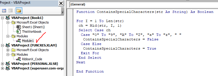
So open Excel. Press ALT+F11 to open VBE. Insert a module from the Insert menu. Copy the code below and paste it into the module.

Function ContainsSpecialCharacters(str As String) As Boolean
For I = 1 To Len(str)
 ch = Mid(str, I, 1)
 Select Case ch
  Case "0" To "9", "A" To "Z", "a" To "z", " "
   ContainsSpecialCharacters = False
  Case Else
   ContainsSpecialCharacters = True
  Exit For
 End Select
Next
End Function

Now the function is ready to be used.
Go to the worksheet in the workbook that contains the strings that you want to check.

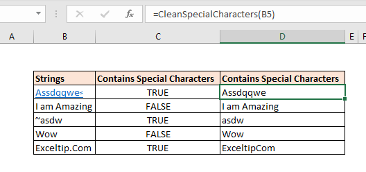
Write the below formula in cell C2:

=ContainsSpecialCharacters(B13)

It returns TRUE for the first string since it contains a special character. When you copy the formula down it shows FALSE for B14 string and so on. 

But strangely it shows TRUE for the last string «Exceltip.com». It is because it contains a dot (.). But why so? Let’s examine the code to understand.

How does the function work?

We are iterating through all the characters of the string using the For loop and mid function of VBA. The Mid function extracts one character at a time from string and stores it into ch variable.

For I = 1 To Len(str)
 ch = Mid(str, I, 1)

Now the main part comes. We use the select case statement to check what the ch variable contains.

We tell VBA to check if ch contains any of the defined values. I have defined 0 to 9, A to Z, a to z and » » (space). If c
h contains any of these, we set it’s value to False.

Select Case ch
  Case "0" To "9", "A" To "Z", "a" To "z", " "
   ContainsSpecialCharacters = False

You can see that we don’t have a dot (.) on the list and this is why we get TRUE for the string that contains dot. You can add any character to the list to be exempt from the formula.

If ch contains any character other than the listed characters, we set the function’s result to True and end the loop right there.

Case Else
   ContainsSpecialCharacters = True
Exit For

So yeah this how it works. But if you want to clean special characters, you will need to make some changes in the function.

How to Clean Special Characters From Strings in Excel?

To clean special characters from a string in Excel, I have created another custom function in VBA. The syntax of the function is:

=CleanSpecialCharacters(string)

This function returns a cleaned version of the string passed into it. The new string will not contain any of the special characters. 

The code of this function goes like this:

Function CleanSpecialCharacters(str As String)
  Dim nstr As String
  nstr = str
  For I = 1 To Len(str)
    ch = Mid(str, I, 1)
    Select Case ch
      Case "0" To "9", "A" To "Z", "a" To "z", " "
       'Do nothing
      Case Else
       nstr = Replace(nstr, ch, "")
    End Select
  Next
    CleanSpecialCharacters = nstr
End Function

Copy this in the same module you copied in the above code.

When you use this formula on the strings this is how the results will be:

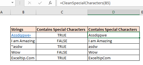
You can see every special character is removed from the string including the dot.

How does it work?

It works the same as the above function. The only difference is this function replaces every special character with a null character. Forms a new string and returns this string.

Select Case ch
      Case "0" To "9", "A" To "Z", "a" To "z", " "
       'ContainsSpecialCharacters = False
      Case Else
       nstr = Replace(nstr, ch, "")
     End Select

If you want to exempt any character from getting cleaned, you can add it to the list in the code. Excel will pardon that special character.

So yeah guys, this is how you can find and replace special characters from a string in Excel. I hope this was explanatory enough and helpful. If it doesn’t help you in solving your problem, let us know in the comments section below.

Related Articles:

How to Use TRIM function in Excel: The TRIM function is used to trim strings and clean any trailing or leading spaces from string. This helps us in the cleaning process of data a lot.

How to use the CLEAN function in Excel: Clean function is used to clean up unprintable characters from the string. This function is mostly used with the TRIM function to clean up imported foreign data.

Replace text from end of a string starting from variable position: To replace text from the end of the string, we use the REPLACE function. The REPLACE function uses the position of text in the string to replace it.

How to Check if a string contains one of many texts in Excel: To find check if a string contains any of multiple text, we use this formula. We use the SUM function to sum up all the matches and then perform a logic to check if the string contains any of the multiple strings.

Count Cells that contain specific text: A simple COUNTIF function will do the magic. To count the number of multiple cells that contain a given string we use the wildcard operator with the COUNTIF function.

Excel REPLACE vs SUBSTITUTE function: The REPLACE and SUBSTITUTE functions are the most misunderstood functions. To find and replace a given text we use the SUBSTITUTE function. Where REPLACE is used to replace a number of characters in string…

Popular Articles:

50 Excel Shortcuts to Increase Your Productivity | Get faster at your task. These 50 shortcuts will make you work even faster on Excel.

How to use Excel VLOOKUP Function| This is one of the most used and popular functions of excel that is used to lookup value from different ranges and sheets. 

How to use the Excel COUNTIF Function| Count values with conditions using this amazing function. You don’t need to filter your data to count specific values. Countif function is essential to prepare your dashboard.

How to Use SUMIF Function in Excel | This is another dashboard essential function. This helps you sum up values on specific conditions.

Need to retrieve specific characters from a string in Excel? If so, in this guide, you’ll see how to use the Excel string functions to obtain your desired characters within a string.

Specifically, you’ll observe how to apply the following Excel string functions using practical examples:

Excel String Functions Used	Description of Operation
LEFT	Get characters from the left side of a string
RIGHT	Get characters from the right side of a string
MID	Get characters from the middle of a string
LEFT, FIND	Get all characters before a symbol
LEFT, FIND	Get all characters before a space
RIGHT, LEN, FIND	Get all characters after a symbol
MID, FIND	Get all characters between two symbols

Excel String Functions: LEFT, RIGHT, MID, LEN and FIND

To start, let’s say that you stored different strings in Excel. These strings may contain a mixture of:

• Letters
• Digits
• Symbols (such as a dash symbol “-“)
• Spaces

Now, let’s suppose that your goal is to isolate/retrieve only the digits within those strings.

How would you then achieve this goal using the Excel string functions?

Let’s dive into few examples to see how you can accomplish this goal.

Retrieve a specific number of characters from the left side of a string

In the following example, you’ll see three strings. Each of those strings would contain a total of 9 characters:

• Five digits starting from the left side of the string
• One dash symbol (“-“)
• Three letters at the end of the string

As indicated before, the goal is to retrieve only the digits within the strings.

How would you do that in Excel?

Here are the steps:

(1) First, type/paste the table below into Excel, within the range of cells A1 to B4 (to keep things simple across all the examples to come, the tables to be typed/pasted into Excel, should be stored in the range of cells A1 to B4):

Identifier	Result
55555-End
77777-End
99999-End

Since the goal is to retrieve the first 5 digits from the left, you’ll need to use the LEFT formula, which has the following structure:

=LEFT(Cell where the string is located, Number of characters needed from the Left)

(2) Next, type the following formula in cell B2:

=LEFT(A2,5)

(3) Finally, drag the LEFT formula from cell B2 to B4 in order to get the results across your 3 records.

This is how your table would look like in Excel after applying the LEFT formula:

Identifier	Result
55555-End	55555
77777-End	77777
99999-End	99999

Retrieve a specific number of characters from the right side of a string

Wait a minute! what if your digits are located on the right-side of the string?

Let’s look at the opposite case, where you have your digits on the right-side of a string.

Here are the steps that you’ll need to follow in order to retrieve those digits:

(1) Type/paste the following table into cells A1 to B4:

Identifier	Result
ID-55555
ID-77777
ID-99999

Here, you’ll need to use the RIGHT formula that has the following structure:

=RIGHT(Cell where the string is located, Number of characters needed from the Right)

(2) Then, type the following formula in cell B2:

=RIGHT(A2,5)

(3) Finally, drag your RIGHT formula from cell B2 to B4.

This is how the table would look like after applying the RIGHT formula:

Identifier	Result
ID-55555	55555
ID-77777	77777
ID-99999	99999

Get a specific number of characters from the middle of a string

So far you have seen cases where the digits are located either on the left-side, or the right-side, of a string.

But what if the digits are located in the middle of the string, and you’d like to retrieve only those digits?

Here are the steps that you can apply:

(1) Type/paste the following table into cells A1 to B4:

Identifier	Result
ID-55555-End
ID-77777-End
ID-99999-End

Here, you’ll need to use the MID formula with the following structure:

=MID(Cell of string, Start position of first character needed, Number of characters needed)

(2) Now type the following formula in cell B2:

=MID(A2,4,5)

(3) Finally, drag the MID formula from cell B2 to B4.

This is how the table would look like:

Identifier	Result
ID-55555-End	55555
ID-77777-End	77777
ID-99999-End	99999

In the subsequent sections, you’ll see how to retrieve your desired characters from strings of varying lengths.

Gel all characters before a symbol (for a varying-length string)

Ready to get more fancy?

Let’s say that you have your desired digits on the left side of a string, BUT the number of digits on the left side of the string keeps changing.

In the following example, you’ll see how to retrieve all the desired digits before a symbol (e.g., the dash symbol “-“) for a varying-length string.

For that, you’ll need to use the FIND function to find your symbol.

Here is the structure of the FIND function:

=FIND(the symbol in quotations that you'd like to find, the cell of the string)

Now let’s look at the steps to get all of your characters before the dash symbol:

(1) First, type/paste the following table into cells A1 to B4:

Identifier	Result
111-IDAA
2222222-IDB
33-IDCCC

(2) Then, type the following formula in cell B2:

=LEFT(A2,FIND("-",A2)-1)

Note that the “-1” at the end of the formula simply drops the dash symbol from your results (as we are only interested to keep the digits on the left without the dash symbol).

(3) As before, drag your formula from cell B2 to B4. Here are the results:

Identifier	Result
111-IDAA	111
2222222-IDB	2222222
33-IDCCC	33

While you used the dash symbol in the above example, the above formula would also work for other symbols, such as $, % and so on.

Gel all characters before space (for a varying-length string )

But what if you have a space (rather than a symbol), and you only want to get all the characters before that space?

That would require a small modification to the formula you saw in the last section.

Specifically, instead of putting the dash symbol in the FIND function, simply leave an empty space within the quotations:

FIND(" ",A2)

Let’s look at the full steps:

(1) To start, type/paste the following table into cells A1 to B4:

Identifier	Result
111 IDAA
2222222 IDB
33 IDCCC

(2) Then, type the following formula in cell B2:

=LEFT(A2,FIND(" ",A2)-1)

(3) Finally, drag the formula from cell B2 to B4:

Identifier	Result
111 IDAA	111
2222222 IDB	2222222
33 IDCCC	33

Obtain all characters after a symbol (for a varying-length string )

There may be cases where you may need to get all of your desired characters after a symbol (for a varying-length string).

To do that, you may use the LEN function, which can provide you the total number of characters within a string. Here is the structure of the LEN function:

=LEN(Cell where the string is located)

Let’s now review the steps to get all the digits, after the symbol of “-“, for varying-length strings:

(1) First, type/paste the following table into cells A1 to B4:

Identifier	Result
IDAA-111
IDB-2222222
IDCCC-33

(2) Secondly, type the following formula in cell B2:

=RIGHT(A2,LEN(A2)-FIND("-",A2))

(3) Finally, drag your formula from cell B2 to B4:

Identifier	Result
IDAA-111	111
IDB-2222222	2222222
IDCCC-33	33

Obtain all characters between two symbols (for a varying-length string)

Last, but not least, is a scenario where you may need to get all of your desired characters between two symbols (for a varying-length string).

In order to accomplish this task, you can apply a mix of some of the concepts we already covered earlier.

Let’s now look at the steps to retrieve only the digits between the two symbols of dash “-“:

(1) First, type/paste the following table into cells A1 to B4:

Identifier	Result
IDAA-111-AA
IDB-2222222-B
IDCCC-33-CCC

(2) Then, type the following formula in cell B2:

=MID(A2,FIND("-",A2)+1,FIND("-",A2,FIND("-",A2)+1)-FIND("-",A2)-1)

(3) And finally, drag your formula from cell B2 to B4:

Identifier	Result
IDAA-111-AA	111
IDB-2222222-B	2222222
IDCCC-33-CCC	33

Excel String Functions – Summary

Excel string functions can be used to retrieve specific characters within a string.

You just saw how to apply Excel string functions across multiple scenarios. You can use any of the concepts above, or a mixture of the techniques described, in order to get your desired characters within a string.

Sometimes when we import data into Excel from an external data source such as a text file, it comes with special characters such as @, #, !,:, {}, &, ©, €, α, β, and so on. Before we can clean the data, we need to first find the characters and identify the cells that contain them.

In this tutorial, we will explore 3 methods that we can use to find special characters in Excel.

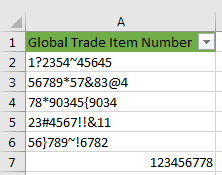
Example

We will use the following dataset that contains special characters to explain each of the methods:

Method 1: Use a User Defined Function (UDF)

Excel does not have an in-built Function to identify strings that have special characters. We can however create a User Defined Function to do the task.

We will create a UDF for this purpose by using the following steps:

1. Select cell B1 and type in “Has Special Characters”. This is the header row column B which will display the results of the UDF we create.
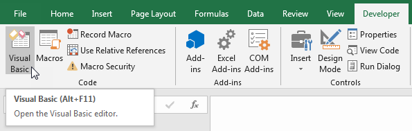
2. In the active worksheet press Alt + F11 to open the Visual Basic Editor. Alternatively, click Developer >> Code >> Visual Basic.

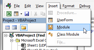
1. In the Project Window, right-click the ThisWorkbook object and click Insert >> Module on the shortcut menu.

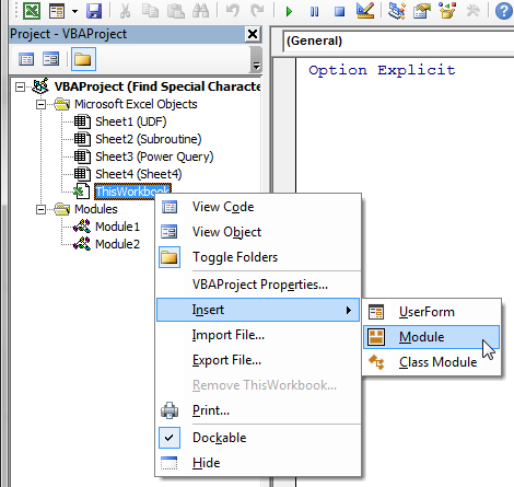
Alternatively, click Insert >> Module on the menu bar.

1. Type the following function procedure in the module.

Public Function IsSpecial(tString As String) As String     Dim L As Long     Dim tCh As String     IsSpecial = False     For L = 1 To Len(tString)         tCh = Mid(tString, L, 1)         If tCh Like «[0-9a-zA-Z]» Or tCh = «_» Then         Else             IsSpecial = True             Exit Function         End If     Next L End Function

1. Save the procedure and save the workbook as a macro-enabled workbook.
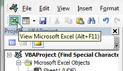
2. Press Alt + F11 to switch back to the active worksheet. Alternatively, click the View Microsoft Excel button on the toolbar.

1. Select cell B2 and type in the formula =IsSpecial(A2) as follows:

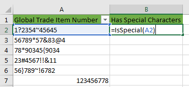
1. Press Enter and double-click or drag down the fill handle to copy the formula down the column.

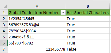
The function returns True for every cell that has special characters and False for every cell that does not have special characters.

Explanation of the User-Defined Function

• The IsSpecial Function is Public. This signifies that it can be accessed by all other procedures in all modules in the project.
• The function returns a value of the String data type.
• The function takes one argument of String data type.
• A Long variable and String variable are declared.
• The IsSpecial variable which also doubles up as the Function name is initialized to a False value.
• The For Next Loop construct checks each character of the text string that is passed to the Function against the identified non-special characters. If it looks like one of the non-special characters, the Function returns False meaning it is not a special character. If it does not look like any of the identified non-special characters, the Function returns True meaning it is a special character.

Method 2: Use Excel VBA Subroutine

In this method we use the following steps:

1. From the active worksheet that contains the data, we open Visual Basic Editor and insert a new module as explained in Method 1.
2. In the new module, we type the following Subroutine:

1 2 3 4 5 6 7 8 9 10 11 12 13 14 15 16 17 18 19 20 21 22 23

Sub paintCells() Dim tStrOK As String, tStr As String Dim rng As Range, rngCell As Range Dim j As Long tStrOK = «abcdefghijklmnopqrstuvwxyzABCDEFGHIJKLMNOPQRSTUVWXYZ0123456789,-.:;{}[]_» Set rng = Worksheets(«Subroutine»).UsedRange.SpecialCells(xlCellTypeConstants, xlTextValues) ‘   loop through all the cells with text constant values and ‘   paints in yellow the ones with characters not in tStrOK For Each rngCell In rng    tStr = rngCell.Value     For j = 1 To Len(tStr)         If InStr(tStrOK, Mid(tStr, j, 1)) = 0 Then             rngCell.Interior.Color = vbYellow             Exit For         End If     Next j Next rngCell End Sub

1. Save the Subroutine and save the workbook as a macro-enabled workbook.
2. Place the cursor anywhere in the Subroutine and press F5 to run the procedure.
3. Press Alt + F11 or click the View Microsoft Excel button on the toolbar to switch back to the active worksheet.

All the cells that contain special characters have a yellow background color.

Explanation of the Subroutine

• Five variables are declared.
• The specified nonspecial characters are assigned to the tStrOK variable.
• Our dataset is assigned to the rng variable using the Set keyword.
• The For Each Next construct checks each character of the values in the dataset to find out if it matches any character in the specified nonspecial characters. If it doesn’t match, it means it is a special character and the cell in which the character is contained is painted yellow.

Method 3: Use Power Query

We can use Power Query to find special characters in Excel.

We use the following steps:

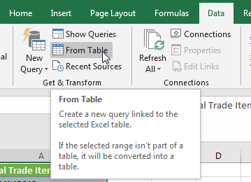
1. Select the dataset.
2. Click Data >> Get & Transform >> From Table.

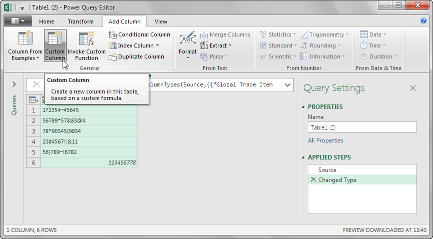
1. In Power Query Editor click Add Column >> General >> Custom Column.

1. In the Custom Column dialog box type in Special Characters in the New Column name box. Type the formula Text.Remove([Global Trade Item Number],{“A”..”z”,”0″..”9″}) in the Custom column formula box and click OK.

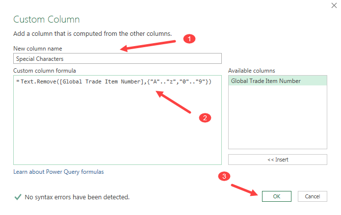
1. After the new column is inserted click Home >> Close >> Close & Load.

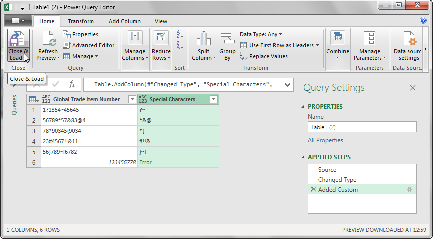
A new table is inserted in a different worksheet.

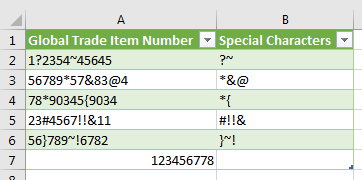
1. Click the down arrow in the header of column B and deselect the Blanks checkbox to hide the rows that have no special characters and click OK.

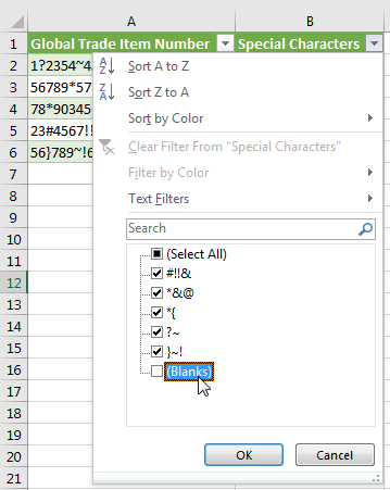
Only the cells with special characters are visible.

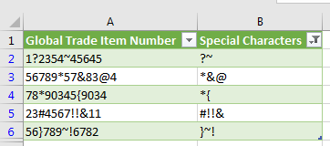
Explanation of the formula

=Text.Remove([Global Trade Item Number],{«A»..«z»,«0»..«9»})

• The Text.Remove function removes all occurrences of nonspecial characters from the dataset so that only the special characters remain.

Conclusion

When we import data into Excel from external sources such as text files, they may come with special characters such as @, #, !:. These characters make it difficult to analyze the data.

Finding the special characters is one step in the process of removing them.

In this tutorial we have looked at 3 methods we can use to find special characters in Excel. They are using a User Defined Function, applying Excel VBA Subroutine, and using Power Query.

Post Views: 2,312