Find averages on excel

This article describes the formula syntax and usage of the AVERAGE  function in Microsoft Excel.

Description

Returns the average (arithmetic mean) of the arguments. For example, if the range A1:A20 contains numbers, the formula =AVERAGE(A1:A20) returns the average of those numbers.

Syntax

AVERAGE(number1, [number2], …)

The AVERAGE function syntax has the following arguments:

• Number1    Required. The first number, cell reference, or range for which you want the average.

• Number2, …    Optional. Additional numbers, cell references or ranges for which you want the average, up to a maximum of 255.

Remarks

• Arguments can either be numbers or names, ranges, or cell references that contain numbers.

• Logical values and text representations of numbers that you type directly into the list of arguments are not counted.

• If a range or cell reference argument contains text, logical values, or empty cells, those values are ignored; however, cells with the value zero are included.

• Arguments that are error values or text that cannot be translated into numbers cause errors.

• If you want to include logical values and text representations of numbers in a reference as part of the calculation, use the AVERAGEA function.

• If you want to calculate the average of only the values that meet certain criteria, use the AVERAGEIF function or the AVERAGEIFS function.

Note: The AVERAGE function measures central tendency, which is the location of the center of a group of numbers in a statistical distribution. The three most common measures of central tendency are:

• Average, which is the arithmetic mean, and is calculated by adding a group of numbers and then dividing by the count of those numbers. For example, the average of 2, 3, 3, 5, 7, and 10 is 30 divided by 6, which is 5.

• Median, which is the middle number of a group of numbers; that is, half the numbers have values that are greater than the median, and half the numbers have values that are less than the median. For example, the median of 2, 3, 3, 5, 7, and 10 is 4.

• Mode, which is the most frequently occurring number in a group of numbers. For example, the mode of 2, 3, 3, 5, 7, and 10 is 3.

For a symmetrical distribution of a group of numbers, these three measures of central tendency are all the same. For a skewed distribution of a group of numbers, they can be different.

Tip: When you average cells, keep in mind the difference between empty cells and those containing the value zero, especially if you have cleared the Show a zero in cells that have a zero value check box in the Excel Options dialog box in the Excel desktop application. When this option is selected, empty cells are not counted, but zero values are.

To locate the Show a zero in cells that have a zero value check box:

• On the File tab, click Options, and then, in the Advanced category, look under Display options for this worksheet.

Example

Copy the example data in the following table, and paste it in cell A1 of a new Excel worksheet. For formulas to show results, select them, press F2, and then press Enter. If you need to, you can adjust the column widths to see all the data.

Data
10	15	32
7
9
27
2
Formula	Description	Result
=AVERAGE(A2:A6)	Average of the numbers in cells A2 through A6.	11
=AVERAGE(A2:A6, 5)	Average of the numbers in cells A2 through A6 and the number 5.	10
=AVERAGE(A2:C2)	Average of the numbers in cells A2 through C2.	19

---

How to calculate averages in Excel

Believe it or not, there are many different kinds of averages, and different ways to go about calculating them. The following methods are covered in this resource:

• AVERAGE
• AVERAGEA
• AVERAGEIF
• MEDIAN
• MODE
• Bonus: Nesting AVERAGE, LARGE and SMALL functions

AVERAGE

The most universally accepted average is the arithmetic mean, and Excel uses the AVERAGE function to find it. The Excel AVERAGE function is used to generate a number that represents a typical value from a range, distribution, or list of numbers. It is calculated by adding all the numbers in the list, then dividing the total by the number of values within the list. 

---

---

Syntax

The AVERAGE function in Excel is straightforward. The syntax is:

=AVERAGE(number1, [number2],...)

Ranges or cell references may be used instead of explicit values.

The AVERAGE function can handle up to 255 arguments, each of which may be a value, cell reference, or range. Only one argument is required, but of course, if you’re using the AVERAGE function, it’s likely you have at least two. 

The formula below will calculate the average of the numbers 100, 95, and 80.

=AVERAGE(100,95,80)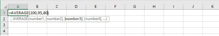

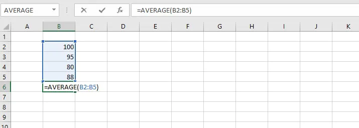
To calculate the average of values in cells B2, B3, B4, and B5 enter:

=AVERAGE(B2:B5)

This can be typed directly into the cell or formula bar, or selected on the worksheet by selecting the first cell in the range, and dragging the mouse to the last cell in the range. 

In order to calculate the average of non-contiguous (non-adjacent) cells, simply hold the Control key (or Command key — Mac users) while making the selections. 

If typing the cell references directly into the cell or formula bar, non-contiguous references are separated by commas. For example: 

=AVERAGE(B2:B5,B8)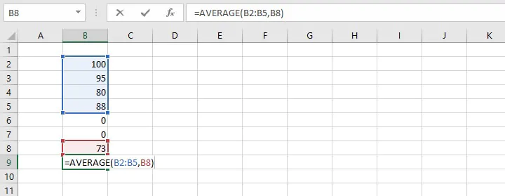

Remarks

When using the AVERAGE function, bear the following in mind.

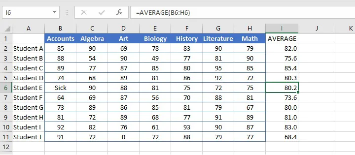
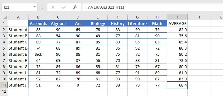
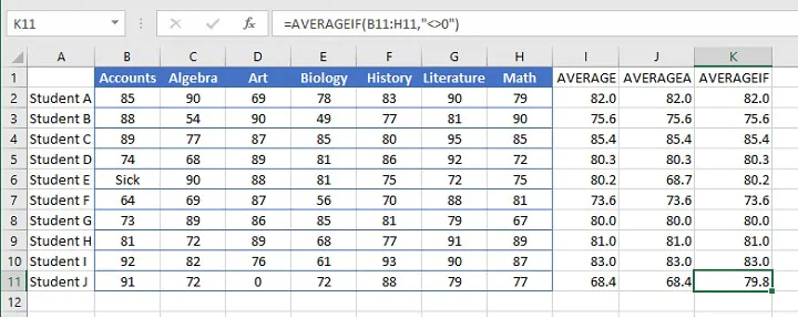
• Text values and empty cells are ignored.

The word “Sick” in cell B6 (below) causes the AVERAGE function to ignore that cell altogether. This means that the average score in cell I6 was computed using the values in the range C8 to H8, and the total was divided by 6 subjects instead of 7. 

• Zero values are included. 

When determining the number of values to divide the total by, zeros are considered valid amounts and will therefore reduce the overall average of the distribution. Notice that Student J’s average is quite different from Student E’s average, even though their grade totals were similar.

AVERAGEA

In order to eliminate this discrepancy, the AVERAGEA function may be used to include all values within a distribution, including text. The format is similar:

=AVERAGEA(value1, [value2],...)

A range or cell references may be used instead of explicit values.

AVERAGEA evaluates text values as zero, while the logical value TRUE is evaluated as 1. The logical value FALSE is considered a zero. 

Compare the difference in results between using AVERAGE and AVERAGEA in the example below.

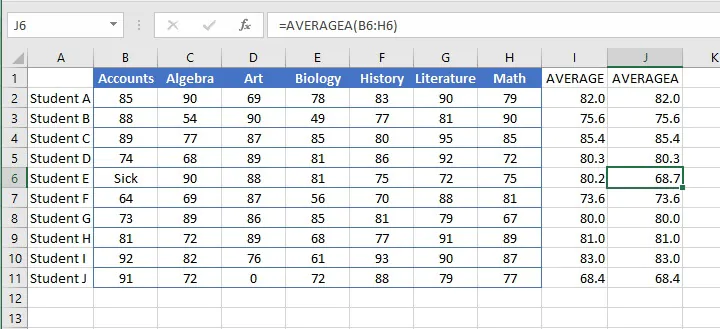The averages for Student E and Student J are now similar when using the AVERAGEA function.

---

Check out the Microsoft Excel Basic & Advanced course

---

AVERAGEIF

There are ways to find the average of only the numbers that satisfy certain criteria. With the AVERAGEIF function, Excel looks within the specified range for a stated condition, and then finds the arithmetic mean of the cells that meet that condition.

The syntax of the AVERAGEIF function is:

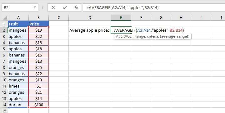
=AVERAGEIF(range,criteria,[average_range])

• The range is the location where we can expect to find cells that meet the criteria.
• The criteria are the value or expression that Excel should look for within the range.
• Average_range is an optional argument. This is the range of cells where the values to be averaged are located. If the average_range is omitted, the range is used.

AVERAGEIF example 1 

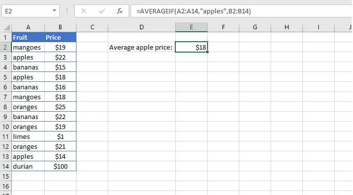
For example, from this list of various fruit prices, we can ask Excel to extract only the cells that say “apples” in column A, and find their average price from column B.

AVERAGEIF example 2

The criteria in an AVERAGEIF function may also be in the form of a logical expression, as in the example below:

=AVERAGEIF(B4:H4,"<>0")

The above formula will find the average of the values in the range B4 to H4 that are not equal to zero. Note that the third (optional) argument is omitted, therefore the cells in the range are used to calculate the average.

Since cells that are evaluated as zeros are omitted due to our criteria, notice the difference in Student E and J’s results below when using the AVERAGEIF function. 

In order to find the average of cells that satisfy multiple criteria, use the AVERAGEIFS function.

The arithmetic mean may be the most commonly-used method of finding the average, but it is by no means the only one. One outcome of using the arithmetic mean is that it allows very high or very low numbers to sway the outcome, thereby significantly altering the results. 

Take for example, the following list of numbers:

22, 1, 14, 21, 15, 16, 18, 100, 19, 19, 22, 25, 18

Finding the arithmetic mean would give a result of 23.8.

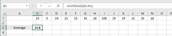However, looking closely at the distribution of the numbers on the list, we would hardly say that 23.8 is the average value of those numbers. The problem, of course, is that the number 100 is an outlier and increased the sum of the numbers. 

Therefore, in some situations, it is more desirable to use the MEDIAN function. This function determines the numerical order of the values being evaluated and uses the one in the middle as the average. 

The syntax is:

=MEDIAN(number1, [number2], …)

A range or cell references may be used instead of explicit values.

In the above example, the numerical order would be: 

1, 14, 15, 16, 18, 18, 19, 19, 21, 22, 22, 25, 100

There are 13 numbers in the distribution, making the seventh number the middle value. Therefore, the median would be 19.

If the number of values is an even number, the median would be determined by finding the average of the two numbers in the middle of the distribution. So, for the values 7,9,9,11,14,15 the median would be (9+11)/2=10.

The MEDIAN function ignores cells that contain text, logical values, or no value.

MODE

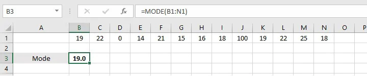
A third method for determining the average of a set of numbers is finding the mode, or the number that is repeated most often. 

There are currently three “mode” functions within Excel. The classic, MODE, follows the syntax of:

=MODE(number1, [number2],...)

In this function, Excel evaluates the values within the list or range, and selects the most frequently occurring number as the average value of the group.

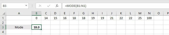
However, there are occasions when more than one number could be considered the mode. For example, consider the following list:

1, 14, 15, 16, 18, 18, 19, 19, 21, 22, 22, 25, 100

The numbers 18, 19, and 22 each appear two times. Which one is the mode? Microsoft chooses the first-appearing value as the mode — in the above case, 18.

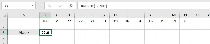
If these same numbers were arranged in the reverse order, then 22 would be considered the mode. 

If the numbers were arranged in a random order, then Excel would select from 18, 19, and 22 based on whichever number appeared in the distribution first.

For example, in the list: 

19, 22, 1, 14, 21, 15, 16, 18, 100, 19, 22, 25, 18

The MODE function considers 19 as the mode.

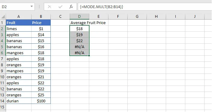
MODE.MULT

The MODE.MULT function is a solution to the discrepancies experienced in the above scenario. It allows us to anticipate and account for the possibility that there may be more than one mode within a group of numbers. 

The syntax is:

=MODE.MULT(number1, [number2],...)

Since MODE.MULT is an array (CSE) function, these are the steps when using this function:

1. Select a vertical range for the output 
2. Enter the MODE.MULT formula
3. Simultaneously select Control + Shift + Enter 

Pressing Control + Shift + Enter (CSE) together will cause Excel to automatically place braces (curly brackets) around the formula, and will return a “spill” of results equal to the number of cells selected in Step 1. If there is more than one mode, they will be displayed vertically in the output cells. The MODE.MULT function will return the “#N/A” error if:

• there are no duplicate values, or
• there are no additional modes in the output range. 

MODE.SNGL

Like the MODE.MULT function, the MODE.SNGL function was rolled out with Excel 2010. The syntax is:

=MODE.SNGL(number1, [number2],...]

The MODE.SNGL function behaves like the classic MODE function in determining the output.

Creative uses of the AVERAGE function

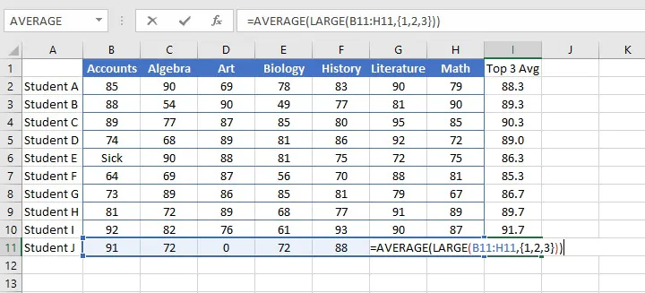
Top 3

We can combine the AVERAGE function with the LARGE function to determine the average of the top “n” number of values. 

The LARGE function extracts the n^th  largest number from a range, using the format

=LARGE(array, k)

where k is the n^th number.

Using this format, we can display a number in the 1st, 2nd, 5th, or any rank. 

In order to get the average of the three largest numbers in a range, we would nest the AVERAGE and LARGE functions as follows:

=AVERAGE(LARGE(array, {1,2,3}))

When we type braces around the k argument, Excel identifies the first, second, and third largest numbers in the array, and the AVERAGE function finds their average.

Bottom 3

We can use a similar logic to find the bottom 3 of a group of numbers using the SMALL function.

The following format will find the average of the three smallest numbers in the array.

=AVERAGE(SMALL(array, {1,2,3}))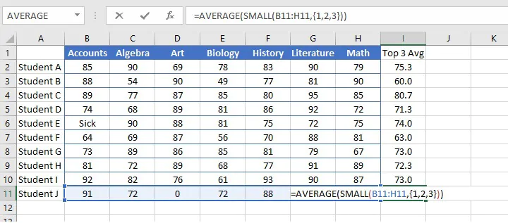

The three main methods of finding the average within Excel are the AVERAGE (mean), MEDIAN (middle), and MODE (frequency) functions. They are all easy to use, so choose the one that’s right for your type of data and the questions you want to answer.

Learn more Excel formulas and functions

To learn more useful formulas, functions, and real-world Excel skills, try the GoSkills Basic and Advanced Excel course today. 

В процессе различных расчетов и работы с данными довольно часто требуется подсчитать их среднее значение. Оно рассчитывается путем сложения чисел и деления общей суммы на их количество. Давайте выясним, как вычислить среднее значение набора чисел при помощи программы Microsoft Excel различными способами.

Стандартный способ вычисления

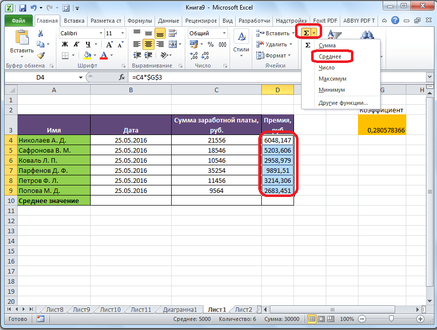
Самый простой и известный способ найти среднее арифметическое набора чисел — это воспользоваться специальной кнопкой на ленте Microsoft Excel. Выделяем диапазон чисел, расположенных в столбце или в строке документа. Находясь во вкладке «Главная», жмем на кнопку «Автосумма», которая расположена на ленте в блоке инструментов «Редактирование». Из выпадающее списка выбираем пункт «Среднее».

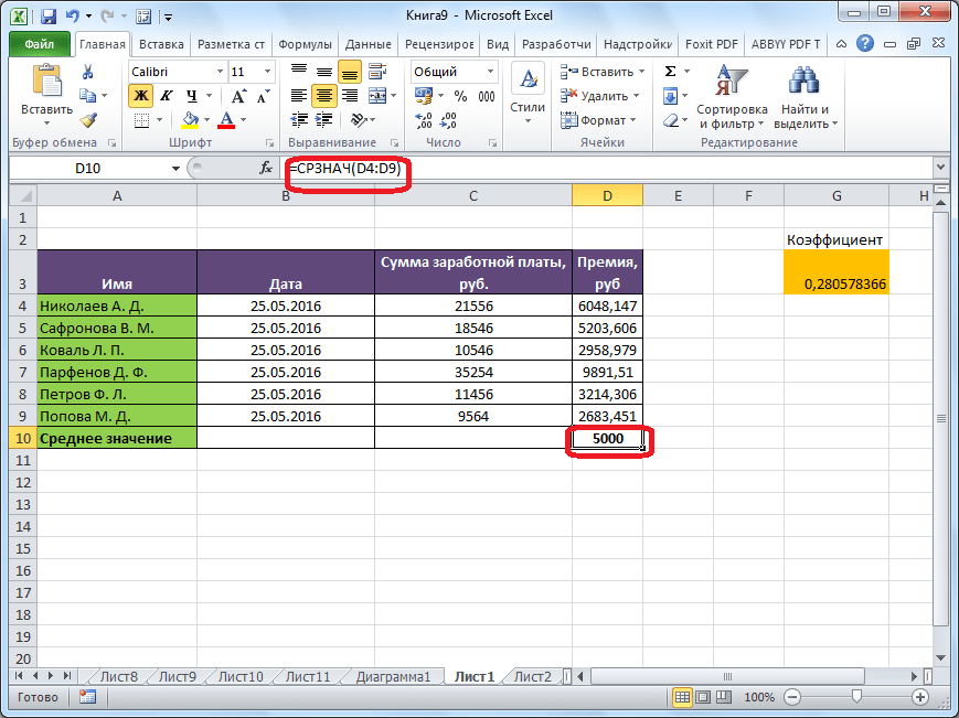
После этого, с помощью функции «СРЗНАЧ», производится расчет. В ячейку под выделенным столбцом, или справа от выделенной строки, выводится средняя арифметическая данного набора чисел.

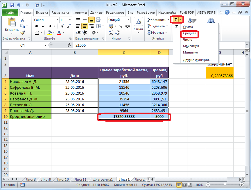
Этот способ хорош простотой и удобством. Но, у него имеются и существенные недостатки. С помощью этого способа можно произвести подсчет среднего значения только тех чисел, которые располагаются в ряд в одном столбце, или в одной строке. А вот, с массивом ячеек, или с разрозненными ячейками на листе, с помощью этого способа работать нельзя.

Например, если выделить два столбца, и вышеописанным способом вычислить среднее арифметическое, то ответ будет дан для каждого столбца в отдельности, а не для всего массива ячеек.

Вычисление с помощью Мастера функций

Для случаев, когда нужно подсчитать среднюю арифметическую массива ячеек, или разрозненных ячеек, можно использовать Мастер функций. Он применяет все ту же функцию «СРЗНАЧ», известную нам по первому методу вычисления, но делает это несколько другим способом.

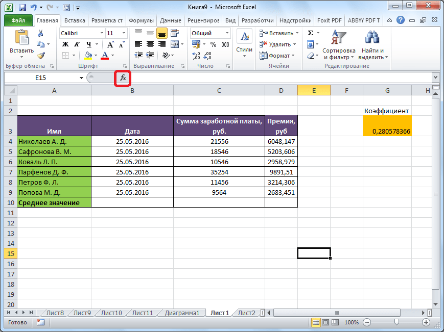
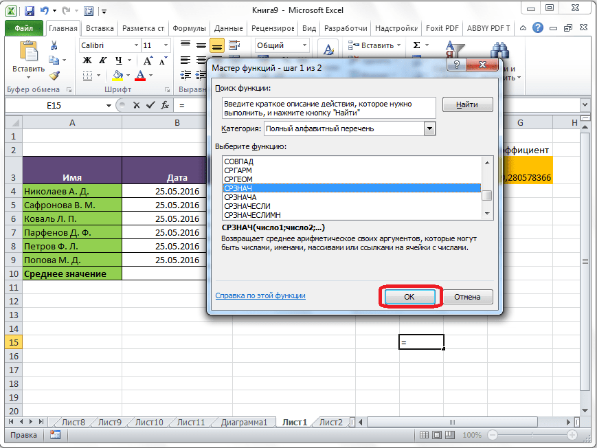
Кликаем по ячейке, где хотим, чтобы выводился результат подсчета среднего значения. Жмем на кнопку «Вставить функцию», которая размещена слева от строки формул. Либо же, набираем на клавиатуре комбинацию Shift+F3.

Запускается Мастер функций. В списке представленных функций ищем «СРЗНАЧ». Выделяем его, и жмем на кнопку «OK».

Открывается окно аргументов данной функции. В поля «Число» вводятся аргументы функции. Это могут быть как обычные числа, так и адреса ячеек, где эти числа расположены. Если вам неудобно вводить адреса ячеек вручную, то следует нажать на кнопку расположенную справа от поля ввода данных.

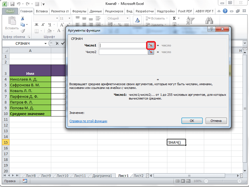
После этого, окно аргументов функции свернется, а вы сможете выделить ту группу ячеек на листе, которую берете для расчета. Затем, опять нажимаете на кнопку слева от поля ввода данных, чтобы вернуться в окно аргументов функции.

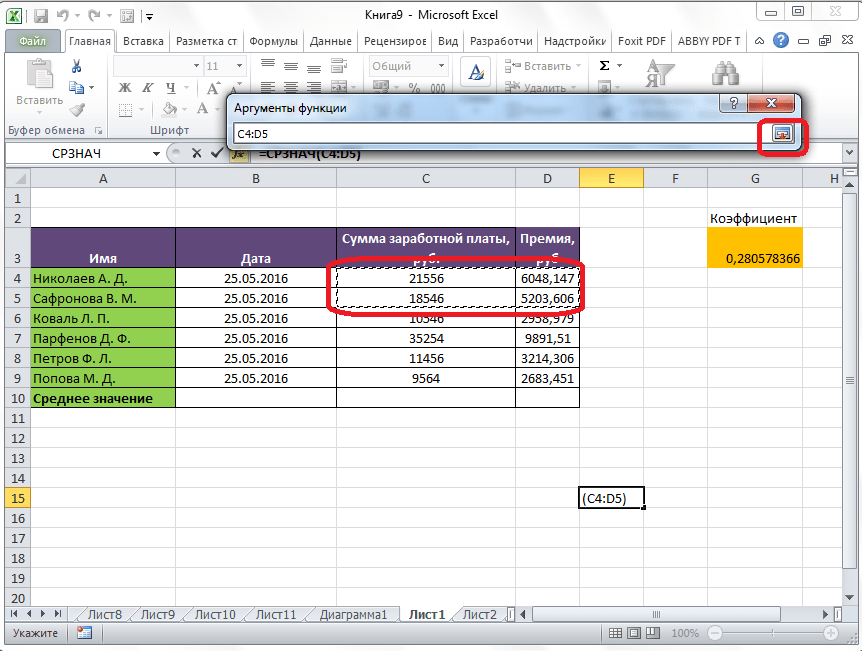
Если вы хотите подсчитать среднее арифметическое между числами, находящимися в разрозненных группах ячеек, то те же самые действия, о которых говорилось выше, проделывайте в поле «Число 2». И так до тех пор, пока все нужные группы ячеек не будут выделены.

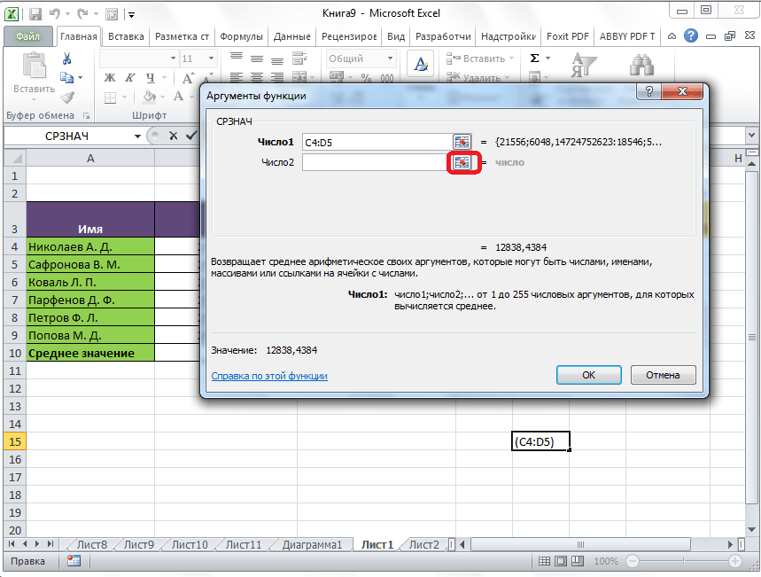
После этого, жмите на кнопку «OK».

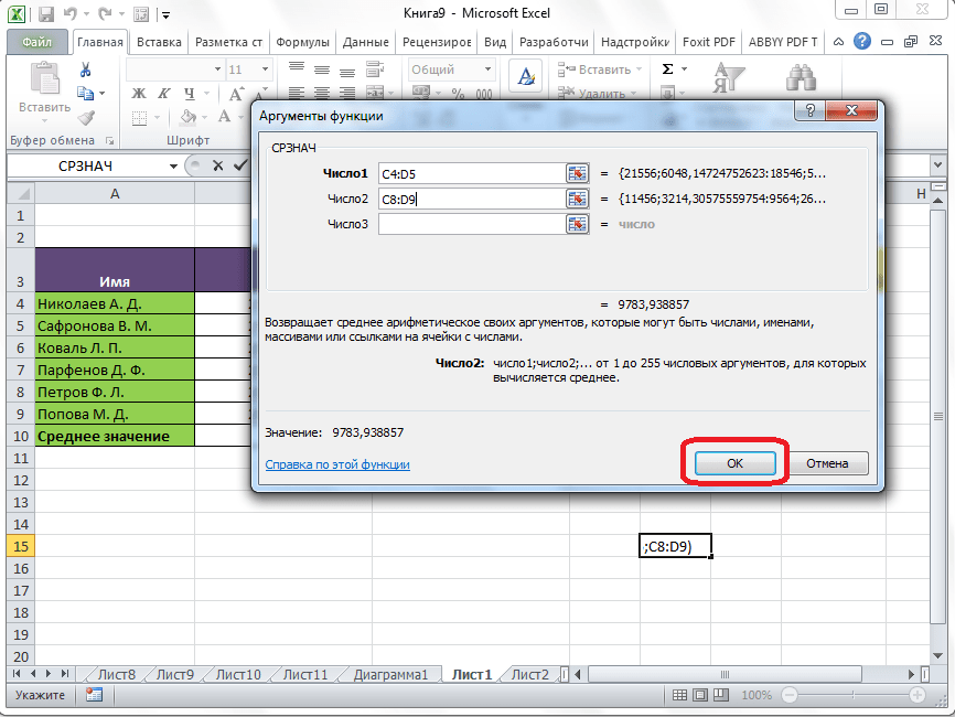
Результат расчета среднего арифметического будет выделен в ту ячейку, которую вы выделили перед запуском Мастера функций.

Панель формул

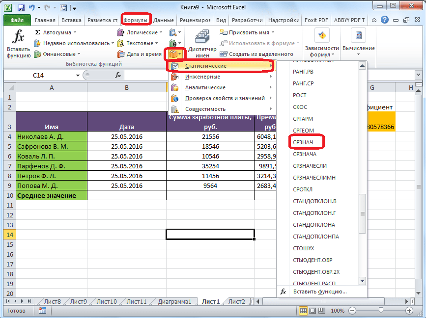
Существует ещё третий способ запустить функцию «СРЗНАЧ». Для этого, переходим во вкладку «Формулы». Выделяем ячейку, в которой будет выводиться результат. После этого, в группе инструментов «Библиотека функций» на ленте жмем на кнопку «Другие функции». Появляется список, в котором нужно последовательно перейти по пунктам «Статистические» и «СРЗНАЧ».

Затем, запускается точно такое же окно аргументов функции, как и при использовании Мастера функций, работу в котором мы подробно описали выше.

Дальнейшие действия точно такие же.

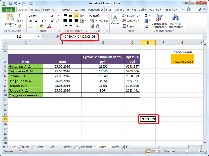
Ручной ввод функции

Но, не забывайте, что всегда при желании можно ввести функцию «СРЗНАЧ» вручную. Она будет иметь следующий шаблон: «=СРЗНАЧ(адрес_диапазона_ячеек(число); адрес_диапазона_ячеек(число)).

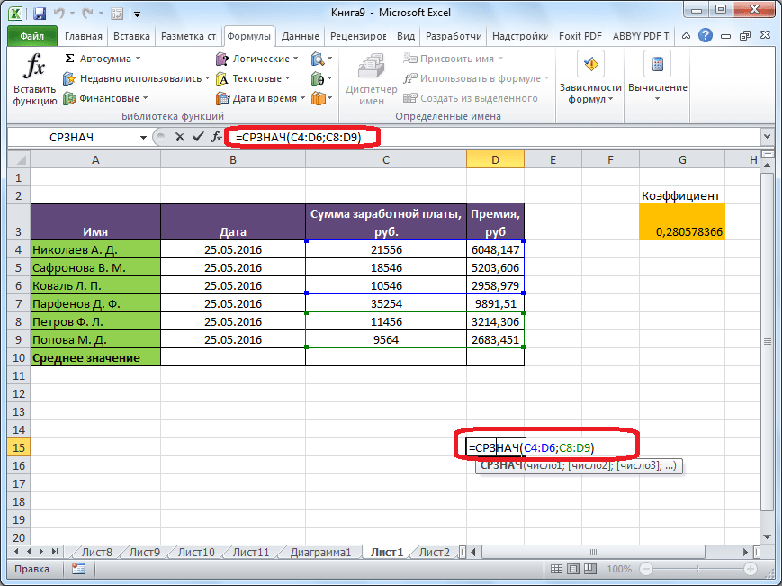
Конечно, этот способ не такой удобный, как предыдущие, и требует держать в голове пользователя определенные формулы, но он более гибкий.

Расчет среднего значения по условию

Кроме обычного расчета среднего значения, имеется возможность подсчета среднего значения по условию. В этом случае, в расчет будут браться только те числа из выбранного диапазона, которые соответствуют определенному условию. Например, если эти числа больше или меньше конкретно установленного значения.

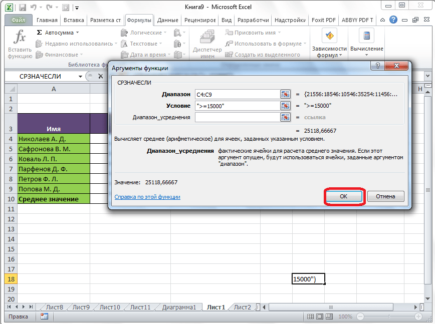
Для этих целей, используется функция «СРЗНАЧЕСЛИ». Как и функцию «СРЗНАЧ», запустить её можно через Мастер функций, из панели формул, или при помощи ручного ввода в ячейку. После того, как открылось окно аргументов функции, нужно ввести её параметры. В поле «Диапазон» вводим диапазон ячеек, значения которых будут участвовать в определении среднего арифметического числа. Делаем это тем же способом, как и с функцией «СРЗНАЧ».

А вот, в поле «Условие» мы должны указать конкретное значение, числа больше или меньше которого будут участвовать в расчете. Это можно сделать при помощи знаков сравнения. Например, мы взяли выражение «>=15000». То есть, для расчета будут браться только ячейки диапазона, в которых находятся числа большие или равные 15000. При необходимости, вместо конкретного числа, тут можно указать адрес ячейки, в которой расположено соответствующее число.

Поле «Диапазон усреднения» не обязательно для заполнения. Ввод в него данных является обязательным только при использовании ячеек с текстовым содержимым.

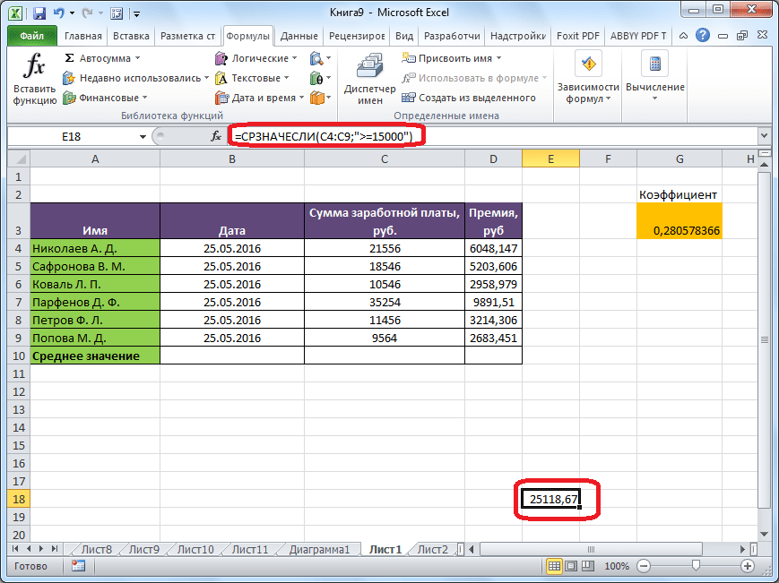
Когда все данные введены, жмем на кнопку «OK».

После этого, в предварительно выбранную ячейку выводится результат расчета среднего арифметического числа для выбранного диапазона, за исключением ячеек, данные которых не отвечают условиям.

Как видим, в программе Microsoft Excel существует целый ряд инструментов, с помощью которых можно рассчитать среднее значение выбранного ряда чисел. Более того, существует функция, которая автоматически отбирает числа из диапазона, не соответствующие заранее установленному пользователем критерию. Это делает вычисления в приложении Microsoft Excel ещё более удобными для пользователей.