
-
VBA Macros
-
Last updated on December 10, 2019

Chandoo
Filtering a list is a powerful & easy way to analyze data. But filtering requires a lot of clicks & typing. Wouldn’t it be cool if Excel can filter as you type, something like this:

Let’s figure out how to do this using some really simple VBA code.
Filter as you type – VBA tutorial
Step 1: Set up a list with values you want to filter.
To keep it simple, let’s assume your values are in an Excel table named States.

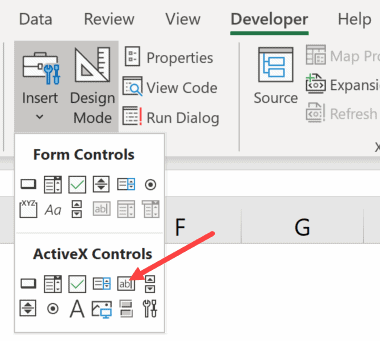
Step 2: Insert a text box active-x control
Go to developer tab and click on insert > text box (active-x) control.

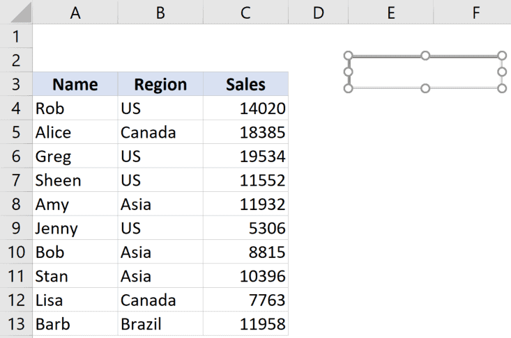
Insert this control on your spreadsheet, preferably above the states table.
[Related: Introduction to Excel form controls – article, podcast]
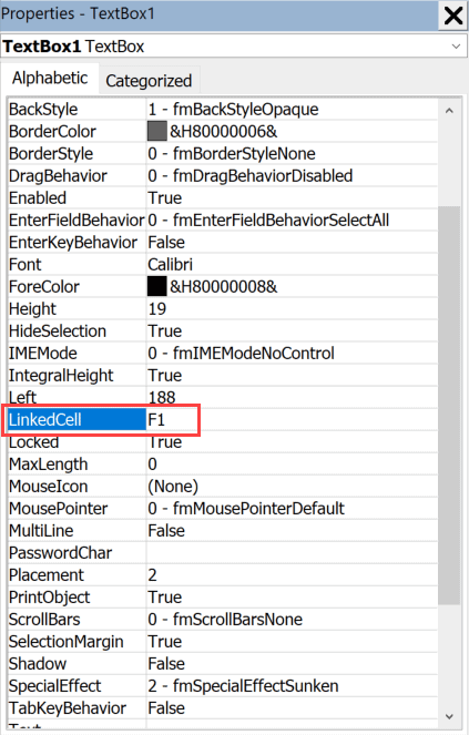
Step 3: Link text box to a blank cell.
Click on properties button in developer tab and set linked cell property of text box to an empty cell in your worksheet. I set mine to E4.

Step 4: Add CHANGE event to text box
Right click on the text box and choose “view code”. This will take you to Visual Basic Editor (VBE) and creates an emtpy textbox1_change() event.
Quick: What is an event?
Answer: An Event is a macro (VBA code) that runs when a certain condition is satisfied. For example, textbox1_change event runs whenever you change the textbox value (ie type something in to it, edit it or delete its contents).
We need to write VB code to filter our table (states), whenever user types something in to the text box. This code is just one line!
You can use below code or come up with your own version.
ActiveSheet.ListObjects("states").Range.AutoFilter Field:=1, Criteria1:="*" & [e4] & "*", Operator:=xlFilterValuesReplace the words states and e4 with your own table name & linked cell address.
That is all. Close VBE and return to Excel.
Step 5: Play with filter as you type macro
If you are in design mode, exit it by clicking on “design mode” button in developer tab.
Click on text box and type something. Your table gets filtered as you type, just like magic!
Want to filter multiple column table? Use this macro instead…
The above code works fine if you have just one column data. What if you need to filter a giant table with several columns? Our reader Chris thought about the problem and shared below approach.
- Create a new column at the end of your table that concatenates all column data. Something like this
=CONCAT(Table3[@[first col]:[last col]]&” “) - Now add Worksheet_Change event (or Textbox_change event) to monitor the input cell
- Apply filter on the concatenated column. Sample code below.
Private Sub Worksheet_Change(ByVal Target As Range)
    Dim KeyCells As Range
    Set KeyCells = Range("search_string")

    If Not Application.Intersect(KeyCells, Range(Target.Address)) _
           Is Nothing Then
            FastFilter (KeyCells.Value)
    End If
End Sub


Sub FastFilter(sch As String)

    Dim lo As ListObject
    Set lo = ActiveSheet.ListObjects(1)
    lastcol = lo.ListColumns.Count

    If lo.AutoFilter.FilterMode Then
        lo.AutoFilter.ShowAllData
        lo.Range.AutoFilter Field:=lastcol, Criteria1:= _
            Array("*" + sch + "*"), Operator:=xlFilterValues
        Else
        lo.Range.AutoFilter Field:=lastcol, Criteria1:= _
            Array("*" + sch + "*"), Operator:=xlFilterValues
        End If
    Range("search_string").Select
End Sub
Filter on any column – VBA Trick – Explanation video
Watch below video to understand how “filter on any column with VBA” trick works. You can watch it here or on my YouTube Channel.
Download filter as you type example macro
Please click here to download filter as you type example workbook. As a bonus, the download workbook as code to clear / reset filters too. Examine the code to learn more.
Click here to download the FastFilter code example file.
More awesome ways to filter your data
If you are often filtering your data, you will find below tips handy:
- Filter a table by combination of values quickly
- How to use advanced filters to extract values that meet multiple criteria in one go
- Using report filters in Excel pivot tables
- Slicers – filters for the new generation – how to use them?
- Filter odd or even rows only
Awesome as you learn:
There is no doubt that you will get awesome at your work by learning new & powerful ways to do it.
If you want to learn how to use VBA to automate your work, please consider our online VBA classes. This comprehensive program teaches VBA macros from scratch to advanced level thru step-by-step video tutorials.
Click here to know more about the VBA classes and enroll today.
Share this tip with your colleagues
-
94 Comments -
Ask a question or say something… -
Tagged under
awesome august, data filters, downloads, macros, no ads, no-nl, quick tip, screencasts, VBA, videos
-
Category:
VBA Macros

Welcome to Chandoo.org
Thank you so much for visiting. My aim is to make you awesome in Excel & Power BI. I do this by sharing videos, tips, examples and downloads on this website. There are more than 1,000 pages with all things Excel, Power BI, Dashboards & VBA here. Go ahead and spend few minutes to be AWESOME.
Read my story • FREE Excel tips book

Chandoo is an awesome teacher
5/5

From simple to complex, there is a formula for every occasion. Check out the list now.

Calendars, invoices, trackers and much more. All free, fun and fantastic.

Still on fence about Power BI? In this getting started guide, learn what is Power BI, how to get it and how to create your first report from scratch.

- Excel for beginners
- Advanced Excel Skills
- Excel Dashboards
- Complete guide to Pivot Tables
- Top 10 Excel Formulas
- Excel Shortcuts
- #Awesome Budget vs. Actual Chart
- 40+ VBA Examples
94 Responses to “Filter as you type [Quick VBA tutorial]”
-
 Rahul says:
 I am blank in Macros, tried copying the code. But got Run-time error:9. Please help and also suggest some resources to grab the basics of Macros (for beginners and intermediate).
-
Jitendra sharma says:
Dear Chandoo,
Please help me.
I want to know how many times visit in a company within a week & within a day.
DATE Visiter Name
01-Aug-15 JVS
01-Aug-15 FAZE
01-Aug-15 TREND
01-Aug-15 SHAHI
03-Aug-15 WAZIR
03-Aug-15 JVS
03-Aug-15 CELLO
03-Aug-15 HANUNG
03-Aug-15 WAZIR
04-Aug-15 TRIDENT
04-Aug-15 ANIKET
05-Aug-15 JVS
05-Aug-15 DESIGNCO
05-Aug-15 ABHITEX
05-Aug-15 JVS
05-Aug-15 CELLO
05-Aug-15 SHAHI
06-Aug-15 JEWEL
06-Aug-15 JEWEL
07-Aug-15 TREND
07-Aug-15 NAVNEET
07-Aug-15 KAPOOR
07-Aug-15 TREND
08-Aug-15 RAMESH
07-Aug-15 ALOK
07-Aug-15 NAVNEET
08-Aug-15 FAZE
08-Aug-15 SHAHI
08-Aug-15 LUXOR
08-Aug-15 WELSPUN
08-Aug-15 ABHII want to count.
It means «cello» visiter visit in office 2 times with 1st to 8th Aug-15.
Cello 2
-
Kuldeep Mishra says:
=SUMPRODUCT(—($A$2:$A$32<=J4)*($B$2:$B$32=»CELLO»))
-
Jitendra sharma says:
Dear Kuldeep,
I am not understand why u are using «J4» pls clarify the same.
Thanks
Jitendra-
Kuldeep Mishra says:
j4 is the cell reference you just need to put date instead CELL REFERENCE.
-
PRADEE PRAJAPATI says:
Hi Kuldeep,
I am getting this output «08-Aug-15», «-3″ when i use this formula- =SUMPRODUCT(-($I$3:$I$33<=I35)*($J$3:$J$33=»SHAHI»))
-
-
-
-
Hamid MilaniNia says:
Have you tried to utilize PowerQuery utilizing converting the range into a table then bring it in Power Query, Split the columns by selecting the first 9 characters from left, rename the columns to Dates, Name then bring the table back into Excel, Insert a Slicer select name as a filter. Simply click on the name and the table displays only days which the Visits where made.
-
Power by PK says:
Hi,
Jitendra JiSimple
If Date and Name (B2:B20) in separate column..Type a visitor name (D2) in outside of table and use formula
=countif(B2:B20,D2)Reply if formula work as your think.
-
-
Chris O’Neill says:
Chandoo,
This is a great tip. I modified it to search all columns in a data table and filter if any column shows the value. I was using conditional color coding but this is much nicer. Let me know if you want the sample sheet. — Chris
-
Hi Chris,
That is lovely. Please post the VBA code in comments or email me at chandoo.d@gmail.com. I would like to learn from it and share it with rest of the readers.
-
Chris O’Neill says:
I sent you the model — there is no VBA code. I use only your code for the filter as you type. I created a formula means to create a hidden column where it searches all the other columns. Brute force but works like a top. I also ended up bailing on the filter as you go when the database got too big. Now I just have a running total and click that box to filter once. Please let me know if you have any questions or concerns. Great site, nice people in your forum. happy to share what little I Know.
Chris
-
-
Chris says:
Chris,
I know this was a long time back, but would you happen to know the formula you used to search the entire table? This is something I’m trying to do, but to no avail right now.Thanks,
Chris-
Chris,
I detailed the formula above in an article. Let me know if you have any questions or concerns.
Chris O.
-
Chris says:
Maybe I’m just missing it, but can you please provide the article? Thanks in advance!
-Chris
-
-
-
Bala says:
Chris can you share the old sheet where you modified using the hidden column one.Can mail to balam1986@gmail.com
-
Bala,
I resent the link. If you just click my name you go to the share site. I would delete your email now that you know how to contact me. — Chris
-
-
-
slsuser says:
This is great but seems to only filter on the the starting characters in the strings.
Can the code be changed to a sequential search to show the results where the combinations entered appear anywhere within the string?
For example, using the original data, if I type in «or» then florida and georgia would display in the list.-
@Slsuer:
Can you double check? The filtering should work for occurrence anywhere.
-
-
slsuser says:
Thanks for your reply….
Apologies, it may be working.
Having issues with Excel right now and can only open older version. Will check next weekend upon arrival of new pc. -
Tim says:
Chandoo,
This is a great method. I have one question though.
Say I want to filter by column «region» in the «states» table how would I go about doing that? I tried replacing «states» with the column name «states[[#All],[Region]]» and «states[Region]», but to no avail.
Thank you!
Tim -
Lloyd says:
Awesome as always,
I was thinking about trying to us something along these lines to replace a slicer (for a very long list) in a pivot table. My initial thought were;ActiveSheet.PivotTables(«PivotTable1»).PivotFields(«Items»).Range.AutoFilter Field:=1, Criteria1:=»*» & [a1] & «*», Operator:=xlFilterValues
But this failed abysmally with a 438 error.
Any thoughts on if this is possible and the correct syntax to make it work?
Thanks again
Lloyd
-
Rick says:
Chandoo,
Excellent example. You state «To keep it simple, let’s assume your values are in an Excel table». Must the data be in an Excel table? I can’t seem to make it work otherwise.
-
kasawubu says:
Dear Chandoo,
this is a great tip.
Tried to use it in an example on my own (Excel 2013).
Replaced name and linked cell, but always get vba error 9 ‘Subscript out of range’.Tried different things already — no success.
How can I make it work? Thanks.-
John says:
Did you convert your data into a table? If you created a named range instead you will likely get Error 9.
-
kasawubu says:
Yes, I used a table, but got the error nevertheless.
-
kasawubumail says:
Got it: made a mistake by not using the correct table Name.
-
-
-
-
nikhil says:
Hey chandoo, could please explain this because I am getting run error 9 .
-
@Nikhil
Run Error 9 is usually because you have used a variable outside its defined range or have tried to use a variable which hasn’t been defined
eg: Setting an Integer variable to more than 32,767
or trying to use a variable which hasn’t been defined
eg: defining a workbook as a name and then referencing the work book when it isn’t openedCan you post the file or VBA Code in question and highlight where it is failing?
-
nikhil says:
@hui
Thanks for your reply and I understood my problem… I have one requirement. The requirement is that I want the same filter as you type but I want to filter as you type number is that possible?
-
-
-
slsuser says:
to Nikhil…
To me it appears that the numeric as not filtering because they are numeric. I entered a number as 65432 and with a leading ‘ (single quote) to cause the number to be entered as text and the filter works.
that would be a lot of effort.
I then formatted the table as text instead of general. New numeric entries added to the end of the table were treated as text and filtered properly.
I see the bets way would be to convert all entries to text in the VBA but I haven’t figured that out. Formatting the E4 value as chr fails on text. Perhaps need to inspect the value to see if numeric and then process differently if numeric?? not sure but this is food for thought.-
nikhil says:
@ slsuser
Thanks for your for reply
I already tried converting numeric to text by using both the methods as u mentioned but still the filter is not working????. Could please share the code wic u used it
Thanks in advance -
nikhil says:
@ slsuser
Thanks for your for reply
I already tried converting numeric to text by using both the methods as u mentioned but still the filter is not working????. Could please share the code wic u used it
Thanks in advance-
slsuser says:
Nikhil,
No coding is required. You must format the column as TEXT before inputting the values. The table in the example spreadsheet (filter-as-you-type.xlsm) is formatted as «General» so numbers are treated as numbers and alpha is treated as text which is why the filter fails on only numeric values.
Simply select your entire table and change the format to text. All NEW entries (at the bottom of the table) will be formatted as text.
Existing entries will NOT automatically change to text. If there are not to many you can go to each cell and press F2 and enter and the number should change to Text format.
I have tried this and it works without coding.
Note if you plan to perform any numeric functions you will need to convert back to number format in your formulas.-
nikhil says:
Slsuser,
Thanks for the tips its working
-
-
-
-
Hey, I liked the search but wanted to be able to have all columns searchable.
1.) I use data table.
2.) I created column that does a find of the string against each of the columns. (I hide that column normally)
3.) I use Chandoo’s code to set that search column to 1 which is the value given when any of the other columns find the string or any part of the string.I posted a sample doc to google here:
https://drive.google.com/folderview?id=0B3NPE3t4gC36WDMxWnpSS1EtbkE&usp=sharing
Hope this helps someone as much as the tip helped me.
Chris
-
nikhil says:
Hey thanks for sharing the file it’s quiet interesting.I just need to understand how that if nesting work as filter
-
Chris says:
N,
Okay — here is how the nesting works.
Find looks for the string inside a column
If it finds no string an error is thrown
I use iferror to trap the error and make a 1 if no error exists and zero if it does exist
Thus the string comes from the dialog box and creates a 1 for each column that contains the text in the dialog box
I add all the 1 ‘s together and then creat a formula that says if the total of the 1 ‘s. Is greater than zero put. 1 or true in the cell to the leftThen I use the filter aa you type but filter on 1 or true.
I hope this helps. I use this for over 600 paragraphs across 10 columns and it works well.. If a little slow….
Chris
-
-
Ron says:
Hi Chris,
I would be very happy if you could please post your sample doc to Google drive once again. I am looking for exactly what you are describing.
Thks.
-
Chris O’Neill says:
Hi Ron,
Per your request, I am reposting the link to the article and model I wrote.
https://drive.google.com/drive/folders/0B3NPE3t4gC36OWVBT2lsNzB0LWM?usp=sharing
Since then, I have moved on to different approaches to the problem as this solution starts to slow down as the database grows. If you are good with VBA I can share some functions and subroutines that filter tables quicker than this way. — Chris O
-
Ron says:
Chris,
First impression — very good. I dumped 60,000 records that have 23 columns (1.4 million cells). Yes, it currently only checks the first 5 columns, but it is very fast. No — Unfortunately, I am not good with VBA.
This does serve a purpose for me. However, what I am ideally looking for is something where I can have the ability to do multiple search & filtering by column across the board.
Can this be more or less easily modified to adapt to what I am looking for ?
Many thanks for the quick posting Chris. I took a chance that you would respond after your original post from a couple of year’s back.
Ron
-
You probably have a decent processor and ample memory. I am happy you get value from this.
You can modify it easily to check all the columns. Look at the formula in the first column… replace the text «column2» with the exact text of your first data column… then replace column5 with the exact name of your last column. I like to create a column on the end of my table called «LastColumn» then hide it which means the formula will always work if I use the same names.
=NOT(ISERROR(MATCH(«*»&IF(ISBLANK(search_string),RAND(),search_string)&»*»,TEXT(tb_main[@[Column2]:[Column5]],»0.00000″),0)))
-
I updated the file to reflect the changes. A few tips and tricks:
1.) Cope and paste the formula to notepad, clear the whole search column and paste it in the first cell which will create a clean uniform set of searches.
2.) Note that you will get a cell error warning if your last column is full of blank cells. This is not an issue and will not effect anything but the aesthetic of the warning green triangle.Chris O
-
Ron says:
Thanks Chris !
-
-
-
-
-
JM says:
Hello.. what if i want to filter a multi column table? because it only filters the first column of a table? how could refer to the other column? thanks
-
slsuser says:
JM, see Chris O’Neill comment and example on 9/13/2015. I have not tried it myself but the logic appears proper. Let us know if that works for multi columns in your environment.
-
Chris O’Neill says:
I will send Chandoo the model and let him break it down for you. Essentially, I am doing a boolean search using a formula in one cell. Then I am applying Chandoo’s search on the on column. So col1 = yes or no, column 2 = yes or now, column three yes or no. If yes equals 1 and no equals two then the total would be zero if nothing is found and more than zero is something in any column is found.
Chris
conw88@gmail.com
-
-
sherif says:
i have create this filter as you type file for my 10 field table.
it is working fine but i have numeric field as well, which is not getting
filter with this vba code. can you provide vba code of numeric as well.thanks in advance.
-
sherif says:
i wanted to tell you one thing my data is copied from word to excel,
even if you converted in to text. this format is not picking up.
then i have double click on each cell. after double click it is getting convert to text and left side corner i am getting a small green dot.if i click on it, it is giving an option convert as number.
it is very difficult to each on cell because i have almost 9000 rows.
-
-
Jdb says:
I changed the field to 4, which allows it to search all the columns in my table. However, I have duplicate values that I want to show when searched, but for some reason the search narrows it down to only one response.
Is there a way to get it to show all duplicate values?
The code I have for my table is this:
ActiveSheet.ListObjects(«RegulationSearch_tbl»).Range.AutoFilter Field:=4, Criteria1:=»*» & [H1] & «*», Operator:=xlFilterValues
-
Brian Skinnell says:
Chandoo,
Let first start off by saying that I love all of the AWESOME content that you provide to us Excel-nerds!! Keep up the great work and I hope that you’re enjoying New Zealand.Second, I have a question regarding on this particular subject. I have created a spreadsheet that I can filter on 7 different colums and a button to clear all text box filters and it works AWESOME!! However, one of the columns does may not have a value on every row and when I clear (i.e. backspace) what I’ve typed in the text box filter for that particular column, it does not redisplay the rows with no value. The good news is that the button that I created solves the issue but was wondering if there is a fix for this?
-
Mamun says:
I think something, I am missing in» Filter as you type [Quick VBA tutorial]» . Because I am tried many times in my own project but I faild. Will you detail description on Filter as you type [Quick VBA tutorial].
Thanking You.
-
wobie says:
This does not apply with integers/numbers? any problem with it. It cant search for numbers. Pls help
-
Thuy An says:
How can I change the code to allow it to search in all columns of the table??? Thank you so much!
-
Chris says:
Chandoo!
This is an excellent bit of code, my only quandary is that I’d like the exact same functionality to search my entire table. So far everything works as it should to search the first column.The code I’m using is:
ActiveSheet.ListObjects(«Table3″).Range.AutoFilter Field:=1, Criteria1:=»*» & [ac3] & «*», Operator:=xlFilterValues
If between the time you originally created this post(2015) and now, you’ve figured out a simple way to search the entire table using the same methodology, I’d absolutely love to see it.
Thanks in advance for all of your Excel computing superpowers!
Chris
-
Chris O’Neill says:
The method above does search the entire table. You just do the work in the first column and then filter on true. The problem you have is that you can only filter on one column at a time. So you need that one column to answer the question, «Did my search have a result anywhere on this row?»
-
Chris says:
Sorry Chris but I’m quite green in VBA. If you could explain how to formulate that loop based on what I’ve already got together (ActiveSheet.ListObjects(«Table3″).Range.AutoFilter Field:=1, Criteria1:=»*» & [ac3] & «*», Operator:=xlFilterValues), it would be a huge help.
Regards,
Chris-
Does the filtering part work for you? Does it filter at least one column? If you have that working you only need to add a column in the front and use the formula part to get the true false. This is more a formula thing. — Chris
-
Chris says:
Chris,
Yes, the filter for the first column works like a charm, no problems there. I’d just like to make it filter all other columns when I enter specific criteria.Thanks,
Chris -
Chris,
I looked at the code last night. Allow me to explain. Your vba is this:
ActiveSheet.ListObjects(«states»).Range.AutoFilter Field:=1, _
Criteria1:=»*» & [e4] & «*», Operator:=xlFilterValues|That sets the pull down in the filter to **. You cannot apply the filter to all columns for two reasons: First, we can safely assume E4 is one value and that it occurs in only one of the columns. It is unlikley the value in E4 appears in multiple locations on the same row. Second, a filter can only be applied to one column filter at a time. So you cannot get what you want with the filter as you type sample.
The key line of code I shared with you is this:
ActiveSheet.ListObjects(«tb_activity»).Range.AutoFilter Field:=1, Criteria1:=»TRUE»
This filters the first column to TRUE. So then the question becomes «Can the first column do some work and check for our value in all the columns resulting in one of two states «true» or «false»? The answer is yes. That is why I use the first column not for data but for checking any and all cells for the search_string.
The pseudo code works like this for the formula: Does «dog» appear in column2? No? How about column3? No? How about column4? yes — great! show TRUE and I will filter on that. Then my vba code above will filter all rows with the word TRUE in column1.
Does that make sense to you? If yes, you need to do the following:
1. Add a column in your SS for the magic formula and modify it so it reflects the correct names of a.) The cell reference where you text box in linked b.) The column names or headings of the 2nd and last columns in your table.
2. Swap the code above in your Workbook Module for my code. I highly recommend you create a new copy of your model so you can go back if you mess it up.
If you want to, change all the data to something else and email or post your model and I will try to make the change for you.
Chris O
-
-
-
-
-
Wayne says:
Your example is exactly what I wish to achieve but I have tried to follow the instructions exactly but cannot make it work.
There is some bits missing in the code because of the width of the page but have managed to pick up the remaining letters…
I cant tell if the end of the code is …Operator:=x1FilterValues, …Operator:=xIFilterValues or …Operator:=x|FilterValues… so this probably has an impact
Once I set the table I cannot name it… excel chooses the name which is usually Table?#… even if I name the range before I set the table it renames it to Table?#
With the link and the code set… when I type anything into the linked cell… nothing appears in the textbox until I press enter… and then when I press enter… what I get in my text box is whatever I have typed into the linked cell.
I am not a programmer of any form, I am simply following the instruction in the blog and I apologise for being a numpty but I work in Excel 10 and if you could send me a sample spreadsheet, this will help me out immensely.
Thank you so kindly
-
Katie says:
Hi! Love this code and it works great. However is there a way I can get it to also search two words with a combination «AND» filter?
Thanks!
-
Wilber says:
Hi Chandoo,
can we use this also on pivot table? i tried, but failed.Thanks
Wilber -
rena campbell says:
your above code is not working it is returning error 9 thanks for nothing
-
Rena,
Ouch! What is your config? I have not had that experience but am always willing to improve the code. I did not error trap to keep this example simple. — Chris
-
-
April Rommel says:
I would also love to know how to reference my pivot table to use this feature!
-
Lazar says:
This is great. Can u please help me to put syntax for range not for table object. For example only in column A.
Thank you
-
Chris O’Neill says:
Why just covert the range on the fly to a table?
Dim src As Range
Dim ws As Worksheet
Set src = Range(«B5»).CurrentRegion
Set ws = ActiveSheet
ws.ListObjects.Add( SourceType:=xlSrcRange, Source:=src, _
xlListObjectHasHeaders:=xlYes, tablestyleName:=»TableStyleMedium28″).Name = «Sales_Table»
-
-
chatp Tun says:
you make the awesome filter as I need
thank you so much, chandoo -
David Gitson says:
This doesn’t work for me. The text box and target cell are linked and work ok. but, no filtering is happening.
-
Mustafa N says:
Works great! However I am also having the issue on some columns where you type, it filters properly, but when you clear the search box it does not bring back the rows with blank entries. I have this filter in use on 44 columns. This issue is present in about half of the columns. I’m not sure what the difference is between the working columns and the non working columns. The code and properties are identical aside from assigned column.
-
NADIR says:
The macro doesn’t work with numbers filled in table
-
Chandoo,
I wanted to post a new variation on the fast filter I have been using for the last two years. Where can I post that for folks?
Chris
-
Hi Chris, Can you email the code and instructions. I can post it on your behalf.
-
Chris O’Neill says:
Sent it over.. Did not have time to document it really well (at all). There is only one module and worksheet code from you. The color coding is just conditional formatting. — Chris
-
RON says:
Hi Chandoo — Can you please tell me where Chris’s worksheet and code is ? I am interested.
-
Chris O’Neill says:
Ron,
Chandoo said he would post the code after reviewing my work. I did not have much time to refine the instructions for general consumption, so he is helping check out how I do it.
Chris
-
Ron says:
Hey Chris — All good. Thanks.
-
-
-
-
-
SS says:
Hello,
I am very new to coding in Excel and need to apply this to a work document. Could someone please tell me what sections of Chris’ code I would need to change to reflect my own data, if any? I am totally clueless with this stuff and I would greatly appreciate any help!
Thank you.
-
Chris says:
Hi SS,
Since you are new — first thing you need to do is make a copy with SAVE AS and then read on.
Your data needs to be organized in a table. If it has rows and columns and looks squarish you can put the cursor in the middle of it and use CTRL-T to make it a table. Then you follow the process I posted. Otherwise find a way to share the data file with Chandoo and I will take a look at your stuff.
Chris O
-
SS says:
Hi Chris,
Thanks so much for your response! I really appreciate your help. The only means I see of sharing the data file with Chandoo is through email. Unfortunately, it states the Chandoo email account is only checked once a month. Too bad I am not able to attach the file directly with my posting. I’ll try to thoroughly explain the file in hopes you are still able to help.
My data is in Table1 cell range A8:U8 and data is continually being added below row 8.
My ActiveX Text Box is named textbox1 and is linked to cell D3. Below is the code I’m using.
Private Sub TextBox1_Change()
ActiveSheet.ListObjects(«table1″).Range.AutoFilter Field:=1, Criteria1:=»*» & [d3] & «*», Operator:=xlFilterValues
End SubPrivate Sub Worksheet_Change(ByVal Target As Range)
Dim KeyCells As Range
Set KeyCells = Range(«search_string»)If Not Application.Intersect(KeyCells, Range(Target.Address)) _
Is Nothing Then
FastFilter (KeyCells.Value)
End If
End SubSub FastFilter(sch As String)
Dim lo As ListObject
Set lo = ActiveSheet.ListObjects(1)
lastcol = lo.ListColumns.CountIf lo.AutoFilter.FilterMode Then
lo.AutoFilter.ShowAllData
lo.Range.AutoFilter Field:=lastcol, Criteria1:= _
Array(«*» + sch + «*»), Operator:=xlFilterValues
Else
lo.Range.AutoFilter Field:=lastcol, Criteria1:= _
Array(«*» + sch + «*»), Operator:=xlFilterValues
End If
Range(«search_string»).Select
End SubThank you again Chris and I’ll keep my fingers crossed that the issue can be resolved easily!
-SS
-
-
-
SS says:
With help from some new friends, I was able to accomplish the correct code necessary to have an Excel file dynamically Auto-Filter with all columns in a data table. I wanted to share the code below, in case someone like myself (no VBA experience) needed to accomplish the same task for the sake of their job as well.
1. Ensure your data table is set as a table with a name (default name is Table1). You should be able to select it in the upper, right corner below «File».
2. Create a Textbox under Insert ActiveX Controls via Developer Tab.
3. Right-click on the textbox and view the code.
4. Enter the code below and change the names of all parts of the code in CAPS, to match your Excel item names.Sub ClearAllFilters()
ActiveSheet.ShowAllData
End SubPrivate Sub TEXTBOX1_Change()
With ActiveSheet.ListObjects(«TABLE2») ‘ Enter the name of the «Intelligent Table» in the worksheetIntTabColumn1 = .DataBodyRange.Rows(1).Cells(1, 1).Column ‘ First column of the Find table
IntTabRow1 = .DataBodyRange.Rows(1).Cells(1, 1).Row ‘ Find the first row of the tableIntTabRowCount = .Range.Rows.Count — 1 ‘ Rows of the table minus the letter
IntTabColumnCount = .Range.Columns.Count ‘ Columns of the tableIntLastRow = IntTabRow1 + IntTabRowCount — 1 ‘Last line
IntLastColumn = IntTabColumn1 + IntTabColumnCount — 1 ‘ Last columnEnd With
If TextBox1.Text = «» Then
Rows(IntTabRow1 & «:» & IntLastRow).EntireRow.Hidden = False
Else
new_filter (TextBox1.Text)
End If
End Sub5. On the left-top corner in the project «tree», right-click anywhere under your project name or «Modules» and click «Insert» «Module». Enter the code below and again change the names of all parts of the code in CAPS, to match your Excel item names.
Public IntTabRow1 As Integer ‘ Variable 1. Line
Public IntTabColumn1 As Integer ‘Variable 1. Column
Public IntTabRowCount As Integer ‘ Variable number of rows
Public IntTabColumnCount As Integer ‘ Variable number of columns
Public IntLastRow As Integer ‘Variable last line
Public IntLastColumn As Integer ‘ Variable Last columnSub new_filter(critere As String)
Dim col As Integer, lgn As Integer, lignes(158) As Integer, a As Integer, find As Boolean ‘ «158» are how many columns there are in the table.
a = 0: find = False‘
‘IntTabColumn1 = ActiveSheet.ListObjects(«Tabneu»).DataBodyRange.Rows(1).Cells(1, 1).Column
‘IntTabRow1 = ActiveSheet.ListObjects(«Tabneu»).DataBodyRange.Rows(1).Cells(1, 1).Row
‘
‘IntTabRowCount = ActiveSheet.ListObjects(«Tabneu»).Range.Rows.Count — 1
‘IntTabColumnCount = ActiveSheet.ListObjects(«Tabneu»).Range.Columns.Count
‘
‘IntLastRow = IntTabRow1 + IntTabRowCount
‘IntLastColumn = IntTabColumn1 + IntTabColumnCountFor lgn = IntTabRow1 To IntLastRow
For col = IntTabColumn1 To IntLastColumn
If LCase(Cells(lgn, col).Text) Like «*» & LCase(critere) & «*» Then Cells(lgn, col).EntireRow.Hidden = False: Exit For
If Not (LCase(Cells(lgn, col)) Like «*» & LCase(critere) & «*») And col = IntLastColumn Then Cells(lgn, col).EntireRow.Hidden = True
Next col
Next lgnEnd Sub
That should be everything you need to accomplish a keyword search-box to filter out all rows of data that do not include your keyword entered into the textbox! Hopefully this helps many others and saves them a lot of unnecessary, wasted time. Enjoy! 🙂
-
Slsuser says:
Can we make the filter as it types macro work for pivot tables?
-
Slsuser says:
I would be interested to know if the method similar to this would work with pivot tables. For example let’s say I have a list of customer invoice numbers which could be in the thousands with cities and or ZIP Codes in the amount of money that we have charge them.
I realize you could do this with slicers but to put invoice numbers in slicer should be scrolling and scrolling and scrolling So the search while typing would be an excellent alternative for the pivot table if possible
-
SS says:
Hi Slsuser,
Unfortunately, I don’t know much more about VBA or pivot tables because I never really had to use them before. So, maybe one of these other much more experienced members could answer your question. Sorry I’m not too much more help!
-
-
Jason says:
Hello Group
I am using Excel 2013 and I am going the way of using concatenate to combine all of the date in my rows in the last column. I have my data set as a table and used the VBA code staged below; however, I a am getting run-time error ’13’: Type Mismatch.
I went to debug and the following is highlighted yellow:
FastFilter (KeyCells.Value) , I am very to new to VBA and wondering if someone could direct me in the right direction to correct this….I am thinking it might be a formatting issue? If this has been addressed already in a previous post, my sincere apologies. Thanks in Advance!Private Sub Worksheet_Change(ByVal Target As Range)
Dim KeyCells As Range
Set KeyCells = Range(«search_String»)If Not Application.Intersect(KeyCells, Range(Target.Address)) _
Is Nothing Then
FastFilter (KeyCells.Value)
End If
End SubSub FastFilter(sch As String)
Dim lo As ListObject
Set lo = ActiveSheet.ListObjects(1)
lastcol = lo.ListColumns.Count
If lo.AutoFilter.FilterMode Then
lo.AutoFilter.ShowAllData
lo.Range.AutoFilter Field:=lastcol, Criteria1:= _
Array(«*» + sch + «*»), Operator:=xlFilterValues
Elselo.Range.AutoFilter Field:=lastcol, Criteria1:= _
Array(«*» + sch + «*»), Operator:=xlFilterValues
End If
Range(«search_string»).Select
End Sub
-
The macro expects a named range «search_string». Make sure you have that in your workbook.
-
Jason says:
Thank you Chandoo! I appreciate the assistance. You were correct, in the conditional formatting rule, I totally forgot to input the equal sign and only entered Search_String! Thanks Once Again !!!!!!!
-JV
-
-
-
Hello Chandoo,
I’ve been searching for a solution like the one presented on «Filter on any column» VBA trick.
I have followed all steps, array formula w the &» » at the end
My code
Private Sub Worksheet_Change(ByVal Target As Range)
Dim KeyCells As Range
Set KeyCells = Range(«search_string»)If Not Application.Intersect(KeyCells, Range(Target.Address)) _
Is Nothing Then
FastFilter (KeyCells.Value)
End If
End SubModule
Sub FastFilter(sch As String)Dim lo As ListObject
Set lo = ActiveSheet.ListObjects(1)
lastcol = lo.ListColumns.CountIf lo.AutoFilter.FilterMode Then
lo.AutoFilter.ShowAllData
lo.Range.AutoFilter Field:=lastcol, Criteria1:= _
Array(«*» + sch + «*»), Operator:=xlFilterValues
Else
lo.Range.AutoFilter Field:=lastcol, Criteria1:= _
Array(«*» + sch + «*»), Operator:=xlFilterValues
End If
Range(«search_string»).Select
End SubI will note that I have not recorded any Macros, but just typed both scripts in. When I try and filter nothing it’s happening.
My main goal is to be able to type a keyword and filter/populate the information related to it
Please help.
-
Very thanks for tutorial. Good to have you Chandoo.
I created too a template to filter on the worksheet based on the searched value (letters, numbers or other characters) in textbox , using the VBA Find and AutoFilter methods.
The filtered cells are listed on the worksheet, the number of filtered cells is informed to the user by msgbox.
I hope it benefits to users.Source,example file : https://eksi30.com/searching-data-in-a-worksheet-using-vba-find-autofilter-methods/
-
Arpit Thakral says:
Hello Chandoo,
I need to create a drop down list in excel that has autofill feature and can select multiple values separated by comma.
please help!!! -
Camie says:
I have used your fast filter code and it works great. However, it only filters one word/criteria at a time. I would like to be able to filter for any of the words in the key cell value. For e.g. if I have ‘bank book’ as the key cell value it should filter for all cells that have either bank or book. can your code be adjusted to filter for multiple words?
Leave a Reply
Excel has some powerful Filter options (with inbuilt filter, advanced filter, and now the FILTER function in Office 365).
But none of these options actually filter as you type (i.e., show you the filtered data dynamically while you’re typing).
Something as shown below:
Although there is no inbuilt filter feature to do this, you can easily create something like this in Excel.
In this Excel tutorial, I will show you two simple ways to filter as you type in Excel.
The first method will be using the FILTER function (which you can access only in Office 365, now called Microsoft 365) and the other method would be by using a simple VBA code.
So let’s get started!
Filter as You Type (Using FILTER Function, No VBA Needed)
Suppose you have a dataset as shown below and you want to quickly filter data based on the region as you’re typing in a search box (which we will insert in the worksheet).
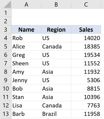
The first step is to insert a text box where you can type a text string and it will use it to filter the data (while you’re typing).
Below are the steps to insert the text box:
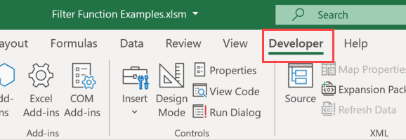
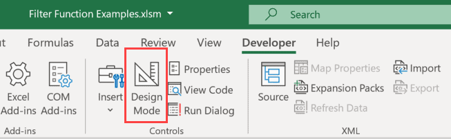
- Click the Developer tab.

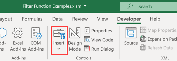
- In the Control group, click on Insert.
- Click on the Text Box icon in the ActiveX Controls

- Place the cursor anywhere in the worksheet, click and drag. This will insert a text box in the worksheet. You can place this text box wherever you want and can also resize it.

In case you don’t see the Developer tab in the ribbon (in Step 1), right-click on any of the tabs and click on ‘Customize the Ribbon’. In the Excel Options dialog box that opens, check the Developer option in the right pane and click OK. This will make the Developer tab visible in the ribbon.
Now that we have the text box in the worksheet, the next step is to connect it to a cell in the worksheet so that when you type anything in the worksheet, it will also automatically be entered in a cell.
This will allow us to use the value in the cell to filter the data.
Below are the steps to link the text box to a cell:
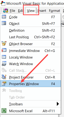
- Double-click on the text box. This will open the VB Editor.
- Click the View option in the menu and then click on Properties Window. This will show the Properties Window Pane for the text box.

- In the properties window, come to the Linked Cell option and enter F1. This is the cell that we are connecting to the text box

- Close the VB Editor
- Go to the Developer tab, and click on the Design mode. You will notice that it turns from dark gray to light gray (indicating that it’s not enabled now).

Now, when you enter any text in the text box, you will notice that it appears in cell E1 in real-time (as you’re typing)
Now that we have linked the text box to a cell, the last step is to filter the data based on the value in the text box (which in turn would be the value in cell E1)
For this, we need to enter the FILTER formula in cell E4, so that results are filtered and shown there.
Below is the formula that will now filter the results as soon you can enter anything in the text box:
=FILTER(A4:C13,ISNUMBER(SEARCH(E1,B4:B13)))
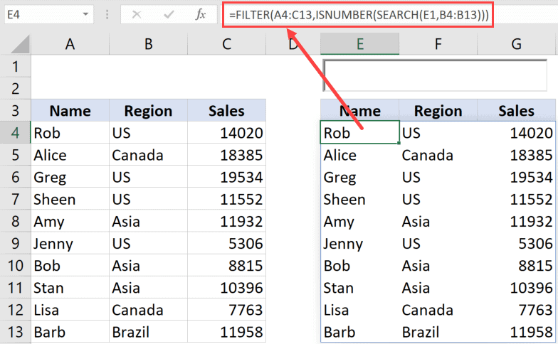
The above formula uses the FILTER function with the array as the original dataset and the condition uses the SEARCH formula.
The SEARCH formula checks whether the value entered in the text box (which also automatically gets entered in cell E1) is there in the cells in column B or not. All the cells that have the text will return a number and those that don’t will return the #VALUE! error.
The ISNUMBER function is used to get TRUE if there is a match and the cell returns a number, and FALSE is it returns the error.
Based on this condition, the data is filtered as you type.
Note that this formula checks whether the text string entered in the text box appears in the cells in column B or not. For example, if you enter ‘a’ in the text box, it would return all the records for Canada, Asia, and Brazil.
The position of the text string in the cells in column B is not checked.
In case you want to have the text string (that you enter in the search box) at the beginning only, you can use the below formula instead:
=FILTER(A4:C13,LEFT(B4:B13,LEN(E1))=E1)
Now when you enter A in the search box, it will only give you records for Asia.
If you’re not using Office 365 and don’t have access to the FILTER function, you can still create the ‘filter as you type’ search box in Excel.
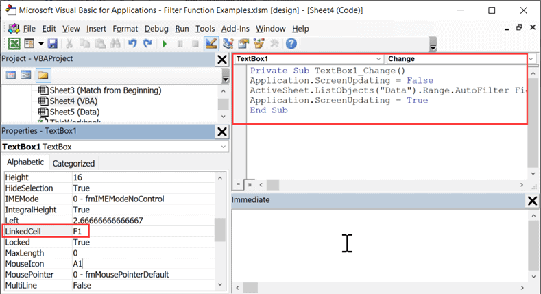
This can be done by using a really simple VBA code mentioned below:
Private Sub TextBox1_Change()
Application.ScreenUpdating = False
ActiveSheet.ListObjects("Data").Range.AutoFilter Field:=2, Criteria1:= "*" & [A1] & "*", Operator:=xlFilterValues
Application.ScreenUpdating = True
End Sub
To use this code, you will have to first insert the text box in the worksheet and then add this code for the text box.
But the first step is to convert the data into an Excel table. While you can use this code without converting the data into an Excel table, it will be easier when the data is in Table as it becomes easier to refer to in the VBA code.
Below are the steps to convert the data into an Excel table:
- Select any cell in the dataset
- Hold the Control key and press the T key (or Command + T if you’re using a Mac).
- In the Create Table dialog box that opens, check whether the range is correct or not.
- Click Ok
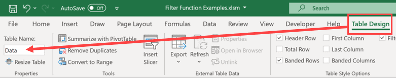
- Select any cell in the Excel Table
- Click on the ‘Table Design’ tab
- Change the name of the table to Data. You can use any name you want, but make sure to use the same one in the VBA code as well.

Below are the steps to insert the text box in the worksheet:
- Click the Developer tab.
- In the Control group, click on Insert.
- Click on the Text Box icon in the ActiveX Controls
- Place the cursor anywhere in the worksheet, click and drag. This will insert a text box in the worksheet. You can place this text box wherever you want and can also resize it.
Now that you have the text box in the sheet, you need to connect to a cell and then add the VBA code to the text box code window.
Below are the steps to do this:
- Double-click on the text box. This will open the VB Editor.
- Click the View option in the menu and then click on Properties Window. This will show the Properties Window Pane for the text box.
- In the properties window, come to the Linked Cell option and enter F1. This is the cell that we are connecting to the text box
- In the code window of the Text Box, copy and paste the above VBA code

- Close the VB Editor
- Go to the Developer tab, and click on the Design mode. You will notice that it turns from dark gray to light gray (indicating that it’s not enabled now).
Now you have a text box that is linked to a cell and this cell is used in the VBA code to filter the data.
When you enter any text in the text box, you will see that it filters the table in real tile (filter the data as you type in the text box).
Note: Since the VBA code is executed every time you enter a character in the text box, this method could make your workbook slightly slow in case you have a large data set. In such a case, instead of using the code in the text box code window, you can use it in a regular module and then assign it to a button. That way, you can first type the text in the text box and then click on the button to filter the data.
So these are two methods you can use to create a dynamic filter in Excel (filter data as you type).
Hope you found this tutorial useful!
You may also like the following Excel tutorials:
- How to Clear Contents in Excel without Deleting Formulas
- How to Clear Filter in Excel? Shortcut!
- How to Hide Rows based on Cell Value in Excel
- How to Unhide All Rows in Excel with VBA
- How to Delete a Sheet in Excel Using VBA
- How to Select Alternate Columns in Excel (or every Nth Column)
- How to Select Every Other Cell in Excel (Or Every Nth Cell)
- How to Paste in a Filtered Column Skipping the Hidden Cells
-
— By
Sumit Bansal
Excel Filter is one of the most used functionalities when you work with data. In this blog post, I will show you how to create a Dynamic Excel Filter Search Box, such that it filters the data based on what you type in the search box.
Something as shown below:

There is a dual functionality to this – you can select a country’s name from the drop-down list, or you can manually enter the data in the search box, and it will show you all the matching records. For example, when you type “I” it gives you all the country names with the alphabet I in it.
Download Example File and Follow Along
Watch Video – Creating a Dynamic Excel Filter Search Box
Creating a Dynamic Excel Filter Search Box
This Dynamic Excel filter can be created in 3 steps:
- Getting a unique list of items (countries in this case). This would be used in creating the drop down.
- Creating the search box. Here I have used a Combo Box (ActiveX Control).
- Setting the Data. Here I would use three helper columns with formulas to extract the matching data.
Here is how the raw data looks:
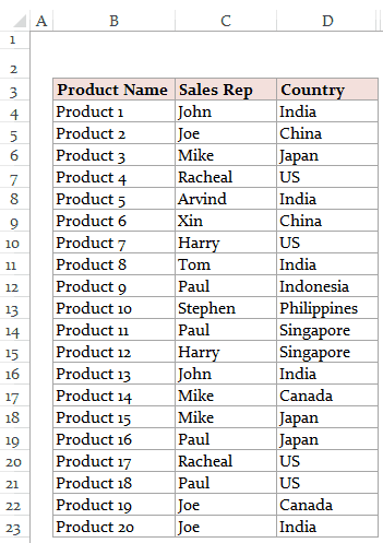
USEFUL TIP: It is almost always a good idea to convert your data into an Excel Table. You can do this by selecting any cell in the dataset and using the keyboard shortcut Control + T.
Step 1 – Getting a unique list of items
- Select all the Countries and paste it into a new worksheet.
- Select the country list –> Go to Data –> Remove Duplicates.

- In the Remove Duplicates dialogue box, select the column in which you have the list and click Ok. This will remove duplicates and give you a unique list as shown below:

- One additional step is to create a named range for this unique list. To do this:
- Go to Formula Tab –> Define Name
- In Define Name Dialogue Box:
- Name: CountryList
- Scope: Workbook
- Refers to: =UniqueList!$A$2:$A$9 (I have the list in a separate tab named UniqueList in A2:A9. You can refer to wherever your unique list resides)


NOTE: If you use ‘Remove Duplicates’ method and you expand your data to add more records and new countries, you will have to repeat this step again. Alternately, you can also you a formula to make this process dynamic.
See Also: How to use a formula to get a list of Unique items.
Step 2 – Creating The Dynamic Excel Filter Search Box
For this technique to work, we would need to create a ‘Search Box’ and link it to a cell.
We can use the Combo Box in Excel to create this search box filter. This way, whenever you enter anything in the Combo Box, it would also be reflected in a cell in real-time (as shown below).

Here are the steps to do this:
- Go to Developer Tab –> Controls –> Insert –> ActiveX Controls –> Combo Box (ActiveX Controls).
- If you do not have the Developer Tab visible, here are the steps to enable it.

- If you do not have the Developer Tab visible, here are the steps to enable it.
- Click anywhere on the worksheet. It will insert the Combo Box.

- Right-click on Combo Box and select Properties.
- In Properties window, make the following changes:
- Linked Cell: K2 (you can choose any cell where you want it to show the input values. We will be using this cell in setting the data).
- ListFillRange: CountryList (this is the named range we created in Step 1. This would show all the countries in the drop down).
- MatchEntry: 2-fmMatchEntryNone (this ensures that a word is not automatically completed as you type)

- With the Combo Box selected, Go to Developer Tab –> Controls –> Click on Design Mode (this gets you out of design mode, and now you can type anything in the Combo Box. Now, whatever you type would be reflected in cell K2 in real time)


Step 3 – Setting the Data
Finally, we link everything by helper columns. I use three helper columns here to filter the data.
Helper Column 1: Enter the serial number for all the records (20 in this case). You can use ROWS() formula to do this.
Helper Column 2: In helper column 2, we check whether the text entered in the search box matches the text in the cells in the country column.
This can be done using a combination of IF, ISNUMBER and SEARCH functions.
Here is the formula:
=IF(ISNUMBER(SEARCH($K$2,D4)),E4,"")
This formula will search for the content in the search box (which is linked to cell K2) in the cell that has the country name.
If there is a match, this formula returns the row number, else it returns a blank. For example, if the Combo Box has the value ‘US’, all the records with country as ‘US’ would have the row number, and rest all would be blank (“”)
Helper Column 3: In helper column 3, we need to get all the row numbers from Helper Column 2 stacked together. To do this, we can use a combination if IFERROR and SMALL formulas. Here is the formula:
=IFERROR(SMALL($F$4:$F$23,E4),"")
This formula stacks all the matching row numbers together. For example, if the Combo Box has the value US, all the row numbers with ‘US’ in it get stacked together.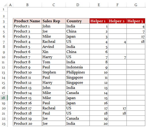
Now when we have the row numbers stacked together, we just need to extract the data in these row number. This can be done easily using the index formula (insert this formula in where you want to extract the data. Copy it in the top-left cell where you want the data extracted, and then drag it down and to the right).
=IFERROR(INDEX($B$4:$D$23,$G4,COLUMNS($I$3:I3)),"")
This formula has 2 parts:
INDEX – This extracts the data based on the row number.
IFERROR – This returns blank when there is no data.
Here is a snapshot of what you finally get:
The Combo Box is a drop down as well as a search box. You can hide the original data and helper columns to show only the filtered records. You can also have the raw data and helper columns in some other sheet and create this dynamic excel filter in another worksheet.
Download the Dynamic Excel Filter Example File![]()
Get Creative! Try Some Variations
You can try and customize it to your requirements. You may want to create multiple excel filters instead of one. For example, you may want to filter records where Sales Rep is Mike and Country is Japan. This can be done exactly following the same steps with some modification in the formula in helper columns.
Another variation could be to filter data that starts with the characters that you enter in the combo Box. For example, when you enter ‘I’, you may want to extract countries starting with I (as compared with the current construct where it would also give you Singapore and Philippines as it contains the alphabet I).
As always, most of my articles are inspired by the questions/responses of my readers. I would love to get your feedback and learn from you. Leave your thoughts in the comments section.
Note: In case you’re using Office 365, you can use the FILTER function to quickly filter the data as you type. It’s easier than the method shown in this tutorial.
You May Also Like the Following Excel Tutorials:
- Highlight Matching Data Using Conditional Formatting – Dynamic Search.
- Create a Search Suggestion Drop Down List in Excel.
- Using Advanced Filter in Excel.
- How to Extract a Substring in Excel (Using TEXT Formulas).
- Creating a Drop Down Filter to Extract Data Based on Selection.
- How to Filter Cells with Bold Font Formatting in Excel.
- Highlight Rows Based on a Cell Value in Excel.

Get 51 Excel Tips Ebook to skyrocket your productivity and get work done faster
187 thoughts on “Dynamic Excel Filter Search Box – Extract Data as you Type”
-
Hi, how do i get the helper columns to automatically update when i add to my MasterData list when the helper columns are hidden?
Thanks -
Hey Hi There, this does not work in large data it takes too long to find the result is there any other way to do it?
My data is of 5lks -
Hi,
what if i want to filter only unique record only? lets say in my data against the country japan “Product 7” is coming for 7 times but i want to filter it only one time . is it possible?
-
What is the workaround to the ActiveX to reproduce this result? I’m working in a Mac environment and AX is problematic.
-
Brilliant Idea, It helped me a lot, I was looking for a similar solution
Thank you -
Hi Sumit
Thank you for this excellent post.
I have a question regarding sub-query within the attribute.For example if you want to see product category from both India AND China how do you change the equation?
In this case we are trying to separate group of country and applying filter on them.
-
Great article that I have immediately put to use! How would I have the cursor default to being inside the combo box when the workbook is opened? Thanks
-
This is a brilliant tutorial with a very effective final result. Thanks for laying this out. I’ll be using this over and over again, I’m sure. FANTASTIC!
-
Excellent Video.
I was thinking how it would be possible to apply this advance filter and then have the option to input data into the filtered products.Example I filter for India, it bring up 4 result and then I want to input data to the results. More like i’m filtering the actual entire row of the result?
You response will be greatly appreciated.
-
hi, I have been using this dynamic filter system for years and it works brilliantly!!!.
One thing that was not needed was the drop down choice to be filtered, but
recently I have re-used this idea and again it works perfectly but….. this time the drop down filter to choose just a letter and it filter the results would be wonderful, but it just doesn’t work. I have downloaded the excel file and have copied everything to the letter but it just chooses the full name of the selection. Can anyone help. -
Hi Sumit,
I’ve found your video extremely useful, but like a lot of others I’m struggling to apply your formula to multiple searches/filters/conditions. I’ve seen you’ve shared a dropbox link for this solution but they have expired. Is it possible to please create another link or to comment in an example of this formula – this would be much appriciated.
Many thanks,
Jack
-
Hi There,
It really helped me do the search bar and it works fine,
however, my data is huge and it takes lot of time to get the output and it keeps calculating.
Kindly suggest on the concern. -
You are really good
-
How do I create this for multiple excel filters? Let’s say, I want to put in a second filter.
-
Hey Bradley – did you figure this out? I am trying to do the same
-
Hey, no I didn’t figure it out; hoping someone would lend a hand
-
It says above it can be done ‘exactly following the same steps with some modification in the formula in helper columns.’
Can anyone help??
-
-
-
I did get this to work with multiple filters. Use the search for multiple selections (Column Helper 2 – apply for each sort field) to come up with the data columns, and then use a separate column to call out where the various columns all have the same data. I did three helper columns with a sort of “if Helper 1 = Helper 2 = Helper 3 then show value in Helper 1”. Then I did the sort in Helper 3 off of the new column and it worked.
I hope that makes sense…
-
-
how if searching in multiple sheets
=IFERROR(INDEX(‘DAY1′!$B$6:$O$55,’DAY1’!$S6,COLUMNS($B$10:B10)),””)
day 1 = 1 sheet up to 31 sheet -
I like your post it is very informational. Kindly also make post to use this search filter in vba form
-
Another variation could be to filter data that starts with the characters that you enter in the combo Box. For example, when you enter ‘I’, you may want to extract countries starting with I (as compared with the current construct where it would also give you Singapore and Philippines as it contains the alphabet I).
I would love to know will I do the above statement. and btw thankyou for the video it really helo me a lot. the only thing that i need to do is the statment above.
I hope you will answer this
-
So effective… Thank you so much !
One improvement would by to allow us to search for multiple words. -
What if i would like to have the entire spreadsheet to be filtered to only extract data with everything that contains “la” or “east”. This formula only allows for data from a specific column. How can this be accomplished?
-
hi
please I have different sheet each one of them have the same think just different company name. i want to have as in this exemple but result in an other sheet and also the data coming from different sheet
thanks -
I know this is old, but I know too that a lot of people still uses this topic. It’s so useful! But I’d like to know if there is any way to make the search box better, I mean, searching Products, Sales Rep and Countries. Not ONLY contries. Thanks!
-
hi
first, thank you for this excellent work :I need, please your help if you can.
I want to know I want to create this filter first with more than 15 worksheets and each one having the same column and rows information.
I want to create a comparison tool, as if, I enter for example item number or name will give me a grill with what I need in a unique worksheet as an output.
Here is what I have :
1- 15 worksheets: each worksheet, it’s for a specific company, each sheet has the same thing: ex:
item name, prices, capacity, our prices, margin, etc..2- I want to make a search ( as you did in the box you create ) when I search for example by name:
*** My result expected: will give a table with the less price first and which company is associated with.
3- is it possible to do with excel, if not can you guide me please, which program I can need to use is it a database +VB or what exactly, please.
Thanks a lot.
-
sorry,its doesn’t work over 313 rows,what i should do?
-
Can I make it show no result until/unless I type something in the search box?
-
Can a search box be created in a second sheet using the data from sheet1?
I have about 2500 line items (Inventory) and 7 header columns. I currently use Conditional formatting but the problem is scrolling down the page to see what is highlighted.-
Yes, you can.
Make these “helpers” in the sheet where all the data is.
Then, in the secondary sheet, make a table with Filtered Data.
=IFERROR(INDEX((dataSheet!$B$4:$D$23000);(dataSheet!$G4);COLUMNS(showSheet!$A$4:A4));””)
-
-
Is there a way to then be able to sort through this list? When I sort, some blank rows appear
-
Sort Z>A not A>Z
-
-
I need to use a dynamic filter text for online usage, with a shared website in my company. How can I use ActiveX Dynamic filter this way?
-
How can I do this if I don’t have a designer license?
-
Would it be possible to set up 2 columns, where the first column has multiple looks for “this” AND “that”, and the second column has fields that looks for “this” OR “that”, and return the results in the same column?
-
Very nice
-
Extremly super admin.. i appreciate it a lot. thank you so much.
-
can you do the filter without using helper columns? i mean, filtering the data table?
-
How do you make it so that hyperlink would stay intact in your search results?
-
how can i provide security for this file.i mean we have a cleint list.the flle shall be available for everyone in office.i can protect workbook with a password. but search bar also getting password protection. what can i do
-
hi, could we make this filter but with additional conditions instead of just 1 condition?
-
Hello,
I have successfully completed this; however, one of my columns with information the populates contains hyperlinks to documents on the computer. Right now these hyperlinks are only showing up as text. I would like the link to be retained when it appears in the search results, can you help with this?
-
Hi Sumit, can you tell me how can I customize the text search to show only the specific text I am looking for? Current formulas return any text that contains what was entered in the text box.
Thank you for your help,
Enna-
I’m also having this problem. Any help would be appreciated!
-
-
hi…
if there are multiple rows then what should be done in helper coloumns…. do i setup the helper 4 row and which formula i have to enter…
please do needful help -
This works great for my needs! I would like to hide the dynamic list while the search box is empty and only show the results. Is there a way to do this?
-
I like the idea (and I’m guessing this is pretty old) but this is the most round about way I’ve ever seen to accomplish this. What you really want is to simply work the autofilters via the combobox’s change event. if you need to view your filtered data on a separate sheet then simply copy the filtered range to it. No need for helper columns or vlookup/index formula’s either. You could also use a dynamic range in VBA and forget about the static named range altogether.
Just my 2cents…-
Hi SM177y
can you please elaborate on this?
I think you are referring to manage large number of data rows
I have around 10K rows and the original equation in this post is little slow.how can i improve this?
-
-
Hello. This is a great tutorial and is just what I was looking for. However, I’m stuck on Helper 3. In the YouTube video you mention something about adding ROWS. I can’t see the formula because the video is a little blurry. In the instructions above, there is no mention of rows. When I follow the instructions above, I’m not getting my numbers stacked in Helper 3.
-
Hello.. The ROWS function is used in Helper Column 1. The formula used in cell E4 is =ROWS($B$4:B4) and then copied for all the remaining cells in the column. You can also download the example file and see the exact formula in it.
-
-
Hi Sumit, just to check can we select two filters like maybe one box for both country and name or two boxes , one for country and one for name. How would the excel sheet formula be like? Thanks in advance
-
I am still a relative novice with excel, so forgive me if my question seems silly. I was fine until I got to creating the index. When I try to drag the formula down and to the right, it changes the formula in the other boxes in such a way that the search doesn’t bring up the proper information. Basically the formula changes by shifting the area of information either down a row or one column to the right. Is there a way to prevent it from changing anything other than what is necessary for accuracy so I don’t have to manually go in and fix it?
-
Straight forward with clear explanations! Sambit you are an excellent trainer 🙂
-
This is brilliant, thanks a lot for posting it!
-
too good, but this formula only on 20 cell i need it on 2k cell please help me!
-
i need this formula, but its work only with 20 cell in need it till 2k cells. please help me?
-
Following this guide, to use it on a larger data set, you would only need to redefine the named range to include however many rows you need….But if you read my other comment and do a little Googling, you’ll find much easier, faster, and more efficient ways to accomplish this that aren’t bound to any static range.
-
-
Is there a way how I could add more than 1 dynamic filter in a sheet? Let’s say first I sorted all which were for India, and then via second one I need to sort only Sales Rep John within India. Thanks in advance. Emil
-
Many thanks for this. I was able to follow your very clear explanations. Works remarkably well. I’d like to add a button to clear the search field. I wonder if you would mind sharing any suggestions?
-
Thanks a lot
-
Hi Sumit,
I would like to make dynamic books title list with the help of this formula, can you suggest further options to me e.g. – once a user will get the data after applying drop down option after this can he directly email the outcome to clients or save the outcome in PDFemail – varunsharma16@gmail.com
-
Hi, Plz give me the two filters in same excel file and its not working in office 2007.
Plz help me with sample file
-
-
-
Thanks it works!
-
-
-
-
Hi Summit – I fixed the issue with the table populating when using the combo boxes. I do have two other questions. When I use the Combo boxes for filter it includes any results that has similar spelling, but I just want it to show the “Brand” I have selected.
How do I update Helper 2 formula: =IF(AND(ISNUMBER(SEARCH($M$2,B4)),ISNUMBER(SEARCH($L$2,C4)),ISNUMBER(SEARCH($K$2,D4))),F4,””)
My other question is how can I show no results when no combo filter box has nothing selected?
Thank You! Great tutorial.-
Use the exact formula instead of search. Use the following formula in helper column 2: =IF(EXACT($K$2,D4),E4,””)
-
Your above finding was really helpful for my report with multiple filters. This is what I was looking for. Appreciate your contribution 🙂
-
I’m having issues with the Helper Column 3 with this formula, where nothing is displayed / organised despite the filters being met. Any ideas?
-
-
-
Hi Sumit, would you please share the formula to include up to 30 conditions again please? I can’t seem to be able to access the file via the dropbox link above. It would help very much!
Thank you!! -
Great idea. My list fill range does not seem to work. When I type in the Name of my unique list, it disappears when I hit enter. Any ideas? Thanks!
-
I was able to replicate the issue using your demo file. It seems to fail if you turn the unique list into a table and use the =Tablex[ColumnY] function. Pretty frustrating that Excel does that. I prefer to use the table functions as my arrays/lists rather than a range, since the unique list may change over time. Any ideas of a workaround? Thanks!
-
This is a known issue with Excel 2013 being unable to directly refer to a table name. Instead we have create another surrogate name that simply refers to the first. Then ListFillRange will accept it. source http://www.contextures.com/excelworksheetcomboboxes.html
-
-
-
Hello Sumit, thank you for your wonderful and very helpful tutorial. Question, I have certain questions that are highlighted but when they are extracted they’re no longer highlighted, how can I keep the questions in the same style?
thank you for your amazing knowledge. -
हिन्दी में बताइए
-
This is brilliant! Thanks for the sharing! Very useful!
-
This was great Sumit! Very helpful. I ran into one problem and was wondering if you knew a quick fix. If it was mentioned already in the comments, please let me know and I’ll go find it. In my list, I have terms such as NBC, MSNBC, CNBC, etc. When I do the drop down selection for MSNBC, I only get results for MSNBC (which is good!) However when I do the drop down selection for NBC, I get results for anything related to NBC (NBC, MSNBC, CNBC, NBCSN, etc). Is there a way for me to isolate just NBC? Thanks
~Brian -
Hi there, can I embed this feature on my website?
-
Great article Sumit. Thanks for sharing 🙂
I’ve just discovered a pretty good video where the search filter works dynamicaly by hiding the rows. Looks very nice and useful. Moreover, there is a download link below the video, so you can try it immediately.
Maybe you will find there some new ideas..
-
thanks yu, you are really helping me a lot.. keep up your good work. god of excel 🙂
-
-
Hi… Thanx for the great post…it was really helpful !!!
I want to do something similar, but rather than filtering on the column i want to filter by row.
i.e. You are showing a row if it the cell has the particular value, I want to show the columns if the cell in it has the particular value. I am able to write formulas for populating the helper columns.
But am stuck with the last one to populate the final set.
Can you please help with this? -
Thank you for the video. What if I want to extract any data that I type in the combo box, what would the formula be? Thanks.
-
Is there a way to auto fill repetitive data like name and address?
-
-
Thanks Sumit for the reply and pointing me to the right topic. I will check out the link.
-
I did check the link but it does not suit what I was looking for. This is the actual scenario what I am looking for maybe you can point me to the right topic. We have to input name of companies to Excel based on the Invoice issued, the name would occur several times. Together with the name there is assigned Tax Identification Number that would be inputted beside the company name. I would appreciate any help.
-
-
-
Fantastic demo, well written. I’m a little confused why you need to create a unique table, why not dump all your raw data on one sheet (in my case, priority, alarm, information, support team) and have another sheet do the search and display the relevant rows below ? This would (I think) be more universal and help more people. Just a thought, not by any means a criticism.
-
Thanks for sharing Miles.. Unique list is created for the drop down, so that there are no repetitions in that. If that’s not needed, that you can do away with the unique list step
-
-
Hello,
If I have dates in mm/dd/year (or some equivalent) how can I use the dynamic filter to search by month or year whilst keeping the date format?
Unfortunately even if the dates are formated to say the respective month it only searches in based off of what is in the formula box.
I look forward to your response.
-
Hi Sumit, thanks for this. It’s a great tutorial. I have a couple of further issues I’m hoping you can help me with. In my filtered results any cells that were left blank in the raw data now have a 0 (zero) in them. Is there a way to show the cells as blank in the filtered results? Also, some of the filtered cells contain hyperlinks. These are “live” in the raw data (if you click them they open the relevant page in your browser), but they are not live in the filtered data. Is there a way to make them live in the filtered data? Thanks for any help you can give!
-
hello, thanks for your post. but i noticed the first formula doesn’t work for me
-
HOW DO I SELECT ONLY ITEMS THAT START WITH THE CHARACTER I WANT. IF I ENTER “PH” I WANT TO RETRIEVE PHILLIP NOT ALPHOSO…YOU MENTION TWEEKING THE HELP BUT I’M NOT SURE HOW..
-
Hello. Thank you for the superb post. You saved me big time. But there’s a problem. The search box also filter the words that contain the words I search. For example, I search for “AN” and the rows with “CHANH” also appear. How can I set it so that only the exact word is filtered?
-
Hello Minh. You can do that by replacing the formula in Helper 2 with the following: =IF(AND(ISNUMBER(SEARCH($K$2,D4)),LEN(D4)=LEN($K$2)),E4,””)
Simply put this formula in F4 and copy for all the cells in that column.
-
-
Hi Sumit, Can you show how to add two filters, Country and Product? How can that be done?
-
-
Hello, Is it possible to take the range of the ‘Filtered Data’ section from one sheet to another?
If I copy the formula over and add the sheet name before the cell I can see all the current values, but it doesn’t appear to be dynamic and update like the information does on the original sheet.
any help is appreciated.
-
Hello JP.. You can get the filtered data in another sheet as well. Instead to adding the sheet name manually, I would suggest you reconstruct it from scratch (as shown in the tutorial). That way Excel will take care of the cell referencing and naming itself
-
-
Hi Sumit
This is a brilliant method for making a searchable staff telephone list. However, some of my cells in the range are blank, where there is either no extension or mobile, and they are showing in the search result table as 0. I have tried, without success, to add an if statement to weed these out and show them as blank cells. Is there a way to do this without causing the formula =IFERROR(INDEX($B$4:$D$23,$G4,COLUMNS($I$3:I3)),””) to throw up an error?
-
Hello Dawn.. Would be great if you could paste a screen shot of the data, or send me the data via email. I just want to make sure I give you the formula that suits your data. It can be done by tweaking existing formulas used in the template
-
-
Hi Sumit,
Thanks for sharing!
I am currently putting the dynamic filter and its data on a different worksheet. May I know if it is possible to also have a filter option to display “All the data”.
If I would like to have the option to choose “All Countries” from your example, how would I be able to do it?
-
-
When the combo box is empty it shows the entire result(s). Is there a way when the combo box is empty the results are blank?
-
Hello Rob.. change the formula in Helper Column 2 with the following formula: =IF(AND($K$2″”,ISNUMBER(SEARCH($K$2,D4))),E4,””)
Now when the combo box is empty, it will show no results
-
-
Hi Sumit, is it possible to search 2 items at the same time for example: all the US and the Canada ?
-
-
Hi Sumit – this is awesome! Just wondering if you’re able to help me out a little bit more?
I’m trying to do a version of this where the data is output to a second sheet (saves me from hiding & unhiding cells all the time).
I’ve managed to output the data to a sheet named UI (user interface) but now the search filter isn’t working. It’s probably something to do with how I’ve written the Formula’s, but I can’t figure it out.
I’ve attached screenshots showing the sheets and the formula’s being used. Any help would be much appreciated!
Cheers,
Jen-
Hello Jen.. Can you share the file (may be a dropbox or onedrive link). I can’t see snapshots here
-
-
This is super awesome ! One quick question: can we highlight the keywords in some color in the database as we type and it hits the match. Please let me know
-
-
I checked this one before, not working for me. I already have a dynamic filter using the formula what’s it’s shown here, now i want to color code only texts while typing using the same dynamic filter .. I have used 3 helper and the formula is the same what’s shown in this. Also I have created a front end where showing the search results but the color coding is not working. Don’t know why.
-
-
-
Sir, Thank you so much for the tutorial, you save my family’s business.
I do have a bit of question. Instead of country name like Japan, India, Singapore, I have a “group id” like 001, 01, 240, 24, 924. And I did >Define Name and all. But once I start using the combo box, “24”, the items of other group like 240 and 924 would come along.I guess it has something to do with The helper 2 column “=IF(ISNUMBER(SEARCH($K$2,D4)),E4,””)”
Could you please help me to search the result of the exact value? Thank you so much !-
Hello Seebear.. You can do that by changing the formula in Helper Column 2 to =IF($K$2=D4,E4,””)
-
-
hi i m sumeet , sir i want to know that can i edit the data selected from the drop down list on real time , for eg. i have selected sumeet as my name from the drop down list & i want to add singh as my surname after my name on real time basis
-
This was so helpful. Thank you. I had been banging my head all week trying to do this on my own.
Only issue I encountered is after selecting the item from the Combo list, sometimes the selection just disappears – i.e. the combolist seems to just clear itself. Not sure what is going on there. Do you have any idea what could be causing this please?
-
can we add 3 or 4 columns in data and shown in filtered data
-
Hello Sumit, thanks a lot very helpful site!! I have been trying for days now without getting any solution. Is there a way to edit the filtered values? for example I type Japan. Then once I have the filtered results I go and change/update the Sales Rep name?
-
hi. if I have 6 columns, then i will be having 6 helper?? pls answer. thanks
-
hi Sir,
i have tried it on my datasheet using the same formulas but it seen like i cant filter the information what i want.
can you able to see what wrongs with my formula?thank you in adance
-
Hi,
As i mentioned in the comments below. I’ve got a pretty large dataset for which this solution really struggles. and takes good few seconds to filter through data. I’ve just read about INDEX MATCH formula – so was wondering if this type of dynamic search could be achieved using INDEX MATCH formula, which should be most probably quicker than the INDEX you have used here. Please advise.
Thank youp.s. more about INDEX MATCH benefits: http://www.mbaexcel.com/excel/why-index-match-is-better-than-vlookup/
-
Hello Sumit,
Thank you so much for uploading this video. Is there any way to show the search result blank if there is no data in the combobox ?
-
Hello Siddhartha.. Thanks for dropping by and commenting. You can do this by changing the formula in 2nd helper column to: =IF(LEN($K$2)=0,””,IF(ISNUMBER(SEARCH($K$2,D4)),E4,””))
Paste this formula in F4 and drag it down.
-
Hi Sumit,
Thanks for your sharing, if the data table have a blank in somewhere cell, it doesn’t count this row, any formula can solve it?
-
-
-
Keep going, i am a fan of this website.. Gaurav Negi
-
Thanks for commenting Gaurav,, Glad you like the tutorials here 🙂
-
-
Hi Sambit,
Regarding the variations: I’m wondering if it’s possible to have more than two conditions/filters? I can’t seem to figure out the correct formula.
Thanks!
-
-
Hi again Sumit,
I’ve downloaded that version and applied the formula to my spreadsheet. It works perfectly for two conditions, but I can’t figure it out for more than two. Is this possible? Sorry if this isn’t clear!
-
-
AMAZING! Thank you so much for your quick response. Is there a maximum condition limit, or can you use as many conditions as you like? Thank you again!
-
Glad it helped.. The number of conditions depends on the data, In this case, we have 4 columns of data, so there could be 4 conditions. AND formula can handle a maximum of up to 30 conditions
-
I added another condition and it worked. Thank you so much again for your help, it’s much appreciated!
-
Hi Sumit, would you please share the formula to include up to 30 conditions again please? I can’t seem to be able to access the file via the dropbox link above. It would help very much!
Thank you!! -
Gr8, but Combo Box 2 is drop down list is carrying sales rep data, though in case I type any name of product category, it’s ok.
-
-
-
-
-
Nice,works well, but unusable with big tables, takes 5 min to filter a 12k row table on a Quad Core i5 with 4G RAM. I am aware this is not the intended use, just want to inform others who want to give it a try 🙂
-
Hi.
I’m in the same situation as posted above. I’ve got a file of 15 000 rows and the list is constantly growing. I’ve tried the formula with helper columns and all works great, apart that it takes around 1-3 seconds to generate a list from my query. Also the way i made a formula is to output the data to another sheet as a summary instead of seeing all raw data, so it looks really need. I’ve also tried the same solution with the 1 000 entries and that returns data as i type. I’ve got i5 6 GB laptop and it really struggles with the large database (15k rows). Is there another way of making the same dynamic search that wouldn’t put so much pressure on processor and would return data as i type?
Also big thanks for trumpexel for such a great solution.
-
-
Hi there 🙂 Suppose I have hyperlinks instead of text data in the specific columns, how do I retain the hyperlink and not extract the data as text after the search
-
-
ahh ok thanks for the prompt reply!
-
Club the two? I have web links in the “Sales Rep” Column. How do I get it to retain the hyperlink after it has been searched? This has been very helpful so far. Thanks!
-
-
-
I have a huge data approx. 50,000 rows and i want to filter it with search box as i start typing in the search box the data starts to filtering but i am failed to do it.
Your example is too good but I don’t want to use “INDEX” formula.
Please help me out.-
Hi.
I’m in the same situation. I’ve got a file of 15 000 rows and the list is constantly growing. I’ve tried the formula with helper columns and all works great, apart that it takes around 1-3 seconds to generate a list from my query. Also the way i made a formula is to output the data to another sheet as a summary instead of seeing all raw data, so it looks really need. I’ve also tried the same solution with the 1 000 entries and that returns data as i type. I’ve got i5 6 GB laptop and it really struggles with the large database (15k rows). Is there another way of making the same dynamic search that wouldn’t put so much pressure on processor and would return data as i type?
Also big thanks for trumpexel for such a great solution.
-
-
Hi Sumit,
You wrote this “You can try and customize it to your requirements. You may want to create 2 filter instead of one. For example, you may want to filter records where Sales Rep is Mike and Country is Japan. This can be done exactly following the same steps with some modification in the formula in helper columns.”
Could you please tell me what changes to make in helper columns to make 2 filters work?
Thanks a lot!
Kindly let me know.
Best Regards,
Karthik-
-
Thanks Sumit, i tried that, but it gives me a message “we found one or more circular references that might cause your formulas to calculate incorrectly”. is there something I can look out for to resolve this problem?
-
Hey Karthik.. Are you talking about the file I shared, or something you created? The file I have shared works fine on my system. I checked and there are no circular reference errors. If it’s a file you have created, kindly share with me and I can have a look
-
-
-
-
You can try and customize it to your requirements. You may want to create 2 filter instead of one. For example, you may want to filter records where Sales Rep is Mike and Country is Japan. This can be done exactly following the same steps with some modification in the formula in helper columns.
Sumit, Could you please tell me how to use 2 filters, i.e. what changes to make in the helper columns?
Thanks -
hi, this is very useful for my task. But I need one that can hyperlink also. Does this dynamic filter can be linked to other file such as pdf file? For example, if I click product 1 in the filtered table, I expect that it will open another file consists of product 1 data. Is it possible? Thanks
-
-
I guess I can’t link it to other file like .doc? only to data in the same workbook
-
What if I want to Hyperlink to a website?
-
-
-
Yes . I have a database where there are 50 columns and each column has
10000 rows , with new entries being added each day . I want 50 dynamic
filters on each column so that i dont have to scroll the page for
applying filters on each column . As i want to filter data with
combination of any number of columns , i was looking for multiple
dynamic filter . Basically i want to use normal filters to filter data ,
with the exception that i can place the combobox as per my convenience
. Also if you can tell any technique wherein when I type the data in
dynamic filter it gives a google type search dropdown also , it will be most
helpful . Thanks -
this was really helpful .. can anyone tell how to make more than one dynamic filter in this
-
Glad you liked it.. What do you mean by more than one filter. Are you looking for more than one criteria?
-
-
Great Bansal sahab
-
Thanks for commenting.. Glad you liked it 🙂
-
-
hi Sumit,
two days back only I came across your site and just looking through..it makes me wonder!!
Keep on keeping On.Amal
-
Hello Amal.. Welcome to Trump Excel and Thanks for commenting.. I am really glad you found the website useful 🙂
-
-
Hey, great idea and implementation. I might use it at school to teach the kids a few tricks. Can all of this be done with a text field instead of drop-box?
-
Thanks for commenting and glad you liked it 🙂 I am afraid I not aware of any way to do this without combo-box. The benefit for combo-box is that it makes the data entry dynamic, which instantly gives you results.
-
-
This is worked perfect! I have a table with 830 rows that displays totals at the bottom of each column; and each filter option will result in about 200 rows. The problem that I have now is that I have to scroll all the way down to row 831 in order to see the totals. This document will also be printed by end users and I would like to avoid the extra blank papers. Any suggestions will be highly appreciated.
-
Hi Michelle.. you can try this formula:
=IF(AND(G3″”,G4=””),SUM($G$4:G4),IFERROR(INDEX($B$4:$D$23,$G4,COLUMNS($I$3:J3)),””))
I have made it based on the data set I have provided in the download file (assuming Column C has numbers)
-
-
Very cool
-
Thanks Buddy.. Glad you liked it 🙂
-
-
It is really helpful
-
Thanks for the comment Uday.. Glad you liked it 🙂
-
Thanks for commenting Uday..Glad you liked it 🙂
-
Thanks alot for this great video , it helped me alot , God bless you
-
-
-
Hey, I did it without Helper and Array. For intermediate level, it’s bit complex 🙂
{=IFERROR(INDEX($B$2:$D$21,SMALL(IF(ISNUMBER(SEARCH($U$1,$D$2:$D$21)),ROW($D$2:$D$21)-1,””),ROW()-4),COLUMNS($L$4:L4)),””)}
-
Hello Deepak.. Thanks for commenting and sharing the formula 🙂
-
Hi Deepak, can you maybe brake your formula down into smaller segments so i can understand what and how you did it. Also i’m trying to find a way to work with 15k lines of dataset which Trumpexel is not really coping well with as it takes 3-4 seconds to give the results on i5 6GB RAM processor. So i wonder if your formula would be any quicker as it wouldn’t need helper colums. please advise.
Thank you-
dragging the array formula till 15k row will make the excel sheet slow..
-
-
Hello Deepak, i’m really interested in seeing the rest of your formula here, for some reason it’s cutting it off after ROW($D$2:$D$21)-1,””),
I know it was a long time ago, but if you could possibly reply with the rest of the formula i would really appreciate it!
-
Nevermind, it appeared when I opened in a different browser, thank you!
-
Thanks Randy, you know it takes time to understand my own complex formula 🙂 lol …
-
-
-
Hey Deepak Could u share your excel sheet. Your formula is little bir confusing
-
Its difficult to find the excel file, what i have done is – i have incorporated all the helper formula in one formula..so it became big.
-
Sure but i can’t upload the excel file here, can you please share your Email Id so that i can send it to you.
-
-
Sent
-
-
-
-
Hi Deepak, would you be able to send me a copy of the corresponding excel file please to help understand your formula a bit better? Thanks in advance!
-
Pls share your email so that I can send you the file.
-
-
Do you know how can I multiple excel filters with your formula?
Thank you,
-
-
Really it’s great…….
-
Thanks for commenting Sambit.. Glad you liked it 🙂
-
Hello Bansal,
i’m new on the forum. i looking for a way to do exactly what you describ in this topic.
from the bebening, it works well. but when it come to apply the formulla, it became confused for me. the formula doesn’t work on my side.
it come with mistake from the helper column 2 :=IF(ISNUMBER(SEARCH($K$2,D4)),E4,””)
can you help me please.
will be gratfullIsaac
-
-
Comments are closed.
I have a excel worksheet with thousands of records. I would find/implement a Search as you type application on Excel. Are there any plugins for Excel that does this? Or do I need to use VB to code this. If so, how do I go about it? Thanks.
For example, I want to highlight and jump to first matching cell as user types in the search term in a text box
asked Feb 11, 2009 at 3:54
![]()
qwertyuuqwertyuu
1,0551 gold badge10 silver badges14 bronze badges
2
This is very simple to do using VBA and a form…
Enter the following in a regular Module:
Public Sub FindAsYouType()

    UserForm1.Show (False)

End Sub
And use something like the following in your code:
Private Sub txtFind_Change()
    Dim strFind As String
    Dim wks As Worksheet
    Dim varFound As Variant
    Set wks = ActiveWorkbook.ActiveSheet
    Set varFound = wks.UsedRange.Find(Me.txtFind, , , , , , True)
    If Not varFound Is Nothing Then varFound.Select
End Sub

Private Sub txtFind_KeyDown(ByVal KeyCode As MSForms.ReturnInteger, ByVal Shift As Integer)
    If KeyCode = vbKeyReturn Then Unload Me
End Sub
I hope this helps someone else out there! 
answered Jan 27, 2011 at 6:46
![]()
Excel for Microsoft 365 Excel for Microsoft 365 for Mac Excel for the web Excel 2021 Excel 2021 for Mac Excel 2019 Excel 2019 for Mac Excel 2016 Excel 2016 for Mac Excel 2013 Excel 2010 Excel 2007 Excel for Mac 2011 Excel Starter 2010 More…Less
This article describes the formula syntax and usage of the FIND and FINDB functions in Microsoft Excel.
Description
FIND and FINDB locate one text string within a second text string, and return the number of the starting position of the first text string from the first character of the second text string.
Important:
-
These functions may not be available in all languages.
-
FIND is intended for use with languages that use the single-byte character set (SBCS), whereas FINDB is intended for use with languages that use the double-byte character set (DBCS). The default language setting on your computer affects the return value in the following way:
-
FIND always counts each character, whether single-byte or double-byte, as 1, no matter what the default language setting is.
-
FINDB counts each double-byte character as 2 when you have enabled the editing of a language that supports DBCS and then set it as the default language. Otherwise, FINDB counts each character as 1.
The languages that support DBCS include Japanese, Chinese (Simplified), Chinese (Traditional), and Korean.
Syntax
FIND(find_text, within_text, [start_num])
FINDB(find_text, within_text, [start_num])
The FIND and FINDB function syntax has the following arguments:
-
Find_text Required. The text you want to find.
-
Within_text Required. The text containing the text you want to find.
-
Start_num Optional. Specifies the character at which to start the search. The first character in within_text is character number 1. If you omit start_num, it is assumed to be 1.
Remarks
-
FIND and FINDB are case sensitive and don’t allow wildcard characters. If you don’t want to do a case sensitive search or use wildcard characters, you can use SEARCH and SEARCHB.
-
If find_text is «» (empty text), FIND matches the first character in the search string (that is, the character numbered start_num or 1).
-
Find_text cannot contain any wildcard characters.
-
If find_text does not appear in within_text, FIND and FINDB return the #VALUE! error value.
-
If start_num is not greater than zero, FIND and FINDB return the #VALUE! error value.
-
If start_num is greater than the length of within_text, FIND and FINDB return the #VALUE! error value.
-
Use start_num to skip a specified number of characters. Using FIND as an example, suppose you are working with the text string «AYF0093.YoungMensApparel». To find the number of the first «Y» in the descriptive part of the text string, set start_num equal to 8 so that the serial-number portion of the text is not searched. FIND begins with character 8, finds find_text at the next character, and returns the number 9. FIND always returns the number of characters from the start of within_text, counting the characters you skip if start_num is greater than 1.
Examples
Copy the example data in the following table, and paste it in cell A1 of a new Excel worksheet. For formulas to show results, select them, press F2, and then press Enter. If you need to, you can adjust the column widths to see all the data.
|
Data |
||
|
Miriam McGovern |
||
|
Formula |
Description |
Result |
|
=FIND(«M»,A2) |
Position of the first «M» in cell A2 |
1 |
|
=FIND(«m»,A2) |
Position of the first «M» in cell A2 |
6 |
|
=FIND(«M»,A2,3) |
Position of the first «M» in cell A2, starting with the third character |
8 |
Example 2
|
Data |
||
|
Ceramic Insulators #124-TD45-87 |
||
|
Copper Coils #12-671-6772 |
||
|
Variable Resistors #116010 |
||
|
Formula |
Description (Result) |
Result |
|
=MID(A2,1,FIND(» #»,A2,1)-1) |
Extracts text from position 1 to the position of «#» in cell A2 (Ceramic Insulators) |
Ceramic Insulators |
|
=MID(A3,1,FIND(» #»,A3,1)-1) |
Extracts text from position 1 to the position of «#» in cell A3 (Copper Coils) |
Copper Coils |
|
=MID(A4,1,FIND(» #»,A4,1)-1) |
Extracts text from position 1 to the position of «#» in cell A4 (Variable Resistors) |
Variable Resistors |
Need more help?
Want more options?
Explore subscription benefits, browse training courses, learn how to secure your device, and more.
Communities help you ask and answer questions, give feedback, and hear from experts with rich knowledge.