
Summary
This step-by-step article describes how to find data in a table (or range of cells) by using various built-in functions in Microsoft Excel. You can use different formulas to get the same result.
Create the Sample Worksheet
This article uses a sample worksheet to illustrate Excel built-in functions. Consider the example of referencing a name from column A and returning the age of that person from column C. To create this worksheet, enter the following data into a blank Excel worksheet.
You will type the value that you want to find into cell E2. You can type the formula in any blank cell in the same worksheet.
|
A |
B |
C |
D |
E |
||
|
1 |
Name |
Dept |
Age |
Find Value |
||
|
2 |
Henry |
501 |
28 |
Mary |
||
|
3 |
Stan |
201 |
19 |
|||
|
4 |
Mary |
101 |
22 |
|||
|
5 |
Larry |
301 |
29 |
Term Definitions
This article uses the following terms to describe the Excel built-in functions:
|
Term |
Definition |
Example |
|
Table Array |
The whole lookup table |
A2:C5 |
|
Lookup_Value |
The value to be found in the first column of Table_Array. |
E2 |
|
Lookup_Array |
The range of cells that contains possible lookup values. |
A2:A5 |
|
Col_Index_Num |
The column number in Table_Array the matching value should be returned for. |
3 (third column in Table_Array) |
|
Result_Array |
A range that contains only one row or column. It must be the same size as Lookup_Array or Lookup_Vector. |
C2:C5 |
|
Range_Lookup |
A logical value (TRUE or FALSE). If TRUE or omitted, an approximate match is returned. If FALSE, it will look for an exact match. |
FALSE |
|
Top_cell |
This is the reference from which you want to base the offset. Top_Cell must refer to a cell or range of adjacent cells. Otherwise, OFFSET returns the #VALUE! error value. |
|
|
Offset_Col |
This is the number of columns, to the left or right, that you want the upper-left cell of the result to refer to. For example, «5» as the Offset_Col argument specifies that the upper-left cell in the reference is five columns to the right of reference. Offset_Col can be positive (which means to the right of the starting reference) or negative (which means to the left of the starting reference). |
Functions
LOOKUP()
The LOOKUP function finds a value in a single row or column and matches it with a value in the same position in a different row or column.
The following is an example of LOOKUP formula syntax:
=LOOKUP(Lookup_Value,Lookup_Vector,Result_Vector)
The following formula finds Mary’s age in the sample worksheet:
=LOOKUP(E2,A2:A5,C2:C5)
The formula uses the value «Mary» in cell E2 and finds «Mary» in the lookup vector (column A). The formula then matches the value in the same row in the result vector (column C). Because «Mary» is in row 4, LOOKUP returns the value from row 4 in column C (22).
NOTE: The LOOKUP function requires that the table be sorted.
For more information about the LOOKUP function, click the following article number to view the article in the Microsoft Knowledge Base:
How to use the LOOKUP function in Excel
VLOOKUP()
The VLOOKUP or Vertical Lookup function is used when data is listed in columns. This function searches for a value in the left-most column and matches it with data in a specified column in the same row. You can use VLOOKUP to find data in a sorted or unsorted table. The following example uses a table with unsorted data.
The following is an example of VLOOKUP formula syntax:
=VLOOKUP(Lookup_Value,Table_Array,Col_Index_Num,Range_Lookup)
The following formula finds Mary’s age in the sample worksheet:
=VLOOKUP(E2,A2:C5,3,FALSE)
The formula uses the value «Mary» in cell E2 and finds «Mary» in the left-most column (column A). The formula then matches the value in the same row in Column_Index. This example uses «3» as the Column_Index (column C). Because «Mary» is in row 4, VLOOKUP returns the value from row 4 in column C (22).
For more information about the VLOOKUP function, click the following article number to view the article in the Microsoft Knowledge Base:
How to Use VLOOKUP or HLOOKUP to find an exact match
INDEX() and MATCH()
You can use the INDEX and MATCH functions together to get the same results as using LOOKUP or VLOOKUP.
The following is an example of the syntax that combines INDEX and MATCH to produce the same results as LOOKUP and VLOOKUP in the previous examples:
=INDEX(Table_Array,MATCH(Lookup_Value,Lookup_Array,0),Col_Index_Num)
The following formula finds Mary’s age in the sample worksheet:
=INDEX(A2:C5,MATCH(E2,A2:A5,0),3)
The formula uses the value «Mary» in cell E2 and finds «Mary» in column A. It then matches the value in the same row in column C. Because «Mary» is in row 4, the formula returns the value from row 4 in column C (22).
NOTE: If none of the cells in Lookup_Array match Lookup_Value («Mary»), this formula will return #N/A.
For more information about the INDEX function, click the following article number to view the article in the Microsoft Knowledge Base:
How to use the INDEX function to find data in a table
OFFSET() and MATCH()
You can use the OFFSET and MATCH functions together to produce the same results as the functions in the previous example.
The following is an example of syntax that combines OFFSET and MATCH to produce the same results as LOOKUP and VLOOKUP:
=OFFSET(top_cell,MATCH(Lookup_Value,Lookup_Array,0),Offset_Col)
This formula finds Mary’s age in the sample worksheet:
=OFFSET(A1,MATCH(E2,A2:A5,0),2)
The formula uses the value «Mary» in cell E2 and finds «Mary» in column A. The formula then matches the value in the same row but two columns to the right (column C). Because «Mary» is in column A, the formula returns the value in row 4 in column C (22).
For more information about the OFFSET function, click the following article number to view the article in the Microsoft Knowledge Base:
How to use the OFFSET function
Need more help?
Want more options?
Explore subscription benefits, browse training courses, learn how to secure your device, and more.
Communities help you ask and answer questions, give feedback, and hear from experts with rich knowledge.
Содержание
- MATCH
- Syntax
- Example
- Value exists in a range
- Related functions
- Summary
- Generic formula
- Explanation
- COUNTIF function
- Slightly abbreviated
- Testing for a partial match
- An alternative formula using MATCH
- Finding of the value in the column and the row of the Excel table
- Finding values in the Excel table
- Search of the value in the Excel ROW
- The principle of the formula for finding the value in the Excel ROW:
- How can I get to the column headings from a single cell value?
- Search the value in the Excel column
- The principle of the formula for finding the value in the Excel column
MATCH
Tip: Try using the new XMATCH function, an improved version of MATCH that works in any direction and returns exact matches by default, making it easier and more convenient to use than its predecessor.
The MATCH function searches for a specified item in a range of cells, and then returns the relative position of that item in the range. For example, if the range A1:A3 contains the values 5, 25, and 38, then the formula =MATCH(25,A1:A3,0) returns the number 2, because 25 is the second item in the range.

Tip: Use MATCH instead of one of the LOOKUP functions when you need the position of an item in a range instead of the item itself. For example, you might use the MATCH function to provide a value for the row_num argument of the INDEX function.
Syntax
MATCH(lookup_value, lookup_array, [match_type])
The MATCH function syntax has the following arguments:
lookup_value Required. The value that you want to match in lookup_array. For example, when you look up someone’s number in a telephone book, you are using the person’s name as the lookup value, but the telephone number is the value you want.
The lookup_value argument can be a value (number, text, or logical value) or a cell reference to a number, text, or logical value.
lookup_array Required. The range of cells being searched.
match_type Optional. The number -1, 0, or 1. The match_type argument specifies how Excel matches lookup_value with values in lookup_array. The default value for this argument is 1.
The following table describes how the function finds values based on the setting of the match_type argument.
MATCH finds the largest value that is less than or equal to lookup_value. The values in the lookup_array argument must be placed in ascending order, for example: . -2, -1, 0, 1, 2, . A-Z, FALSE, TRUE.
MATCH finds the first value that is exactly equal to lookup_value. The values in the lookup_array argument can be in any order.
MATCH finds the smallest value that is greater than or equal to lookup_value. The values in the lookup_array argument must be placed in descending order, for example: TRUE, FALSE, Z-A, . 2, 1, 0, -1, -2, . and so on.
MATCH returns the position of the matched value within lookup_array, not the value itself. For example, MATCH(«b», <«a»,»b»,»c «>,0) returns 2, which is the relative position of «b» within the array <«a»,»b»,»c»>.
MATCH does not distinguish between uppercase and lowercase letters when matching text values.
If MATCH is unsuccessful in finding a match, it returns the #N/A error value.
If match_type is 0 and lookup_value is a text string, you can use the wildcard characters — the question mark ( ?) and asterisk ( *) — in the lookup_value argument. A question mark matches any single character; an asterisk matches any sequence of characters. If you want to find an actual question mark or asterisk, type a tilde (
) before the character.
Example
Copy the example data in the following table, and paste it in cell A1 of a new Excel worksheet. For formulas to show results, select them, press F2, and then press Enter. If you need to, you can adjust the column widths to see all the data.
Источник
Value exists in a range
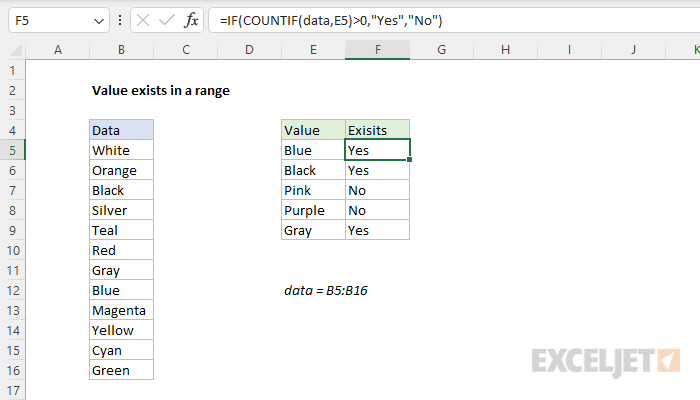
Summary
To test if a value exists in a range of cells, you can use a simple formula based on the COUNTIF function and the IF function. In the example shown, the formula in F5, copied down, is:
where data is the named range B5:B16. As the formula is copied down it returns «Yes» if the value in column E exists in B5:B16 and «No» if not.
Generic formula
Explanation
In this example, the goal is to use a formula to check if a specific value exists in a range. The easiest way to do this is to use the COUNTIF function to count occurences of a value in a range, then use the count to create a final result.
COUNTIF function
The COUNTIF function counts cells that meet supplied criteria. The generic syntax looks like this:
Range is the range of cells to test, and criteria is a condition that should be tested. COUNTIF returns the number of cells in range that meet the condition defined by criteria. If no cells meet criteria, COUNTIF returns zero. In the example shown, we can use COUNTIF to count the values we are looking for like this
Once the named range data (B5:B16) and cell E5 have been evaluated, we have:
COUNTIF returns 1 because «Blue» occurs in the range B5:B16 once. Next, we use the greater than operator (>) to run a simple test to force a TRUE or FALSE result:
By itself, the formula above will return TRUE or FALSE. The last part of the problem is to return a «Yes» or «No» result. To handle this, we nest the formula above into the IF function like this:
This is the formula shown in the worksheet above. As the formula is copied down, COUNTIF returns a count of the value in column E. If the count is greater than zero, the IF function returns «Yes». If the count is zero, IF returns «No».
Slightly abbreviated
It is possible to shorten this formula slightly and get the same result like this:
Here, we have remove the «>0» test. Instead, we simply return the count to IF as the logical_test. This works because Excel will treat any non-zero number as TRUE when the number is evaluated as a Boolean.
Testing for a partial match
To test a range to see if it contains a substring (a partial match), you can add a wildcard to the formula. For example, if you have a value to look for in cell C1, and you want to check the range A1:A100 for partial matches, you can configure COUNTIF to look for the value in C1 anywhere in a cell by concatenating asterisks on both sides:
The asterisk (*) is a wildcard for one or more characters. By concatenating asterisks before and after the value in C1, the formula will count the text in C1 anywhere it appears in each cell of the range. To return «Yes» or «No», nest the formula inside the IF function as above.
An alternative formula using MATCH
As an alternative, you can use a formula that uses the MATCH function with the ISNUMBER function instead of COUNTIF:
The MATCH function returns the position of a match (as a number) if found, and #N/A if not found. By wrapping MATCH inside ISNUMBER, the final result will be TRUE when MATCH finds a match and FALSE when MATCH returns #N/A.
Источник
Finding of the value in the column and the row of the Excel table
We have the table in which the sales volumes of certain products are recorded in different months. It is necessary to find the data in the table, and the search criteria will be the headings of rows and columns. But the search must be performed separately by the range of the row or column. That is, only one of the criteria will be used. Therefore, you can`t apply the INDEX function here, but you need a special formula.
Finding values in the Excel table
To solve this problem, let us illustrate the example in the schematic table that corresponds to the conditions are described above.
The sheet with the table to search for values vertically and horizontally:
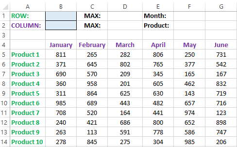
Above this table we can see the row with results. In the cell B1 we introduce the criterion for the search query, that is, the column header or the ROW name. And in the cell D1, to a search formula should return to the result of the calculation of the corresponding value. Then the second formula will work in the cell F1. She will already use the values of the cells B1 and D1 as the criteria for searching of the corresponding month.
Search of the value in the Excel ROW
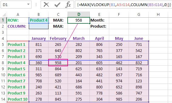
Now we are learning, in what maximum volume and in what month has been the maximum sale of the Product 4.
To search by columns:
- In the cell B1 you need to enter the value of the Product 4 — the name of the row, that will act as the criterion.
- In the cell D1 you need to enter the following:
- To confirm after entering the formula, you need to press the CTRL + SHIFT + Enter hotkey combination, because she must be executed in the array. If everything is done correctly, the curly braces will appear in the formula ROW.

- In the cell F1 you need to enter the second:
- For confirmation, to press the key combination CTRL + SHIFT + Enter again.
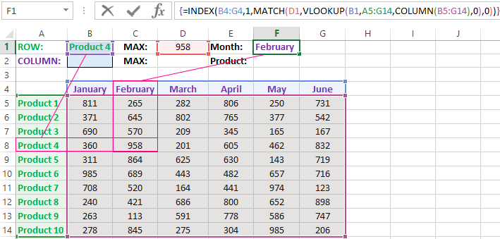
So we have found, in what month and what was the largest sale of the Product 4 for two quarters.
The principle of the formula for finding the value in the Excel ROW:
In the first argument of the VLOOKUP function (Vertical Look Up), indicates to the reference to the cell, where the search criterion is located. In the second argument indicates to the range of the cells for viewing during in the process of searching.
In the third argument of the VLOOKUP function should be indicated the number of the column from which you should to take the value against of the row named the Item 4. But since we do not previously know this number, we use the COLUMN function for creating the array of column numbers for the range B4:G15.
This allows the VLOOKUP function to collect the whole array of values. As a result, all relevant values are stored in memory for each column in the row Product 4 (namely: 360; 958; 201; 605; 462; 832). After that, the MAX function will only take the maximum number from this array and return it as the value for the cell D1, as the result of calculating.
As you can see, the construction of the formula is simple and concise. On its basis, it is possible in a similar way to find other indicators for a certain product. For example, the minimum or an average value of sales volume you need to find using for this purpose MIN or AVERAGE functions. Nothing hinders you from applying this skeleton of the formula to apply with more complex functions for implementation the most comfortable analysis of the sales report.
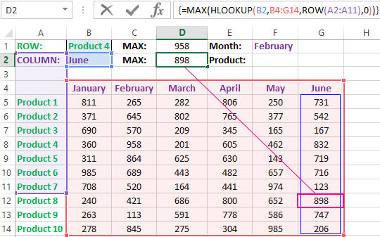
How can I get to the column headings from a single cell value?
For example, how effectively we displayed the month with the maximum sale, using of the second. It’s not difficult to notice that in the second formula we used the skeleton of the first formula without the MAX function. The main structure of the function is: VLOOKUP. We replaced the MAX on the MATCH, which in the first argument uses the value obtained by the previous formula. It acts as the criterion for searching for the month now.
And as a result, the MATCH function returns the column number 2, where the maximum value of the sales volume for the product is located for the product 4. After that, the INDEX function is included in the work. This function returns the value by the number of terms and column from the range specified in its arguments. Because the we have the number of column 2, and the row number in the range where the names of months are stored in any cases will be the value 1. Then we have the INDEX function to get the corresponding value from the range of B4:G4 — February (the second month).
Search the value in the Excel column
The second version of the task will be searching in the table with using the month name as the criterion. In such cases, we have to change the skeleton of our formula: the VLOOKUP function is replaced by the HLOOKUP (Horizontal Look Up) one, and the COLUMN function is replaced by the row one.
This will allow us to know what volume and what of the product the maximum sale was in a certain month.
To find what kind of the product had the maximum sales in a certain month, you should:
- In the cell B2 to enter the name of the month June — this value will be used as the search criterion.
- In the cell D2, you should to enter the formula:
- To confirm after entering the formula you need to press the combination of keys CTRL + SHIFT + Enter, as this formula will be executed in the array. And the curly braces will appear in the function ROW.
- In the cell F1, you need to enter the second:
- You need to click CTRL + SHIFT + Enter for confirmation again.
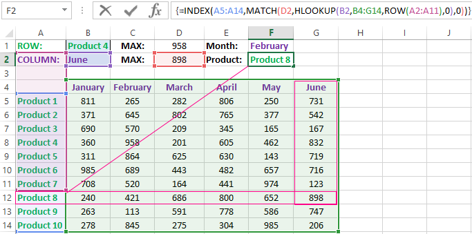
The principle of the formula for finding the value in the Excel column
In the first argument of the HLOOKUP function, we indicate to the reference by the cell with the criterion for the search. In the second argument specifies the reference to the table argument being scanned. The third argument is generated by the ROW function, what creates in the array of ROW numbers of 10 elements in memory. So there are 10 rows in the table section.
Further the HLOOKUP function, alternately using to each number of the row, creates the array of corresponding sales values from the table for the certain month (June). Further, the MAX function is left only to select the maximum value from this array.
Then just a little modifying to the first formula by using the INDEX and MATCH functions, we created the second function to display the names of the table rows according to the cell value. The names of the corresponding rows (products) we output in F2.
ATTENTION! When using the formula skeleton for other tasks, you need always to pay attention to the second and the third argument of the search HLOOKUP function. The number of covered rows in the range is specified in the argument, must match with the number of rows in the table. And also the numbering should begin with the second ROW!
Indeed, the content of the range generally we don’t care — we just need the row counter. That is, you need to change the arguments to: ROW(B2:B11) or ROW(C2:C11) — this does not affect in the quality of the formula. The main thing is that — there are 10 rows in these ranges, as well as in the table. And the numbering starts from the second row!
Источник
Transcript
In this lesson, we’ll look at how to find things in Excel.
Let’s take a look.
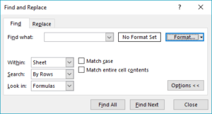
To find a value in Excel, use the Find and Replace dialog box. You can access this dialog using the keyboard shortcut control-F, or, by using the Find and Select menu at the far right of the Home tab on the ribbon.
Let’s try looking for the name Ann. Nothing happens until we click the Find Next button. Then, each time we click, Excel finds another match.
Note that Excel finds other names that contain Ann as well—Annie, Ann, Danny, and then Hannah. If we continue clicking Find Next, Excel will eventually return to the first match.
By default, Excel searches left to right, first through rows, then columns. You can hold down the shift key when you press «Find Next» to move backwards.
Now let’s review the Find options.
The first option allows you to restrict the search to the current worksheet, or expand it to include the entire workbook. If we select workbook, Excel will now find matches on Sheet 2.
The «search» option determines the order that Excel looks through cells. The default is «By Rows.» If we switch to «By Columns,» Excel will find all matches in one column before moving on to the next column.
There is also an option to search Formulas, Values, and Comments. We’ll look at these in a future lesson.
If we enable «Match case,» Excel treats case as important and only finds values that begin with a capital A.
If we enable «Match entire cell contents,» Excel will only find cells where the value is exactly Ann. This is a good way to find only the name Ann.
With the Find dialog closed, you can still find things with the keyboard shortcut Shift F4. Excel will use the current Find settings and select the next match.
Finally, it’s important to understand that if you have more than one cell selected, Excel will search only in the current selection. For example, if we select just a subset of our table, Excel will only search in that selection.
However, if you switch «Within» to «Workbook,» Excel will drop the current selection and search all cells. At this point, you can switch back to Worksheet to search only the current worksheet.
Many times as a developer you might need to find a match to a particular value in a range or sheet, and this is often done using a loop. However, VBA provides a much more efficient way of accomplishing this using the Find method. In this article we’ll have a look at how to use the Range.Find Method in your VBA code. Here is the syntax of the method:
expression.Find (What , After , LookIn , LookAt , SearchOrder , SearchDirection , MatchCase , MatchByte , SearchFormat )
where:
What: The data to search for. It can be a string or any of the Microsoft Excel data types (the only required parameter, rest are all optional)
After: The cell after which you want the search to begin. It is a single cell which is excluded from search. Default value is the upper-left corner of the range specified.
LookIn: Look in formulas, values or notes using constants xlFormulas, xlValues, or xlNotes respectively.
LookAt: Look at a whole value of a cell or part of it (xlWhole or xlPart)
SearchOrder: Search can be by rows or columns (xlByRows or xlByColumns)
SearchDirection: Direction of search (xlNext, xlPrevious)
MatchCase: Case sensitive or the default insensitive (True or False)
MatchByte: Used only for double byte languages (True or False)
SearchFormat: Search by format (True or False)
All these parameters correspond to the find dialog box options in Excel.
Return Value: A Range object that represents the first cell where the data was found. (Nothing if match is not found).
Let us look at some examples on how to implement this. In all the examples below, we will be using the table below to perform the search on.

Example 1: A basic search
In this example, we will look for a value in the name column.
Dim foundRng As Range Set foundRng = Range("D3:D19").Find("Andrea") MsgBox foundRng.AddressThe rest of the parameters are optional. If you don’t use them then Find will use the existing settings. We’ll see more about this shortly.
The output of this code will be the first occurrence of the search string in the specified range.
If the search item is not found then Find returns an object set to Nothing. And an error will be thrown if you try to perform any operation on this (on foundRng in the above example)
So, it is always advisable to check whether the value is found before performing any further operations.
Dim foundRng As Range Set foundRng = Range("D3:D19").Find("Andrea") If foundRng Is Nothing Then MsgBox "Value not found" Else MsgBox foundRng.Address End IfLet us know have a look at the optional parameters. To keep it simple, we will exclude the above error handling in the subsequent examples.
Example 2: Using after
Set foundRng = Range("D3:D19").Find("Andrea", Range("D6"&amp;amp;amp;amp;amp;amp;lt;span data-mce-type="bookmark" style="display: inline-block; width: 0px; overflow: hidden; line-height: 0;" class="mce_SELRES_start"&amp;amp;amp;amp;amp;amp;gt;&amp;amp;amp;amp;amp;amp;lt;/span&amp;amp;amp;amp;amp;amp;gt;)) MsgBox foundRng.AddressOR
Set foundRng = Range("D3:D19").Find("Andrea", After:=Range("D6")) MsgBox foundRng.AddressThe highlighted cell will be searched for
Example 3: Using LookIn
Before seeing an example, here are few things to note with LookIn
- Text is considered as a value as well as a formula
- xlNotes is same as xlComments
- Once you set the value of LookIn all subsequent searches will use this setting of LookIn (using VBA or Excel)
'Look in values Set foundRng = Range("A3:H19").Find("F4", , xlValues) MsgBox foundRng.Address 'Output --&amp;amp;amp;amp;amp;amp;gt; $B$4 'Look in values and formula Set foundRng = Range("A3:H19").Find("F4", LookIn:=xlFormulas) MsgBox foundRng.Address 'Output --&amp;amp;amp;amp;amp;amp;gt; $B$4 'Look in values and formula (as previous setting is preserved) Set foundRng = Range("H3:H19").Find("F4") MsgBox foundRng.Address 'Output --&amp;amp;amp;amp;amp;amp;gt; $H$4 'Look in comments Set foundRng = Range("A3:H19").Find("F4", , xlNotes) MsgBox foundRng.Address 'Output --&amp;amp;amp;amp;amp;amp;gt; $D$4
Example 4: Using LookAt
'Match only a part of a cell Set foundRng = Range("A3:H19").Find("John", , xlValues, xlPart) MsgBox foundRng.Address 'Output --&amp;amp;amp;amp;amp;amp;gt; $D$8 'Match entire cell contents Set foundRng = Range("A3:H19").Find("John", LookAt:=xlWhole) MsgBox foundRng.Address 'Output --&amp;amp;amp;amp;amp;amp;gt; $D$9LookAt setting too is preserved for subsequent searches.
Example 5: Using SearchOrder
'Searches by rows Set foundRng = Range("A3:H19").Find("Sa", , , xlPart, xlRows) MsgBox foundRng.Address 'Output --&amp;amp;amp;amp;amp;amp;gt; $G$4 'Searches by columns Set foundRng = Range("A3:H19").Find("Sa", SearchOrder:=xlColumns) MsgBox foundRng.Address 'Output --&amp;amp;amp;amp;amp;amp;gt; $F$5SearchOrder setting is preserved for subsequent searches.
Example 6: Using SearchDirection
'Searches from the bottom Set foundRng = Range("A3:H19").Find("Alexander", , , , , xlPrevious) MsgBox foundRng.Address 'Output --&amp;amp;amp;amp;amp;amp;gt; $D$18 'Searches from the top Set foundRng = Range("A3:H19").Find("Alexander", SearchDirection:=xlNext) MsgBox foundRng.Address 'Output --&amp;amp;amp;amp;amp;amp;gt; $D$11
Example 7: Using MatchCase
'Match Case Set foundRng = Range("A3:H19").Find("Sa", , , , xlRows, , True) MsgBox foundRng.Address 'Output --&amp;amp;amp;amp;amp;amp;gt; $F$5 'Ignore case Set foundRng = Range("A3:H19").Find("Sa", MatchCase:=False) MsgBox foundRng.Address 'Output --&amp;amp;amp;amp;amp;amp;gt; $G$4
Example 8: Using SearchFormat
When you search for a format it is important to note that the format settings stick until you change them. So, before you use SearchFormat, it is a good practice to always clear any previous formats that have been set.
'Clear any previous format set Application.FindFormat.Clear 'Set the format for find operation Application.FindFormat.Interior.Color = 14348258 'Match format Set foundRng = Range("A3:H19").Find("SA", MatchCase:=True, SearchFormat:=True) MsgBox foundRng.Address 'Output --&amp;amp;amp;amp;amp;amp;gt; $G$15 'Search without matching the format Set foundRng = Range("A3:H19").Find("SA", MatchCase:=True, SearchFormat:=False) MsgBox foundRng.Address 'Output --&amp;amp;amp;amp;amp;amp;gt; $G$4 'Search only for cells of a particular format Set foundRng = Range("B3:H19").Find("*", MatchCase:=True, SearchFormat:=True) MsgBox foundRng.Address 'Output --&amp;amp;amp;amp;amp;amp;gt; $B$3
Example 9: FindNext and FindPrevious
In all the previous examples, we have been looking for just the first occurrence of the search criteria. If you want to find multiple occurrences, we use the FindNext and FindPrevious methods. Both of these need a reference to the last cell found, so that the search continues after that cell. If this argument is dropped, it will keep returning the first occurrence.
'First occurrence Set foundRng = Range("A3:H19").Find("Ms") MsgBox foundRng.Address 'Output --&amp;amp;amp;amp;amp;amp;gt; $C$5 'Find the next occurrence Set foundRng = Range("A3:H19").FindNext(foundRng) MsgBox foundRng.Address 'Output --&amp;amp;amp;amp;amp;amp;gt; $C$10 'Find the previous occurrence again Set foundRng = Range("A3:H19").FindPrevious(foundRng) MsgBox foundRng.Address 'Output --&amp;amp;amp;amp;amp;amp;gt; $C$5
If you are looking to find or list all files and directories in a folder / sub-folder, you can refer to the articles below:
Find and List all Files and Folders in a Directory
Excel VBA, Find and List All Files in a Directory and its Subdirectories
For using other methods in addition to Find, please see:
Check if Cell Contains Values in Excel


We have the table in which the sales volumes of certain products are recorded in different months. It is necessary to find the data in the table, and the search criteria will be the headings of rows and columns. But the search must be performed separately by the range of the row or column. That is, only one of the criteria will be used. Therefore, you can`t apply the INDEX function here, but you need a special formula.
Finding values in the Excel table
To solve this problem, let us illustrate the example in the schematic table that corresponds to the conditions are described above.
The sheet with the table to search for values vertically and horizontally:
Above this table we can see the row with results. In the cell B1 we introduce the criterion for the search query, that is, the column header or the ROW name. And in the cell D1, to a search formula should return to the result of the calculation of the corresponding value. Then the second formula will work in the cell F1. She will already use the values of the cells B1 and D1 as the criteria for searching of the corresponding month.
Search of the value in the Excel ROW
Now we are learning, in what maximum volume and in what month has been the maximum sale of the Product 4.
To search by columns:
- In the cell B1 you need to enter the value of the Product 4 — the name of the row, that will act as the criterion.
- In the cell D1 you need to enter the following:
- To confirm after entering the formula, you need to press the CTRL + SHIFT + Enter hotkey combination, because she must be executed in the array. If everything is done correctly, the curly braces will appear in the formula ROW.
- In the cell F1 you need to enter the second:
- For confirmation, to press the key combination CTRL + SHIFT + Enter again.
So we have found, in what month and what was the largest sale of the Product 4 for two quarters.
The principle of the formula for finding the value in the Excel ROW:
In the first argument of the VLOOKUP function (Vertical Look Up), indicates to the reference to the cell, where the search criterion is located. In the second argument indicates to the range of the cells for viewing during in the process of searching.
In the third argument of the VLOOKUP function should be indicated the number of the column from which you should to take the value against of the row named the Item 4. But since we do not previously know this number, we use the COLUMN function for creating the array of column numbers for the range B4:G15.
This allows the VLOOKUP function to collect the whole array of values. As a result, all relevant values are stored in memory for each column in the row Product 4 (namely: 360; 958; 201; 605; 462; 832). After that, the MAX function will only take the maximum number from this array and return it as the value for the cell D1, as the result of calculating.
As you can see, the construction of the formula is simple and concise. On its basis, it is possible in a similar way to find other indicators for a certain product. For example, the minimum or an average value of sales volume you need to find using for this purpose MIN or AVERAGE functions. Nothing hinders you from applying this skeleton of the formula to apply with more complex functions for implementation the most comfortable analysis of the sales report.
How can I get to the column headings from a single cell value?
For example, how effectively we displayed the month with the maximum sale, using of the second. It’s not difficult to notice that in the second formula we used the skeleton of the first formula without the MAX function. The main structure of the function is: VLOOKUP. We replaced the MAX on the MATCH, which in the first argument uses the value obtained by the previous formula. It acts as the criterion for searching for the month now.
And as a result, the MATCH function returns the column number 2, where the maximum value of the sales volume for the product is located for the product 4. After that, the INDEX function is included in the work. This function returns the value by the number of terms and column from the range specified in its arguments. Because the we have the number of column 2, and the row number in the range where the names of months are stored in any cases will be the value 1. Then we have the INDEX function to get the corresponding value from the range of B4:G4 — February (the second month).
Search the value in the Excel column
The second version of the task will be searching in the table with using the month name as the criterion. In such cases, we have to change the skeleton of our formula: the VLOOKUP function is replaced by the HLOOKUP (Horizontal Look Up) one, and the COLUMN function is replaced by the row one.
This will allow us to know what volume and what of the product the maximum sale was in a certain month.
To find what kind of the product had the maximum sales in a certain month, you should:
- In the cell B2 to enter the name of the month June — this value will be used as the search criterion.
- In the cell D2, you should to enter the formula:
- To confirm after entering the formula you need to press the combination of keys CTRL + SHIFT + Enter, as this formula will be executed in the array. And the curly braces will appear in the function ROW.
- In the cell F1, you need to enter the second:
- You need to click CTRL + SHIFT + Enter for confirmation again.
The principle of the formula for finding the value in the Excel column
In the first argument of the HLOOKUP function, we indicate to the reference by the cell with the criterion for the search. In the second argument specifies the reference to the table argument being scanned. The third argument is generated by the ROW function, what creates in the array of ROW numbers of 10 elements in memory. So there are 10 rows in the table section.
Further the HLOOKUP function, alternately using to each number of the row, creates the array of corresponding sales values from the table for the certain month (June). Further, the MAX function is left only to select the maximum value from this array.
Then just a little modifying to the first formula by using the INDEX and MATCH functions, we created the second function to display the names of the table rows according to the cell value. The names of the corresponding rows (products) we output in F2.
ATTENTION! When using the formula skeleton for other tasks, you need always to pay attention to the second and the third argument of the search HLOOKUP function. The number of covered rows in the range is specified in the argument, must match with the number of rows in the table. And also the numbering should begin with the second ROW!
Download example search values in the columns and rows
Read also: The searching of the value in a range Excel table in columns and rows
Indeed, the content of the range generally we don’t care — we just need the row counter. That is, you need to change the arguments to: ROW(B2:B11) or ROW(C2:C11) — this does not affect in the quality of the formula. The main thing is that — there are 10 rows in these ranges, as well as in the table. And the numbering starts from the second row!