
Содержание
- Cell contains number
- Related functions
- Summary
- Generic formula
- Explanation
- FIND function
- SEQUENCE function
- Cell equals number?
- FIND, FINDB functions
- Description
- Syntax
- Remarks
- Examples
- Find or replace text and numbers on a worksheet
- Replace
- Check if Cell Contains Any Number – Excel & Google Sheets
- Cell Contains Any Number
- FIND a Number in a Cell
- COUNT the Number of Digits
- Test the Number Count
- Check if Cell Contains Specific Number
- Check if Cell Contains Any Number – Google Sheets
Cell contains number
Summary
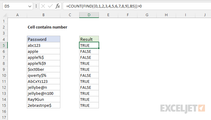
To test if a cell or text string contains a number, you can use the FIND function together with the COUNT function. The numbers to look for are supplied as an array constant. In the example the formula in D5 is:
As the formula is copied down, it returns TRUE if a value contains a number and FALSE if not. See below for an alternate formula based on the SEQUENCE function.
Generic formula
Explanation
In this example, the goal is to test the passwords in column B to see if they contain a number. This is a surprisingly tricky problem because Excel doesn’t have a function that will let you test for a number inside a text string directly. Note this is different from checking if a cell value is a number. You can easily perform that test with the ISNUMBER function. In this case, however, we to test if a cell value contains a number, which may occur anywhere. One solution is to use the FIND function with an array constant. In Excel 365, which supports dynamic array formulas, you can use a different formula based on the SEQUENCE function. Both approaches are explained below.
FIND function
The FIND function is designed to look inside a text string for a specific substring. If FIND finds the substring, it returns a position of the substring in the text as a number. If the substring is not found, FIND returns a #VALUE error. For example:
We can use this same idea to check for numbers as well:
The challenge in this case is that we need to check the values in column B for ten different numbers, 0-9. One way to do that is to supply these numbers as the array constant <0,1,2,3,4,5,6,7,8,9>. This is the approach taken in the formula in cell D5:
Inside the COUNT function, the FIND function is configured to look for all ten numbers in cell B5:
Because we are giving FIND ten values to look for, it returns an array with 10 results. In other words, FIND checks the text in B5 for each number and returns all results at once:
Unless you look at arrays often, this may look pretty cryptic. Here is the translation: The number 1 was found at position 4, the number 2 was found at position 5, and the number 3 was found at position 6. All other numbers were not found and returned #VALUE errors.
We are very close now to a final formula. We simply need to tally up results. To do this, we nest the FIND formula above inside the COUNT function like this:
FIND returns the array of results directly to COUNT, which counts the numbers in the array. COUNT only counts numeric values, and ignores errors. This means COUNT will return a number greater than zero if there are any numbers in the value being tested. In the case of cell B5, COUNT returns 3.
The last step is to check the result from COUNT and force a TRUE or FALSE result. We do this by adding «>0» to the end of formula:
Now the formula will return TRUE or FALSE. To display a custom result, you can use the IF function:
The original formula is now nested inside IF as the logical_test argument. This formula will return «Yes» if B5 contains a number and «No» if not.
SEQUENCE function
In Excel 365, which offers dynamic array formulas, we can take a different approach to this problem.
This isn’t necessarily a better approach, just a different way to solve the same problem. At the core, this formula uses the MID function together with the SEQUENCE function to split the text in cell B5 into an array:
Working from the inside out, the LEN function returns the length of the text in cell B5:
This number is returned to the SEQUENCE function as the rows argument, and SEQUENCE returns an array of numbers, 1-6:
This array is returned to the MID function as the start_num argument, and, with num_chars set to 1, the MID function returns an array that contains the characters in cell B5:
We can now simplify the original formula to:
We use the double-negative (—) to get Excel to try and coerce the values in the array into numbers. The result looks like this:
The math operation created by the double negative (—) returns an actual number when successful and a #VALUE! error when the operation fails. The COUNT function counts the numbers, ignoring any errors, and returns 3. As above, we check the final count with «>0», and the result for cell B5 is TRUE.
Note: as you might guess, you can easily adapt this formula to count numbers in a text string.
Cell equals number?
Note that the formulas above are too complex if you only want to test if a cell equals a number. In that case, you can simply use the ISNUMBER function like this:
Источник
FIND, FINDB functions
This article describes the formula syntax and usage of the FIND and FINDB functions in Microsoft Excel.
Description
FIND and FINDB locate one text string within a second text string, and return the number of the starting position of the first text string from the first character of the second text string.
These functions may not be available in all languages.
FIND is intended for use with languages that use the single-byte character set (SBCS), whereas FINDB is intended for use with languages that use the double-byte character set (DBCS). The default language setting on your computer affects the return value in the following way:
FIND always counts each character, whether single-byte or double-byte, as 1, no matter what the default language setting is.
FINDB counts each double-byte character as 2 when you have enabled the editing of a language that supports DBCS and then set it as the default language. Otherwise, FINDB counts each character as 1.
The languages that support DBCS include Japanese, Chinese (Simplified), Chinese (Traditional), and Korean.
Syntax
FIND(find_text, within_text, [start_num])
FINDB(find_text, within_text, [start_num])
The FIND and FINDB function syntax has the following arguments:
Find_text Required. The text you want to find.
Within_text Required. The text containing the text you want to find.
Start_num Optional. Specifies the character at which to start the search. The first character in within_text is character number 1. If you omit start_num, it is assumed to be 1.
FIND and FINDB are case sensitive and don’t allow wildcard characters. If you don’t want to do a case sensitive search or use wildcard characters, you can use SEARCH and SEARCHB.
If find_text is «» (empty text), FIND matches the first character in the search string (that is, the character numbered start_num or 1).
Find_text cannot contain any wildcard characters.
If find_text does not appear in within_text, FIND and FINDB return the #VALUE! error value.
If start_num is not greater than zero, FIND and FINDB return the #VALUE! error value.
If start_num is greater than the length of within_text, FIND and FINDB return the #VALUE! error value.
Use start_num to skip a specified number of characters. Using FIND as an example, suppose you are working with the text string «AYF0093.YoungMensApparel». To find the number of the first «Y» in the descriptive part of the text string, set start_num equal to 8 so that the serial-number portion of the text is not searched. FIND begins with character 8, finds find_text at the next character, and returns the number 9. FIND always returns the number of characters from the start of within_text, counting the characters you skip if start_num is greater than 1.
Examples
Copy the example data in the following table, and paste it in cell A1 of a new Excel worksheet. For formulas to show results, select them, press F2, and then press Enter. If you need to, you can adjust the column widths to see all the data.
Источник
Find or replace text and numbers on a worksheet

Use the Find and Replace features in Excel to search for something in your workbook, such as a particular number or text string. You can either locate the search item for reference, or you can replace it with something else. You can include wildcard characters such as question marks, tildes, and asterisks, or numbers in your search terms. You can search by rows and columns, search within comments or values, and search within worksheets or entire workbooks.
Tip: You can also use formulas to replace text. Check out the SUBSTITUTE function or REPLACE, REPLACEB functions to learn more.

To find something, press Ctrl+F, or go to Home > Editing > Find & Select > Find.
Note: In the following example, we’ve clicked the Options >> button to show the entire Find dialog. By default, it will display with Options hidden.

In the Find what: box, type the text or numbers you want to find, or click the arrow in the Find what: box, and then select a recent search item from the list.
Tips: You can use wildcard characters — question mark ( ?), asterisk ( *), tilde (
) — in your search criteria.
Use the question mark (?) to find any single character — for example, s?t finds «sat» and «set».
Use the asterisk (*) to find any number of characters — for example, s*d finds «sad» and «started».
) followed by ?, *, or
to find question marks, asterisks, or other tilde characters — for example, fy91
Click Find All or Find Next to run your search.
Tip: When you click Find All, every occurrence of the criteria that you are searching for will be listed, and clicking a specific occurrence in the list will select its cell. You can sort the results of a Find All search by clicking a column heading.
Click Options>> to further define your search if needed:
Within: To search for data in a worksheet or in an entire workbook, select Sheet or Workbook.
Search: You can choose to search either By Rows (default), or By Columns.
Look in: To search for data with specific details, in the box, click Formulas, Values, Notes, or Comments.
Note: Formulas, Values, Notes and Comments are only available on the Find tab; only Formulas are available on the Replace tab.
Match case — Check this if you want to search for case-sensitive data.
Match entire cell contents — Check this if you want to search for cells that contain just the characters that you typed in the Find what: box.
If you want to search for text or numbers with specific formatting, click Format, and then make your selections in the Find Format dialog box.
Tip: If you want to find cells that just match a specific format, you can delete any criteria in the Find what box, and then select a specific cell format as an example. Click the arrow next to Format, click Choose Format From Cell, and then click the cell that has the formatting that you want to search for.
Replace
To replace text or numbers, press Ctrl+H, or go to Home > Editing > Find & Select > Replace.
Note: In the following example, we’ve clicked the Options >> button to show the entire Find dialog. By default, it will display with Options hidden.

In the Find what: box, type the text or numbers you want to find, or click the arrow in the Find what: box, and then select a recent search item from the list.
Tips: You can use wildcard characters — question mark ( ?), asterisk ( *), tilde (
) — in your search criteria.
Use the question mark (?) to find any single character — for example, s?t finds «sat» and «set».
Use the asterisk (*) to find any number of characters — for example, s*d finds «sad» and «started».
) followed by ?, *, or
to find question marks, asterisks, or other tilde characters — for example, fy91
In the Replace with: box, enter the text or numbers you want to use to replace the search text.
Click Replace All or Replace.
Tip: When you click Replace All, every occurrence of the criteria that you are searching for will be replaced, while Replace will update one occurrence at a time.
Click Options>> to further define your search if needed:
Within: To search for data in a worksheet or in an entire workbook, select Sheet or Workbook.
Search: You can choose to search either By Rows (default), or By Columns.
Look in: To search for data with specific details, in the box, click Formulas, Values, Notes, or Comments.
Note: Formulas, Values, Notes and Comments are only available on the Find tab; only Formulas are available on the Replace tab.
Match case — Check this if you want to search for case-sensitive data.
Match entire cell contents — Check this if you want to search for cells that contain just the characters that you typed in the Find what: box.
If you want to search for text or numbers with specific formatting, click Format, and then make your selections in the Find Format dialog box.
Tip: If you want to find cells that just match a specific format, you can delete any criteria in the Find what box, and then select a specific cell format as an example. Click the arrow next to Format, click Choose Format From Cell, and then click the cell that has the formatting that you want to search for.
There are two distinct methods for finding or replacing text or numbers on the Mac. The first is to use the Find & Replace dialog. The second is to use the Search bar in the ribbon.
Источник
Check if Cell Contains Any Number – Excel & Google Sheets
Download the example workbook
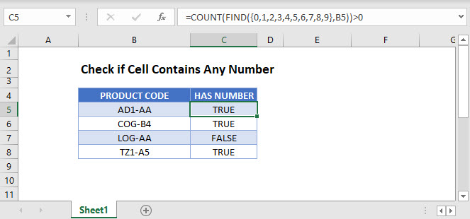
This tutorial demonstrates how to check if a cell contains any number in Excel and Google Sheets.
Cell Contains Any Number
In Excel, if a cell contains numbers and letters, the cell is considered a text cell. You can check if a text cell contains any number by using the COUNT and FIND Functions.
The formula above checks for the digits 0–9 in a cell and counts the number of discrete digits the cell contains. Then it returns TRUE if the count is positive or FALSE if it is zero.
Let’s step through each function below to understand this example.
FIND a Number in a Cell
First, we use the FIND Function. The FIND Function finds the position of a character within a text string.
In this example, we use an array of all numerical characters (digits 0–9) and find each one in the cell. Since our input is an array – in curly brackets <> – our output is also an array. The example above shows how the FIND Function is performed ten times on each cell (once for each numerical digit).
If the number is found, it’s position is output. Above you can see the number “1” is found in the 3rd position in the first row and “4” is found in the 6th position in the 2nd row.
If a number is not found, the #VALUE! Error is displayed.
Note: The FIND and SEARCH Functions return the same result when used to search for numbers. Either function can be used.
COUNT the Number of Digits
Next, we count the non-error outputs from the last step. The COUNT Function counts the number of numeric values found in the array, ignoring errors.
Test the Number Count
Finally, we need to test whether the result from the last step is greater than zero. The formula below returns TRUE for non-zero counts (where the target cell contains a number) and FALSE for any zero counts.
Combining these steps gives us our initial formula:
Check if Cell Contains Specific Number
To check if a cell contains a specific number, we can use the FIND or SEARCH Function.
In this example we use the FIND Function to check for the number 5 in column B. It returns the position of the number 5 in the cell if it is found and a VALUE error if “5” is not found.
Check if Cell Contains Any Number – Google Sheets
These formulas work the same in Google Sheets as in Excel. However, you need to press CTRL + SHIFT + ENTER for Google Sheets to recognize an array formula.
Alternatively, you could type “ArrayFormula” and put the formula in parentheses. Both methods produce the same result.
Источник
In this example, the goal is to test the passwords in column B to see if they contain a number. This is a surprisingly tricky problem because Excel doesn’t have a function that will let you test for a number inside a text string directly. Note this is different from checking if a cell value is a number. You can easily perform that test with the ISNUMBER function. In this case, however, we to test if a cell value contains a number, which may occur anywhere. One solution is to use the FIND function with an array constant. In Excel 365, which supports dynamic array formulas, you can use a different formula based on the SEQUENCE function. Both approaches are explained below.
FIND function
The FIND function is designed to look inside a text string for a specific substring. If FIND finds the substring, it returns a position of the substring in the text as a number. If the substring is not found, FIND returns a #VALUE error. For example:
=FIND("p","apple") // returns 2
=FIND("z","apple") // returns #VALUE!
We can use this same idea to check for numbers as well:
=FIND(3,"app637") // returns 5
=FIND(9,"app637") // returns #VALUE!
The challenge in this case is that we need to check the values in column B for ten different numbers, 0-9. One way to do that is to supply these numbers as the array constant {0,1,2,3,4,5,6,7,8,9}. This is the approach taken in the formula in cell D5:
=COUNT(FIND({0,1,2,3,4,5,6,7,8,9},B5))>0Inside the COUNT function, the FIND function is configured to look for all ten numbers in cell B5:
FIND({0,1,2,3,4,5,6,7,8,9},B5)Because we are giving FIND ten values to look for, it returns an array with 10 results. In other words, FIND checks the text in B5 for each number and returns all results at once:
{#VALUE!,4,5,6,#VALUE!,#VALUE!,#VALUE!,#VALUE!,#VALUE!,#VALUE!}Unless you look at arrays often, this may look pretty cryptic. Here is the translation: The number 1 was found at position 4, the number 2 was found at position 5, and the number 3 was found at position 6. All other numbers were not found and returned #VALUE errors.
We are very close now to a final formula. We simply need to tally up results. To do this, we nest the FIND formula above inside the COUNT function like this:
=COUNT(FIND({0,1,2,3,4,5,6,7,8,9},B5))FIND returns the array of results directly to COUNT, which counts the numbers in the array. COUNT only counts numeric values, and ignores errors. This means COUNT will return a number greater than zero if there are any numbers in the value being tested. In the case of cell B5, COUNT returns 3.
The last step is to check the result from COUNT and force a TRUE or FALSE result. We do this by adding «>0» to the end of formula:
=COUNT(FIND({0,1,2,3,4,5,6,7,8,9},B5))>0Now the formula will return TRUE or FALSE. To display a custom result, you can use the IF function:
=IF(COUNT(FIND({0,1,2,3,4,5,6,7,8,9},B5))>0, "Yes", "No")
The original formula is now nested inside IF as the logical_test argument. This formula will return «Yes» if B5 contains a number and «No» if not.
SEQUENCE function
In Excel 365, which offers dynamic array formulas, we can take a different approach to this problem.
=COUNT(--MID(B5,SEQUENCE(LEN(B5)),1))>0This isn’t necessarily a better approach, just a different way to solve the same problem. At the core, this formula uses the MID function together with the SEQUENCE function to split the text in cell B5 into an array:
MID(B5,SEQUENCE(LEN(B5)),1)Working from the inside out, the LEN function returns the length of the text in cell B5:
LEN(B5) // returns 6This number is returned to the SEQUENCE function as the rows argument, and SEQUENCE returns an array of numbers, 1-6:
=SEQUENCE(LEN(B5))
=SEQUENCE(6)
={1;2;3;4;5;6}
This array is returned to the MID function as the start_num argument, and, with num_chars set to 1, the MID function returns an array that contains the characters in cell B5:
=MID(B5,{1;2;3;4;5;6},1)
={"a";"b";"c";"1";"2";"3"}
We can now simplify the original formula to:
=COUNT(--{"a";"b";"c";"1";"2";"3"})>0We use the double-negative (—) to get Excel to try and coerce the values in the array into numbers. The result looks like this:
=COUNT({#VALUE!;#VALUE!;#VALUE!;1;2;3})>0The math operation created by the double negative (—) returns an actual number when successful and a #VALUE! error when the operation fails. The COUNT function counts the numbers, ignoring any errors, and returns 3. As above, we check the final count with «>0», and the result for cell B5 is TRUE.
Note: as you might guess, you can easily adapt this formula to count numbers in a text string.
Cell equals number?
Note that the formulas above are too complex if you only want to test if a cell equals a number. In that case, you can simply use the ISNUMBER function like this:
=ISNUMBER(A1)
This tutorial demonstrates how to check if a cell contains any number in Excel and Google Sheets.
Cell Contains Any Number
In Excel, if a cell contains numbers and letters, the cell is considered a text cell. You can check if a text cell contains any number by using the COUNT and FIND Functions.
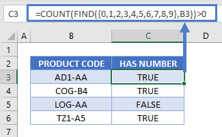
=COUNT(FIND({0,1,2,3,4,5,6,7,8,9},B3))>0
The formula above checks for the digits 0–9 in a cell and counts the number of discrete digits the cell contains. Then it returns TRUE if the count is positive or FALSE if it is zero.
Let’s step through each function below to understand this example.
FIND a Number in a Cell
First, we use the FIND Function. The FIND Function finds the position of a character within a text string.
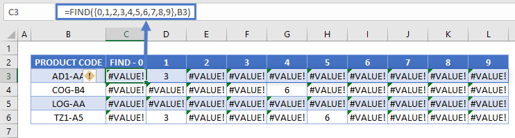
=FIND({0,1,2,3,4,5,6,7,8,9},B3)
In this example, we use an array of all numerical characters (digits 0–9) and find each one in the cell. Since our input is an array – in curly brackets {} – our output is also an array. The example above shows how the FIND Function is performed ten times on each cell (once for each numerical digit).
If the number is found, it’s position is output. Above you can see the number “1” is found in the 3rd position in the first row and “4” is found in the 6th position in the 2nd row.
If a number is not found, the #VALUE! Error is displayed.
Note: The FIND and SEARCH Functions return the same result when used to search for numbers. Either function can be used.
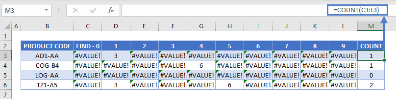
COUNT the Number of Digits
Next, we count the non-error outputs from the last step. The COUNT Function counts the number of numeric values found in the array, ignoring errors.
=COUNT(C3:L3)
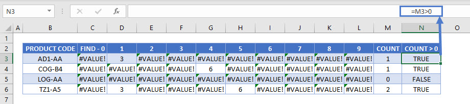
Test the Number Count
Finally, we need to test whether the result from the last step is greater than zero. The formula below returns TRUE for non-zero counts (where the target cell contains a number) and FALSE for any zero counts.
=M3>0
Combining these steps gives us our initial formula:
=COUNT(FIND({0,1,2,3,4,5,6,7,8,9},B3))>0
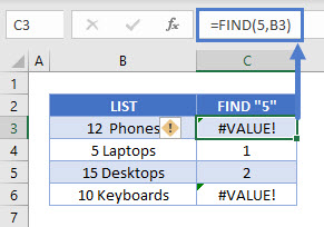
Check if Cell Contains Specific Number
To check if a cell contains a specific number, we can use the FIND or SEARCH Function.
=FIND(5,B3)
In this example we use the FIND Function to check for the number 5 in column B. It returns the position of the number 5 in the cell if it is found and a VALUE error if “5” is not found.
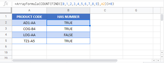
Check if Cell Contains Any Number – Google Sheets
These formulas work the same in Google Sheets as in Excel. However, you need to press CTRL + SHIFT + ENTER for Google Sheets to recognize an array formula.
Alternatively, you could type “ArrayFormula” and put the formula in parentheses. Both methods produce the same result.
Use the Find and Replace features in Excel to search for something in your workbook, such as a particular number or text string. You can either locate the search item for reference, or you can replace it with something else. You can include wildcard characters such as question marks, tildes, and asterisks, or numbers in your search terms. You can search by rows and columns, search within comments or values, and search within worksheets or entire workbooks.
Find
To find something, press Ctrl+F, or go to Home > Editing > Find & Select > Find.
Note: In the following example, we’ve clicked the Options >> button to show the entire Find dialog. By default, it will display with Options hidden.
-
In the Find what: box, type the text or numbers you want to find, or click the arrow in the Find what: box, and then select a recent search item from the list.
Tips: You can use wildcard characters — question mark (?), asterisk (*), tilde (~) — in your search criteria.
-
Use the question mark (?) to find any single character — for example, s?t finds «sat» and «set».
-
Use the asterisk (*) to find any number of characters — for example, s*d finds «sad» and «started».
-
Use the tilde (~) followed by ?, *, or ~ to find question marks, asterisks, or other tilde characters — for example, fy91~? finds «fy91?».
-
-
Click Find All or Find Next to run your search.
Tip: When you click Find All, every occurrence of the criteria that you are searching for will be listed, and clicking a specific occurrence in the list will select its cell. You can sort the results of a Find All search by clicking a column heading.
-
Click Options>> to further define your search if needed:
-
Within: To search for data in a worksheet or in an entire workbook, select Sheet or Workbook.
-
Search: You can choose to search either By Rows (default), or By Columns.
-
Look in: To search for data with specific details, in the box, click Formulas, Values, Notes, or Comments.
Note: Formulas, Values, Notes and Comments are only available on the Find tab; only Formulas are available on the Replace tab.
-
Match case — Check this if you want to search for case-sensitive data.
-
Match entire cell contents — Check this if you want to search for cells that contain just the characters that you typed in the Find what: box.
-
-
If you want to search for text or numbers with specific formatting, click Format, and then make your selections in the Find Format dialog box.
Tip: If you want to find cells that just match a specific format, you can delete any criteria in the Find what box, and then select a specific cell format as an example. Click the arrow next to Format, click Choose Format From Cell, and then click the cell that has the formatting that you want to search for.
Replace
To replace text or numbers, press Ctrl+H, or go to Home > Editing > Find & Select > Replace.
Note: In the following example, we’ve clicked the Options >> button to show the entire Find dialog. By default, it will display with Options hidden.
-
In the Find what: box, type the text or numbers you want to find, or click the arrow in the Find what: box, and then select a recent search item from the list.
Tips: You can use wildcard characters — question mark (?), asterisk (*), tilde (~) — in your search criteria.
-
Use the question mark (?) to find any single character — for example, s?t finds «sat» and «set».
-
Use the asterisk (*) to find any number of characters — for example, s*d finds «sad» and «started».
-
Use the tilde (~) followed by ?, *, or ~ to find question marks, asterisks, or other tilde characters — for example, fy91~? finds «fy91?».
-
-
In the Replace with: box, enter the text or numbers you want to use to replace the search text.
-
Click Replace All or Replace.
Tip: When you click Replace All, every occurrence of the criteria that you are searching for will be replaced, while Replace will update one occurrence at a time.
-
Click Options>> to further define your search if needed:
-
Within: To search for data in a worksheet or in an entire workbook, select Sheet or Workbook.
-
Search: You can choose to search either By Rows (default), or By Columns.
-
Look in: To search for data with specific details, in the box, click Formulas, Values, Notes, or Comments.
Note: Formulas, Values, Notes and Comments are only available on the Find tab; only Formulas are available on the Replace tab.
-
Match case — Check this if you want to search for case-sensitive data.
-
Match entire cell contents — Check this if you want to search for cells that contain just the characters that you typed in the Find what: box.
-
-
If you want to search for text or numbers with specific formatting, click Format, and then make your selections in the Find Format dialog box.
Tip: If you want to find cells that just match a specific format, you can delete any criteria in the Find what box, and then select a specific cell format as an example. Click the arrow next to Format, click Choose Format From Cell, and then click the cell that has the formatting that you want to search for.
There are two distinct methods for finding or replacing text or numbers on the Mac. The first is to use the Find & Replace dialog. The second is to use the Search bar in the ribbon.
Find & Replace dialog
Search bar and options

-
Press Ctrl+F or go to Home > Find & Select > Find.
-
In Find what: type the text or numbers you want to find.
-
Select Find Next to run your search.
-
You can further define your search:
-
Within: To search for data in a worksheet or in an entire workbook, select Sheet or Workbook.
-
Search: You can choose to search either By Rows (default), or By Columns.
-
Look in: To search for data with specific details, in the box, click Formulas, Values, Notes, or Comments.
-
Match case — Check this if you want to search for case-sensitive data.
-
Match entire cell contents — Check this if you want to search for cells that contain just the characters that you typed in the Find what: box.
-
Tips: You can use wildcard characters — question mark (?), asterisk (*), tilde (~) — in your search criteria.
-
Use the question mark (?) to find any single character — for example, s?t finds «sat» and «set».
-
Use the asterisk (*) to find any number of characters — for example, s*d finds «sad» and «started».
-
Use the tilde (~) followed by ?, *, or ~ to find question marks, asterisks, or other tilde characters — for example, fy91~? finds «fy91?».

-
Press Ctrl+F or go to Home > Find & Select > Find.
-
In Find what: type the text or numbers you want to find.
-
Select Find All to run your search for all occurrences.

Note: The dialog box expands to show a list of all the cells that contain the search term, and the total number of cells in which it appears.
-
Select any item in the list to highlight the corresponding cell in your worksheet.
Note: You can edit the contents of the highlighted cell.

-
Press Ctrl+H or go to Home > Find & Select > Replace.
-
In Find what, type the text or numbers you want to find.
-
You can further define your search:
-
Within: To search for data in a worksheet or in an entire workbook, select Sheet or Workbook.
-
Search: You can choose to search either By Rows (default), or By Columns.
-
Match case — Check this if you want to search for case-sensitive data.
-
Match entire cell contents — Check this if you want to search for cells that contain just the characters that you typed in the Find what: box.
Tips: You can use wildcard characters — question mark (?), asterisk (*), tilde (~) — in your search criteria.
-
Use the question mark (?) to find any single character — for example, s?t finds «sat» and «set».
-
Use the asterisk (*) to find any number of characters — for example, s*d finds «sad» and «started».
-
Use the tilde (~) followed by ?, *, or ~ to find question marks, asterisks, or other tilde characters — for example, fy91~? finds «fy91?».
-
-
-
In the Replace with box, enter the text or numbers you want to use to replace the search text.
-
Select Replace or Replace All.
Tips:
-
When you select Replace All, every occurrence of the criteria that you are searching for is replaced.
-
When you select Replace, you can replace one instance at a time by selecting Next to highlight the next instance.
-
-
Select any cell to search the entire sheet or select a specific range of cells to search.
-
Press Command + F or select the magnifying glass to expand the Search bar and type the text or number you want to find in the search field.
Tips: You can use wildcard characters — question mark (?), asterisk (*), tilde (~) — in your search criteria.
-
Use the question mark (?) to find any single character — for example, s?t finds «sat» and «set».
-
Use the asterisk (*) to find any number of characters — for example, s*d finds «sad» and «started».
-
Use the tilde (~) followed by ?, *, or ~ to find question marks, asterisks, or other tilde characters — for example, fy91~? finds «fy91?».
-
-
Press return.
Notes:
-
To find the next instance of the item you are searching for, press return again or use the Find dialog box and select Find Next.
-
To specify additional search options, select the magnifying glass and select Search in Sheet or Search in Workbook. You can also select the Advanced option, which launches the Find dialog.
Tip: You can cancel a search in progress by pressing ESC.
-
Find
To find something, press Ctrl+F, or go to Home > Editing > Find & Select > Find.
Note: In the following example, we’ve clicked > Search Options to show the entire Find dialog. By default, it will display with Search Options hidden.

-
In the Find what: box, type the text or numbers you want to find.
Tips: You can use wildcard characters — question mark (?), asterisk (*), tilde (~) — in your search criteria.
-
Use the question mark (?) to find any single character — for example, s?t finds «sat» and «set».
-
Use the asterisk (*) to find any number of characters — for example, s*d finds «sad» and «started».
-
Use the tilde (~) followed by ?, *, or ~ to find question marks, asterisks, or other tilde characters — for example, fy91~? finds «fy91?».
-
-
Click Find Next or Find All to run your search.
Tip: When you click Find All, every occurrence of the criteria that you are searching for will be listed, and clicking a specific occurrence in the list will select its cell. You can sort the results of a Find All search by clicking a column heading.
-
Click > Search Options to further define your search if needed:
-
Within: To search for data within a certain selection, choose Selection. To search for data in a worksheet or in an entire workbook, select Sheet or Workbook.
-
Direction: You can choose to search either Down (default), or Up.
-
Match case — Check this if you want to search for case-sensitive data.
-
Match entire cell contents — Check this if you want to search for cells that contain just the characters that you typed in the Find what box.
-
Replace
To replace text or numbers, press Ctrl+H, or go to Home > Editing > Find & Select > Replace.
Note: In the following example, we’ve clicked > Search Options to show the entire Find dialog. By default, it will display with Search Options hidden.

-
In the Find what: box, type the text or numbers you want to find.
Tips: You can use wildcard characters — question mark (?), asterisk (*), tilde (~) — in your search criteria.
-
Use the question mark (?) to find any single character — for example, s?t finds «sat» and «set».
-
Use the asterisk (*) to find any number of characters — for example, s*d finds «sad» and «started».
-
Use the tilde (~) followed by ?, *, or ~ to find question marks, asterisks, or other tilde characters — for example, fy91~? finds «fy91?».
-
-
In the Replace with: box, enter the text or numbers you want to use to replace the search text.
-
Click Replace or Replace All.
Tip: When you click Replace All, every occurrence of the criteria that you are searching for will be replaced, while Replace will update one occurrence at a time.
-
Click > Search Options to further define your search if needed:
-
Within: To search for data within a certain selection, choose Selection. To search for data in a worksheet or in an entire workbook, select Sheet or Workbook.
-
Direction: You can choose to search either Down (default), or Up.
-
Match case — Check this if you want to search for case-sensitive data.
-
Match entire cell contents — Check this if you want to search for cells that contain just the characters that you typed in the Find what box.
-
Need more help?
You can always ask an expert in the Excel Tech Community or get support in the Answers community.
Recommended articles
Merge and unmerge cells
REPLACE, REPLACEB functions
Apply data validation to cells
Excel allows a user to check if a cell contains a number by using the COUNT and FIND functions. This step by step tutorial will assist all levels of Excel users in checking if a cell contains any number.
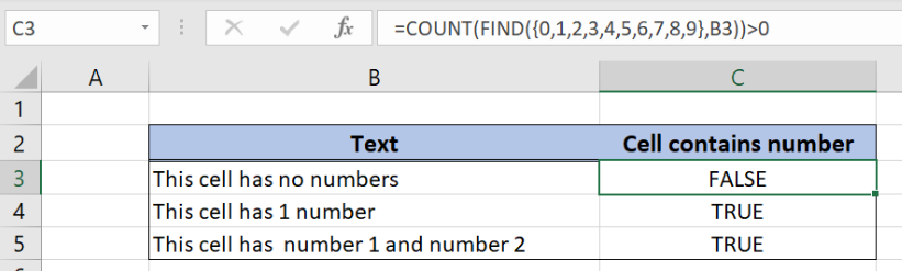 Figure 1. The result of the COUNT and FIND functions
Syntax of the FIND Formula
The generic formula for the FIND function is:
=FIND(find_text, within_text)
The parameters of the FIND function are:
- find_text – a text that we want to find in selected text or cell
- within_text – a text or cell where we want to find a text.
If a text is found, the FIND function returns a position of text in a cell. If it’s not found, the function returns #VALUE! error.
Syntax of the COUNT Formula
The generic formula for the COUNT function is:
=COUNT(value1, value2, ...., valueN)
The parameters of the COUNT function are:
- value1, value2, …, valueN – values that we want to count.
Setting up Our Data for the COUNT Function
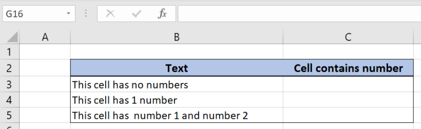 Figure 2. Data that we will use in the COUNT example
Let’s look at the structure of the data we will use. In column B we have texts, while in column C we want to return TRUE if the cell contains number and FALSE if not.
Check if cells contain a number
In our example, we want to check if texts from column B contain any number and return a result in column C.
The formula looks like:
=COUNT(FIND({0,1,2,3,4,5,6,7,8,9}, B3)) > 0
The parameter find_text of the FIND function is the array of numbers {0,1,2,3,4,5,6,7,8,9}. The within_text parameter is B3. When using the array, the FIND function will return a result for every element in the array. Let’s evaluate the formula and see the result:
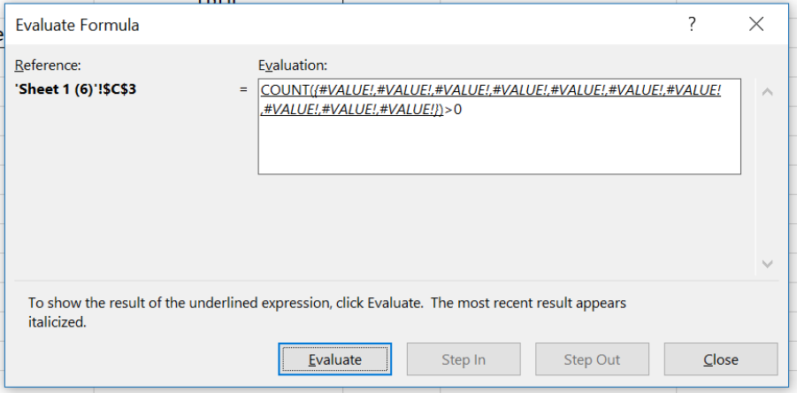 Figure 3. Evaluate the FIND function
The FIND function returned #VALUE! error for every element of the array, as there is no number in the array.
All of the results of the FIND function are parameters for COUNT function. As errors are not counted, the function returns 0. In the end, we check if the result of the COUNT is greater than 0. As it’s not, the result in the cell C3 is FALSE.
To apply the COUNT function, we need to follow these steps:
- Select cell C3 and click on it
- Insert the formula:
=COUNT(FIND({0,1,2,3,4,5,6,7,8,9}, B3)) > 0 - Press enter
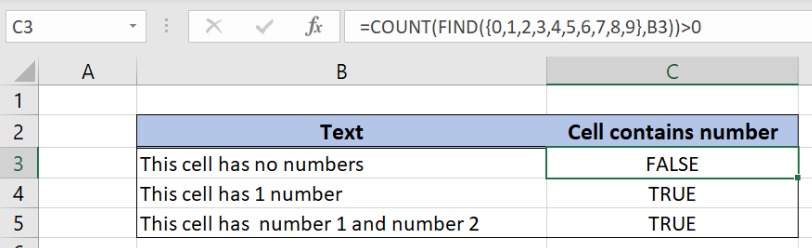 Figure 4. Using the COUNT and FIND functions to check if cells contain a number
Most of the time, the problem you will need to solve will be more complex than a simple application of a formula or function. If you want to save hours of research and frustration, try our live Excelchat service! Our Excel Experts are available 24/7 to answer any Excel question you may have. We guarantee a connection within 30 seconds and a customized solution within 20 minutes.