

Use the Find and Replace features in Excel to search for something in your workbook, such as a particular number or text string. You can either locate the search item for reference, or you can replace it with something else. You can include wildcard characters such as question marks, tildes, and asterisks, or numbers in your search terms. You can search by rows and columns, search within comments or values, and search within worksheets or entire workbooks.

Find
To find something, press Ctrl+F, or go to Home > Editing > Find & Select > Find.
Note: In the following example, we’ve clicked the Options >> button to show the entire Find dialog. By default, it will display with Options hidden.

-
In the Find what: box, type the text or numbers you want to find, or click the arrow in the Find what: box, and then select a recent search item from the list.
Tips: You can use wildcard characters — question mark (?), asterisk (*), tilde (~) — in your search criteria.
-
Use the question mark (?) to find any single character — for example, s?t finds «sat» and «set».
-
Use the asterisk (*) to find any number of characters — for example, s*d finds «sad» and «started».
-
Use the tilde (~) followed by ?, *, or ~ to find question marks, asterisks, or other tilde characters — for example, fy91~? finds «fy91?».
-
-
Click Find All or Find Next to run your search.
Tip: When you click Find All, every occurrence of the criteria that you are searching for will be listed, and clicking a specific occurrence in the list will select its cell. You can sort the results of a Find All search by clicking a column heading.
-
Click Options>> to further define your search if needed:
-
Within: To search for data in a worksheet or in an entire workbook, select Sheet or Workbook.
-
Search: You can choose to search either By Rows (default), or By Columns.
-
Look in: To search for data with specific details, in the box, click Formulas, Values, Notes, or Comments.
Note: Formulas, Values, Notes and Comments are only available on the Find tab; only Formulas are available on the Replace tab.
-
Match case — Check this if you want to search for case-sensitive data.
-
Match entire cell contents — Check this if you want to search for cells that contain just the characters that you typed in the Find what: box.
-
-
If you want to search for text or numbers with specific formatting, click Format, and then make your selections in the Find Format dialog box.
Tip: If you want to find cells that just match a specific format, you can delete any criteria in the Find what box, and then select a specific cell format as an example. Click the arrow next to Format, click Choose Format From Cell, and then click the cell that has the formatting that you want to search for.
Replace
To replace text or numbers, press Ctrl+H, or go to Home > Editing > Find & Select > Replace.
Note: In the following example, we’ve clicked the Options >> button to show the entire Find dialog. By default, it will display with Options hidden.

-
In the Find what: box, type the text or numbers you want to find, or click the arrow in the Find what: box, and then select a recent search item from the list.
Tips: You can use wildcard characters — question mark (?), asterisk (*), tilde (~) — in your search criteria.
-
Use the question mark (?) to find any single character — for example, s?t finds «sat» and «set».
-
Use the asterisk (*) to find any number of characters — for example, s*d finds «sad» and «started».
-
Use the tilde (~) followed by ?, *, or ~ to find question marks, asterisks, or other tilde characters — for example, fy91~? finds «fy91?».
-
-
In the Replace with: box, enter the text or numbers you want to use to replace the search text.
-
Click Replace All or Replace.
Tip: When you click Replace All, every occurrence of the criteria that you are searching for will be replaced, while Replace will update one occurrence at a time.
-
Click Options>> to further define your search if needed:
-
Within: To search for data in a worksheet or in an entire workbook, select Sheet or Workbook.
-
Search: You can choose to search either By Rows (default), or By Columns.
-
Look in: To search for data with specific details, in the box, click Formulas, Values, Notes, or Comments.
Note: Formulas, Values, Notes and Comments are only available on the Find tab; only Formulas are available on the Replace tab.
-
Match case — Check this if you want to search for case-sensitive data.
-
Match entire cell contents — Check this if you want to search for cells that contain just the characters that you typed in the Find what: box.
-
-
If you want to search for text or numbers with specific formatting, click Format, and then make your selections in the Find Format dialog box.
Tip: If you want to find cells that just match a specific format, you can delete any criteria in the Find what box, and then select a specific cell format as an example. Click the arrow next to Format, click Choose Format From Cell, and then click the cell that has the formatting that you want to search for.
There are two distinct methods for finding or replacing text or numbers on the Mac. The first is to use the Find & Replace dialog. The second is to use the Search bar in the ribbon.
Find & Replace dialog
Search bar and options

-
Press Ctrl+F or go to Home > Find & Select > Find.
-
In Find what: type the text or numbers you want to find.
-
Select Find Next to run your search.
-
You can further define your search:
-
Within: To search for data in a worksheet or in an entire workbook, select Sheet or Workbook.
-
Search: You can choose to search either By Rows (default), or By Columns.
-
Look in: To search for data with specific details, in the box, click Formulas, Values, Notes, or Comments.
-
Match case — Check this if you want to search for case-sensitive data.
-
Match entire cell contents — Check this if you want to search for cells that contain just the characters that you typed in the Find what: box.
-
Tips: You can use wildcard characters — question mark (?), asterisk (*), tilde (~) — in your search criteria.
-
Use the question mark (?) to find any single character — for example, s?t finds «sat» and «set».
-
Use the asterisk (*) to find any number of characters — for example, s*d finds «sad» and «started».
-
Use the tilde (~) followed by ?, *, or ~ to find question marks, asterisks, or other tilde characters — for example, fy91~? finds «fy91?».

-
Press Ctrl+F or go to Home > Find & Select > Find.
-
In Find what: type the text or numbers you want to find.
-
Select Find All to run your search for all occurrences.

Note: The dialog box expands to show a list of all the cells that contain the search term, and the total number of cells in which it appears.
-
Select any item in the list to highlight the corresponding cell in your worksheet.
Note: You can edit the contents of the highlighted cell.

-
Press Ctrl+H or go to Home > Find & Select > Replace.
-
In Find what, type the text or numbers you want to find.
-
You can further define your search:
-
Within: To search for data in a worksheet or in an entire workbook, select Sheet or Workbook.
-
Search: You can choose to search either By Rows (default), or By Columns.
-
Match case — Check this if you want to search for case-sensitive data.
-
Match entire cell contents — Check this if you want to search for cells that contain just the characters that you typed in the Find what: box.
Tips: You can use wildcard characters — question mark (?), asterisk (*), tilde (~) — in your search criteria.
-
Use the question mark (?) to find any single character — for example, s?t finds «sat» and «set».
-
Use the asterisk (*) to find any number of characters — for example, s*d finds «sad» and «started».
-
Use the tilde (~) followed by ?, *, or ~ to find question marks, asterisks, or other tilde characters — for example, fy91~? finds «fy91?».
-
-
-
In the Replace with box, enter the text or numbers you want to use to replace the search text.
-
Select Replace or Replace All.
Tips:
-
When you select Replace All, every occurrence of the criteria that you are searching for is replaced.
-
When you select Replace, you can replace one instance at a time by selecting Next to highlight the next instance.
-
-
Select any cell to search the entire sheet or select a specific range of cells to search.
-
Press Command + F or select the magnifying glass to expand the Search bar and type the text or number you want to find in the search field.
Tips: You can use wildcard characters — question mark (?), asterisk (*), tilde (~) — in your search criteria.
-
Use the question mark (?) to find any single character — for example, s?t finds «sat» and «set».
-
Use the asterisk (*) to find any number of characters — for example, s*d finds «sad» and «started».
-
Use the tilde (~) followed by ?, *, or ~ to find question marks, asterisks, or other tilde characters — for example, fy91~? finds «fy91?».
-
-
Press return.
Notes:
-
To find the next instance of the item you are searching for, press return again or use the Find dialog box and select Find Next.
-
To specify additional search options, select the magnifying glass and select Search in Sheet or Search in Workbook. You can also select the Advanced option, which launches the Find dialog.
Tip: You can cancel a search in progress by pressing ESC.
-
Find
To find something, press Ctrl+F, or go to Home > Editing > Find & Select > Find.
Note: In the following example, we’ve clicked > Search Options to show the entire Find dialog. By default, it will display with Search Options hidden.

-
In the Find what: box, type the text or numbers you want to find.
Tips: You can use wildcard characters — question mark (?), asterisk (*), tilde (~) — in your search criteria.
-
Use the question mark (?) to find any single character — for example, s?t finds «sat» and «set».
-
Use the asterisk (*) to find any number of characters — for example, s*d finds «sad» and «started».
-
Use the tilde (~) followed by ?, *, or ~ to find question marks, asterisks, or other tilde characters — for example, fy91~? finds «fy91?».
-
-
Click Find Next or Find All to run your search.
Tip: When you click Find All, every occurrence of the criteria that you are searching for will be listed, and clicking a specific occurrence in the list will select its cell. You can sort the results of a Find All search by clicking a column heading.
-
Click > Search Options to further define your search if needed:
-
Within: To search for data within a certain selection, choose Selection. To search for data in a worksheet or in an entire workbook, select Sheet or Workbook.
-
Direction: You can choose to search either Down (default), or Up.
-
Match case — Check this if you want to search for case-sensitive data.
-
Match entire cell contents — Check this if you want to search for cells that contain just the characters that you typed in the Find what box.
-
Replace
To replace text or numbers, press Ctrl+H, or go to Home > Editing > Find & Select > Replace.
Note: In the following example, we’ve clicked > Search Options to show the entire Find dialog. By default, it will display with Search Options hidden.

-
In the Find what: box, type the text or numbers you want to find.
Tips: You can use wildcard characters — question mark (?), asterisk (*), tilde (~) — in your search criteria.
-
Use the question mark (?) to find any single character — for example, s?t finds «sat» and «set».
-
Use the asterisk (*) to find any number of characters — for example, s*d finds «sad» and «started».
-
Use the tilde (~) followed by ?, *, or ~ to find question marks, asterisks, or other tilde characters — for example, fy91~? finds «fy91?».
-
-
In the Replace with: box, enter the text or numbers you want to use to replace the search text.
-
Click Replace or Replace All.
Tip: When you click Replace All, every occurrence of the criteria that you are searching for will be replaced, while Replace will update one occurrence at a time.
-
Click > Search Options to further define your search if needed:
-
Within: To search for data within a certain selection, choose Selection. To search for data in a worksheet or in an entire workbook, select Sheet or Workbook.
-
Direction: You can choose to search either Down (default), or Up.
-
Match case — Check this if you want to search for case-sensitive data.
-
Match entire cell contents — Check this if you want to search for cells that contain just the characters that you typed in the Find what box.
-
Need more help?
You can always ask an expert in the Excel Tech Community or get support in the Answers community.
Recommended articles
Merge and unmerge cells
REPLACE, REPLACEB functions
Apply data validation to cells
На чтение 1 мин Опубликовано 25.07.2015
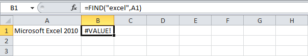
Функция FIND (НАЙТИ) и функция SEARCH (ПОИСК) очень похожи друг на друга. Этот пример демонстрирует разницу.
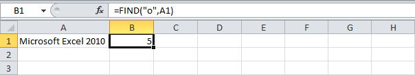
- Попробуйте использовать функцию FIND (НАЙТИ), чтобы найти положение подстроки в строке. Как видно на рисунке, эта функция чувствительна к регистру.
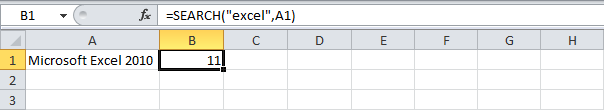
- Теперь испытайте функцию SEARCH (ПОИСК), чтобы найти положение искомого текста в строке. Эта функция не чувствительна к регистру.
Примечание: Текст «excel» имеет позицию 11 в данной строке, даже, если он используется немного в другом регистре («Excel»).
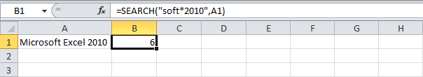
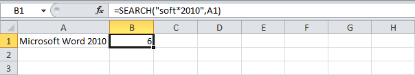
- Функция SEARCH (ПОИСК) более универсальна. Вы можете использовать подстановочные символы, когда применяете её.
Примечание: Вопросительный знак (?) соответствует ровно одному символу. Звездочка (*) соответствует ряду символов (от нуля и более).
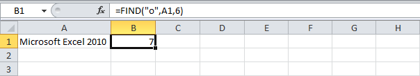
- Еще одна интересная особенность функций FIND (НАЙТИ) и SEARCH (ПОИСК) в том, что они имеют 3-й дополнительный аргумент. Вы можете использовать данный аргумент, чтобы задать позицию (начиная слева), с которой нужно начать поиск.
Примечание: Строка «o» найдена в позиции 5.
Примечание: Строка «o» найдена в позиции 7 (поиск начался с позиции 6).
Оцените качество статьи. Нам важно ваше мнение:
The FIND function and SEARCH function are somewhat similar, but still there is a factor that distinguishes them to be selective for solving our query in Microsoft Excel.
FIND function in Microsoft Excel returns the position of a specified character or sub-string within a string or text.
Syntax:- =FIND(find_text,within_text,[start_num])
SEARCH function returns the position of the first character of sub-string or search_text in a string. Syntax:- =SEARCH(find_text,within_text,[start_num])
In the below table, we can see the difference between both functions:-
| FIND | SEARCH |
|---|---|
| This function is case-sensitive | This function is not case-sensitive |
| It does not allow wildcard characters | It allows the wildcard characters such as «?», «*» etc. |
| This function search exact text | This function does not check uppercase and lowercase letters |
FIND Function
Let’s take examples and understand:-
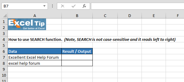
Let’s go to the Excel sheet. We have data sets in cell A7 & A8. And, we will put the function in cell B7 & B8 to get the desired output.

In the above example, we want to find the place number of the character “Excellent”, follow below given steps:-
- Enter the function in cell B7
- =FIND(«Excellent»,A7,1)
- Press Enter
- The function will return 1
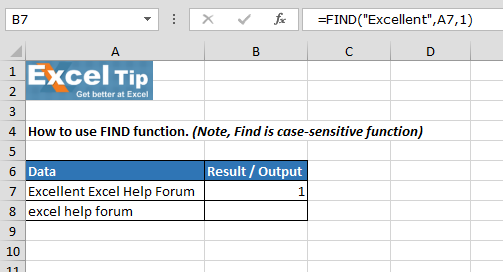
Formula Explanation: — First of all, find function will check the “Excellent” in the defined cell from the first position; from whatever position text will start, function will return as result. In the cell text, we can see that Excellent is starting from the first place of the cell text.
Let’s understand the case, in which function will not work
- Now enter the function in cell B8 to find out the “Excel”
- =FIND(«Excel»,A8,1)
- Press Enter, the function will return #VALUE! Error
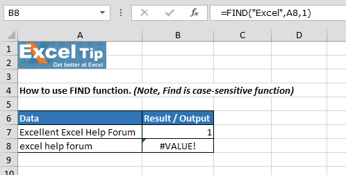
The function has given #VALUE! Error, because this function works is case-sensitive and, here in the function, we have mentioned “Excel”, and the same text is available in lower case in the cell.
SEARCH Function
First we want to find out the Excellent within a cell:-
- Enter the function in cell B7
- =SEARCH(«excellent»,A7,1)
- Press Enter
- The function will return 1

Note:- We haven’t defined the exact text for which we want to search the position.
Let’s understand the use of Wildcard characters in SEARCH function. Now, we will search for “Forum”
- Enter the function in cell B8
- =SEARCH(«?oru?»,A8,1)
- Press Enter
- The function will return 12
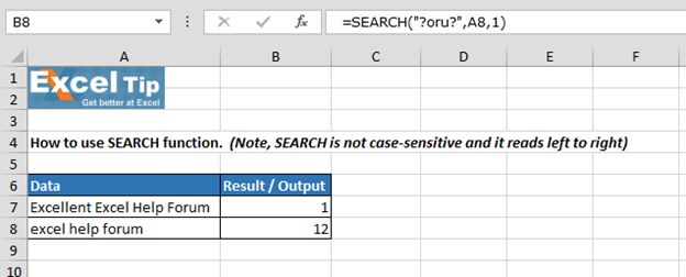
In this way, we can use wildcard character in SEARCH function to get the position number within cell text.
Note: — Another interesting point to mention about the FIND and the SEARCH function is that they have a 3rd optional argument. We can use this argument to indicate the position, counting from the left, from where we want to start searching.
![]()
If you liked our blogs, share it with your friends on Facebook. And also you can follow us on Twitter and Facebook.
We would love to hear from you, do let us know how we can improve, complement or innovate our work and make it better for you. Write us at info@exceltip.com
The two formulas FIND and SEARCH in Excel are very similar. They search through a cell or some text for a keyword or character. Once found, they return the number of characters, at which the keyword starts. Let’s learn how to use them and explore the differences of the two formulas.
How to use the FIND formula
The formula returns the number of the character, at which your search term starts. If your text can’t be found, it’ll return a “#VALUE” error.
Structure of the FIND formula
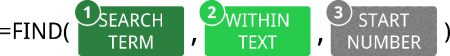
The structure of the FIND formula is quite simple (the numbers are corresponding to the image on the right-hand side):
- SEARCH TERM: The first part of the formula is the text you look for.
- WITHIN TEXT: The cell or text you want to search your “SEARCH TERM” in.
- START NUMBER: This argument is optional. If you don’t want to start searching at the beginning of the text, fill in the number larger than 1, otherwise just type 1 or leave it blank.
If you just want to know, if your text can be found within another cell, you might want to go with the following formula. B2 contains the text or character you search for and B3 is the cell you search in:
=IFERROR(IF(FIND(B2,B3)>0,”Value found”,””),”Value not found”)
Please note the following comments:
- FIND is case-sensitive. That means, it matters if you use small or capital letters.
- You can also search for numbers within another number. For example: =FIND(1,321)This formula returns 3 because the number 1 is the third character of 321.
- You can’t use wildcard criteria (“*” or “?”) with the FIND formula.
- Please refer to this article if you want to know more about the IF formula and to this article for more information about the IFERROR formula.
Examples for the FIND formula
Let’s try some examples.
Example 1: Find the first occurrence
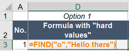
The “default” usage of the FIND formula is to return the number of characters, at which a text first occurs within another text. Let’s say you have the text “Hello there” and want to know, at which position you have an “o”. In such case, you write the following formula (example number 1 in the Excel workbook you can download at the end of this article).
=FIND(“o”,”Hello there”)
The return value is 5.
Example 2: Find the first occurrence after the third character
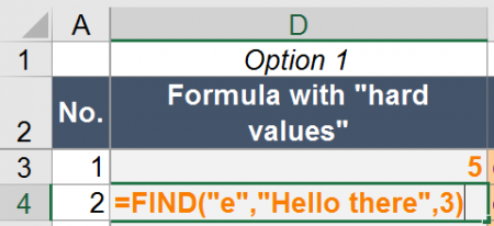
Another example: You want to know the position of “e” after the third character (example number 2 in the example workbook).
=FIND(“e”,”Hello there”,3)
The return value is 9.
Example 3: Find the second occurrence
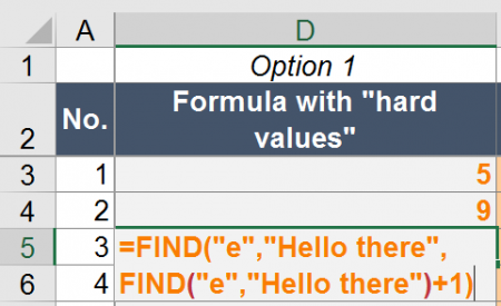
Now you want to know the position of the second occurrence of “e” in “Hello there”.
=FIND(“e”;”Hello there”;FIND(“e”;”Hello there”)+1)
This formula works as follows. The second FIND formula returns the position of the first occurrence of “e” in “Hello there” which is 2. This is used as the START NUMBER (+ 1 because you want to start counting after the first “e”) for the first FIND formula.
Example 4: Find the last occurrence
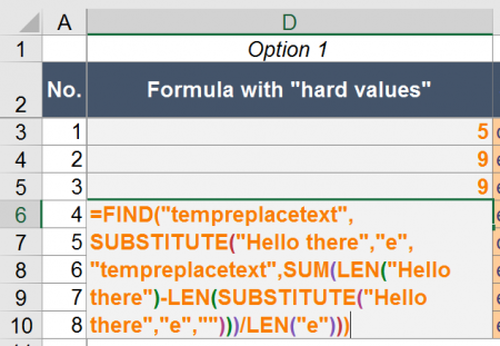
Finding the last occurrence of a string within a text is a little bit more complicated. You use SUBSTITUTE and LEN. The complete formula is like this:
=FIND(“tempreplacetext”;SUBSTITUTE(“Hello there”;”e”;”tempreplacetext”;SUM(LEN(“Hello there”)-LEN(SUBSTITUTE(“Hello there”;”e”;””)))/LEN(“e”)))
In order to understand the formula better, let’s start in the middle with the part SUM(LEN(“Hello there”)-LEN(SUBSTITUTE(“Hello there”;”e”;””)))/LEN(“e”)))
This part of the formula determines the number of “e” in “Hello there”. It replaces “e” in “Hello there” and the difference in the two versions (with and without e – “Hello there” and “Hllo thr”) is the number of “e”s.
The whole part SUBSTITUTE(“Hello there”;”e”;”tempreplacetext”;SUM(LEN(“Hello there”)-LEN(SUBSTITUTE(“Hello there”;”e”;””)))/LEN(“e”))) replaces the last “e” by “tempreplacetext”. Now you just put this into the FIND formula and get the position of “tempreplacetext”.
If you want to use this formula, replace all “e”s by your cell reference for the SEARCH TEXT and all “Hello there” by the cell reference to your WITHIN TEXT.
Replace text enclosed by brackets
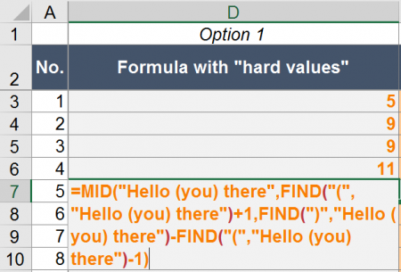
A last example for the FIND formula: You want to know what is written between two brackets. In such case, you can also use the FIND formulas in combination with the MID formula.
=MID(“Hello (you) there”,FIND(“(“,”Hello (you) there”)+1,FIND(“)”,”Hello (you) there”)-FIND(“(“,”Hello (you) there”)-1)
The MID formula returns some part of text from a (longer) text. It has three arguments:
- The initial, complete text.
- The starting character for the text you want to get.
- The length (in number of characters) of text you want to extract.
In our example above, the first FIND formula provides the character you want to start at. In our case that’s the first opening bracket (+1 because you want to start one character later). The second and third FIND formulas determine the length by
How to use the SEARCH formula
Like the FIND formula in Excel, SEARCH also returns the position of a text within another text.
Structure of the SEARCH formula

The SEARCH formula is very similar to the FIND formula. It has exactly the same arguments and works the same way.
Because of the, the structure is as follows:
- The SEARCH TERM is the text or character you search for.
- WITHIN TEXT contains the text you search in.
- The START NUMBER is optional and defines the number of character, after which Excel should start searching.
Yes, you are right – these arguments are exactly the same like in the FIND formula. But there is a major difference: SEARCH does not regard lower and upper case: It is not case sensitive. FIND on the other hand is case-sensitive and regards upper and lower cases.
Do you want to boost your productivity in Excel?
Get the Professor Excel ribbon!

Add more than 120 great features to Excel!
Examples for the SEARCH formula
The examples work exactly the same way like for the FIND formula. You only have to replace “FIND” by “SEARCH”. Because of that, we just show the summary below. If you want to know more, either scroll up to the “FIND”-examples or download the example workbook below.
| Example no. | Description | Formula |
| 6 | Return the position of “o” in “Hello there”. | =SEARCH(“o”,”Hello there”) |
| 7 | Return the position of “e” in “Hello there” after the third character. | =SEARCH(“e”,”Hello there”,3) |
| 8 | Return the position of the second occurrence of “e” in “Hello there”. | =SEARCH(“e”,”Hello there”,SEARCH(“e”,”Hello there”)+1) |
| 9 | Return the position of the last occurrence of “e” in “Hello there”. | =SEARCH(“tempreplacetext”,SUBSTITUTE(“Hello there”,”e”,”tempreplacetext”,SUM(LEN(“Hello there”)-LEN(SUBSTITUTE(“Hello there”,”e”,””)))/LEN(“e”))) |
| 10 | Return the text within brackets of “Hello (you) there”. | =MID(“Hello (you) there”,SEARCH(“(“,”Hello (you) there”)+1,SEARCH(“)”,”Hello (you) there”)-SEARCH(“(“,”Hello (you) there”)-1) |
Troubleshooting
The error message “#VALUE!” comes up most often for the FIND and SEARCH formulas. If you receive a “#VALUE!” error, please check the following possibilities.
- Make sure your SEARCH TERM can be found. If it can’t be found, you’ll receive the #VALUE! error.
- The last argument, the START NUMBER, is larger than the number of characters of in your WITHIN TEXT argument.
- You haven’t provided the last argument although you wrote the comma. For instance =SEARCH(“b”,”abc”,).
- Please check, if your SEARCH TERM and WITHIN TEXT have the same format. You can’t search for a letter or text in a number cell.
Difference between FIND and SEARCH
The first and major difference between FIND and SEARCH:
FIND is case-sensitive. SEARCH is not case-sensitive.
That means, FIND regards capital and small letter whereas SEARCH doesn’t.
How to remember which is which? I use the mnemonic:
- FIND finds exactly what you look for.
- Searching for something also searches for roughly what you look for.
I admit, it’s not the best mnemonic. Please let me know, if you have a better one!
There is also a second difference between FIND and SEARCH: You can use SEARCH with wildcard criteria within the SEARCH TERM.
- “?” stands for a single character. Example: =SEARCH(“?b”,”abc”)
- “*” matches any sequence of characters. =SEARCH(“*b”,”abc”)
- If you want to search exactly for ? or *, write a tilde in front of them. Example: =SEARCH(“~*”,”ab*c”)
Differences between FIND and FINDB as well as SEARCH and SEARCHB
Maybe you have noticed that there is also a slightly different version of the two formulas in Excel. If you add a “B” to the formulas, you can still use them the same way. So what is the difference?
FINDB and SEARCHB provide support for more complex languages. The definition by Microsoft is:
SEARCHB counts 2 bytes per character only when a DBCS language is set as the default language. Otherwise SEARCHB behaves the same as SEARCH, counting 1 byte per character.
According to Wikipedia DBCS stands mainly for the Asian languages Chinese, Japanese and Korean.
Please feel free to download all the examples shown above in this Excel file.
Click here and the download starts immediately.
Содержание
- SEARCH, SEARCHB functions
- Description
- Syntax
- Remark
- Examples
- FIND, FINDB functions
- Description
- Syntax
- Remarks
- Examples
- Функция НАЙТИ в Excel. Как использовать?
- Что возвращает функция
- Синтаксис
- Аргументы функции
- Дополнительная информация
- Примеры использования функции НАЙТИ в Excel
- Пример 1. Ищем слово в текстовой строке (с начала строки)
- Пример 2. Ищем слово в текстовой строке (с заданным порядковым номером старта поиска)
- Пример 3. Поиск текстового значения внутри текстовой строки с дублированным искомым значением
- FIND & SEARCH in Excel: How and When to Use These Formulas
- How to use the FIND formula
- Structure of the FIND formula
- Examples for the FIND formula
- Example 1: Find the first occurrence
- Example 2: Find the first occurrence after the third character
- Example 3: Find the second occurrence
- Example 4: Find the last occurrence
- Replace text enclosed by brackets
- How to use the SEARCH formula
- Structure of the SEARCH formula
- Examples for the SEARCH formula
- Troubleshooting
- Difference between FIND and SEARCH
- Differences between FIND and FINDB as well as SEARCH and SEARCHB
- Download
SEARCH, SEARCHB functions
This article describes the formula syntax and usage of the SEARCH and SEARCHB functions in Microsoft Excel.
Description
The SEARCH and SEARCHB functions locate one text string within a second text string, and return the number of the starting position of the first text string from the first character of the second text string. For example, to find the position of the letter «n» in the word «printer», you can use the following function:
This function returns 4 because «n» is the fourth character in the word «printer.»
You can also search for words within other words. For example, the function
returns 5, because the word «base» begins at the fifth character of the word «database». You can use the SEARCH and SEARCHB functions to determine the location of a character or text string within another text string, and then use the MID and MIDB functions to return the text, or use the REPLACE and REPLACEB functions to change the text. These functions are demonstrated in Example 1 in this article.
These functions may not be available in all languages.
SEARCHB counts 2 bytes per character only when a DBCS language is set as the default language. Otherwise SEARCHB behaves the same as SEARCH, counting 1 byte per character.
The languages that support DBCS include Japanese, Chinese (Simplified), Chinese (Traditional), and Korean.
Syntax
The SEARCH and SEARCHB functions have the following arguments:
find_text Required. The text that you want to find.
within_text Required. The text in which you want to search for the value of the find_text argument.
start_num Optional. The character number in the within_text argument at which you want to start searching.
The SEARCH and SEARCHB functions are not case sensitive. If you want to do a case sensitive search, you can use FIND and FINDB.
You can use the wildcard characters — the question mark ( ?) and asterisk ( *) — in the find_text argument. A question mark matches any single character; an asterisk matches any sequence of characters. If you want to find an actual question mark or asterisk, type a tilde (
) before the character.
If the value of find_text is not found, the #VALUE! error value is returned.
If the start_num argument is omitted, it is assumed to be 1.
If start_num is not greater than 0 (zero) or is greater than the length of the within_text argument, the #VALUE! error value is returned.
Use start_num to skip a specified number of characters. Using the SEARCH function as an example, suppose you are working with the text string «AYF0093.YoungMensApparel». To find the position of the first «Y» in the descriptive part of the text string, set start_num equal to 8 so that the serial number portion of the text (in this case, «AYF0093») is not searched. The SEARCH function starts the search operation at the eighth character position, finds the character that is specified in the find_text argument at the next position, and returns the number 9. The SEARCH function always returns the number of characters from the start of the within_text argument, counting the characters you skip if the start_num argument is greater than 1.
Examples
Copy the example data in the following table, and paste it in cell A1 of a new Excel worksheet. For formulas to show results, select them, press F2, and then press Enter. If you need to, you can adjust the column widths to see all the data.
Источник
FIND, FINDB functions
This article describes the formula syntax and usage of the FIND and FINDB functions in Microsoft Excel.
Description
FIND and FINDB locate one text string within a second text string, and return the number of the starting position of the first text string from the first character of the second text string.
These functions may not be available in all languages.
FIND is intended for use with languages that use the single-byte character set (SBCS), whereas FINDB is intended for use with languages that use the double-byte character set (DBCS). The default language setting on your computer affects the return value in the following way:
FIND always counts each character, whether single-byte or double-byte, as 1, no matter what the default language setting is.
FINDB counts each double-byte character as 2 when you have enabled the editing of a language that supports DBCS and then set it as the default language. Otherwise, FINDB counts each character as 1.
The languages that support DBCS include Japanese, Chinese (Simplified), Chinese (Traditional), and Korean.
Syntax
FIND(find_text, within_text, [start_num])
FINDB(find_text, within_text, [start_num])
The FIND and FINDB function syntax has the following arguments:
Find_text Required. The text you want to find.
Within_text Required. The text containing the text you want to find.
Start_num Optional. Specifies the character at which to start the search. The first character in within_text is character number 1. If you omit start_num, it is assumed to be 1.
FIND and FINDB are case sensitive and don’t allow wildcard characters. If you don’t want to do a case sensitive search or use wildcard characters, you can use SEARCH and SEARCHB.
If find_text is «» (empty text), FIND matches the first character in the search string (that is, the character numbered start_num or 1).
Find_text cannot contain any wildcard characters.
If find_text does not appear in within_text, FIND and FINDB return the #VALUE! error value.
If start_num is not greater than zero, FIND and FINDB return the #VALUE! error value.
If start_num is greater than the length of within_text, FIND and FINDB return the #VALUE! error value.
Use start_num to skip a specified number of characters. Using FIND as an example, suppose you are working with the text string «AYF0093.YoungMensApparel». To find the number of the first «Y» in the descriptive part of the text string, set start_num equal to 8 so that the serial-number portion of the text is not searched. FIND begins with character 8, finds find_text at the next character, and returns the number 9. FIND always returns the number of characters from the start of within_text, counting the characters you skip if start_num is greater than 1.
Examples
Copy the example data in the following table, and paste it in cell A1 of a new Excel worksheet. For formulas to show results, select them, press F2, and then press Enter. If you need to, you can adjust the column widths to see all the data.
Источник
Функция НАЙТИ в Excel. Как использовать?
Функция НАЙТИ (FIND) в Excel используется для поиска текстового значения внутри строчки с текстом и указать порядковый номер буквы с которого начинается искомое слово в найденной строке.
Что возвращает функция
Возвращает числовое значение, обозначающее стартовую позицию текстовой строчки внутри другой текстовой строчки.
Синтаксис
=FIND(find_text, within_text, [start_num]) — английская версия
=НАЙТИ(искомый_текст;просматриваемый_текст;[нач_позиция]) — русская версия
Аргументы функции
- find_text (искомый_текст) — текст или строка которую вы хотите найти в рамках другой строки;
- within_text (просматриваемый_текст) — текст, внутри которого вы хотите найти аргумент find_text (искомый_текст);
- [start_num] ([нач_позиция]) — число, отображающее позицию, с которой вы хотите начать поиск. Если аргумент не указать, то поиск начнется сначала.
Дополнительная информация
- Если стартовое число не указано, то функция начинает поиск искомого текста с начала строки;
- Функция НАЙТИ чувствительна к регистру. Если вы хотите сделать поиск без учета регистра, используйте функцию SEARCH в Excel;
- Функция не учитывает подстановочные знаки при поиске. Если вы хотите использовать подстановочные знаки для поиска, используйте функцию SEARCH в Excel;
- Функция каждый раз возвращает ошибку, когда не находит искомый текст в заданной строке.
Примеры использования функции НАЙТИ в Excel
Пример 1. Ищем слово в текстовой строке (с начала строки)
![]()
На примере выше мы ищем слово «Доброе» в словосочетании «Доброе Утро». По результатам поиска, функция выдает число «1», которое обозначает, что слово «Доброе» начинается с первой по очереди буквы в, заданной в качестве области поиска, текстовой строке.
Обратите внимание, что так как функция НАЙТИ в Excel чувствительна к регистру, вы не сможете найти слово «доброе» в словосочетании «Доброе утро», так как оно написано с маленькой буквы. Для того, чтобы осуществить поиска без учета регистра следует пользоваться функцией SEARCH .
Пример 2. Ищем слово в текстовой строке (с заданным порядковым номером старта поиска)
![]()
Третий аргумент функции НАЙТИ указывает позицию, с которой функция начинает поиск искомого значения. На примере выше функция возвращает число «1» когда мы начинаем поиск слова «Доброе» в словосочетании «Доброе утро» с начала текстовой строки. Но если мы зададим аргумент функции start_num (нач_позиция) со значением «2», то функция выдаст ошибку, так как начиная поиск со второй буквы текстовой строки, она не может ничего найти.
Если вы не укажете номер позиции, с которой функции следует начинать поиск искомого аргумента, то Excel по умолчанию начнет поиск с самого начала текстовой строки.
Пример 3. Поиск текстового значения внутри текстовой строки с дублированным искомым значением
![]()
На примере выше мы ищем слово «Доброе» в словосочетании «Доброе Доброе утро». Когда мы начинаем поиск слова «Доброе» с начала текстовой строки, то функция выдает число «1», так как первое слово «Доброе» начинается с первой буквы в словосочетании «Доброе Доброе утро».
Но, если мы укажем в качестве аргумента start_num (нач_позиция) число «2» и попросим функцию начать поиск со второй буквы в заданной текстовой строке, то функция выдаст число «6», так как Excel находит искомое слово «Доброе» начиная со второй буквы словосочетания «Доброе Доброе утро» только на 6 позиции.
Источник
FIND & SEARCH in Excel: How and When to Use These Formulas
The two formulas FIND and SEARCH in Excel are very similar. They search through a cell or some text for a keyword or character. Once found, they return the number of characters, at which the keyword starts. Let’s learn how to use them and explore the differences of the two formulas.
How to use the FIND formula
The formula returns the number of the character, at which your search term starts. If your text can’t be found, it’ll return a “#VALUE” error.
Structure of the FIND formula
The structure of the FIND formula is quite simple (the numbers are corresponding to the image on the right-hand side):
- SEARCH TERM: The first part of the formula is the text you look for.
- WITHIN TEXT: The cell or text you want to search your “SEARCH TERM” in.
- START NUMBER: This argument is optional. If you don’t want to start searching at the beginning of the text, fill in the number larger than 1, otherwise just type 1 or leave it blank.
If you just want to know, if your text can be found within another cell, you might want to go with the following formula. B2 contains the text or character you search for and B3 is the cell you search in:
=IFERROR(IF(FIND(B2,B3)>0,”Value found”,””),”Value not found”)
Please note the following comments:
- FIND is case-sensitive. That means, it matters if you use small or capital letters.
- You can also search for numbers within another number. For example: =FIND(1,321) This formula returns 3 because the number 1 is the third character of 321.
- You can’t use wildcard criteria (“*” or “?”) with the FIND formula.
- Please refer to this article if you want to know more about the IF formula and to this article for more information about the IFERROR formula.
Examples for the FIND formula
Let’s try some examples.
Example 1: Find the first occurrence
The “default” usage of the FIND formula is to return the number of characters, at which a text first occurs within another text. Let’s say you have the text “Hello there” and want to know, at which position you have an “o”. In such case, you write the following formula (example number 1 in the Excel workbook you can download at the end of this article).
The return value is 5.
Example 2: Find the first occurrence after the third character
Another example: You want to know the position of “e” after the third character (example number 2 in the example workbook).
The return value is 9.
Example 3: Find the second occurrence
Now you want to know the position of the second occurrence of “e” in “Hello there”.
=FIND(“e”;”Hello there”;FIND(“e”;”Hello there”)+1)
This formula works as follows. The second FIND formula returns the position of the first occurrence of “e” in “Hello there” which is 2. This is used as the START NUMBER (+ 1 because you want to start counting after the first “e”) for the first FIND formula.
Example 4: Find the last occurrence
Finding the last occurrence of a string within a text is a little bit more complicated. You use SUBSTITUTE and LEN. The complete formula is like this:
=FIND(“tempreplacetext”;SUBSTITUTE(“Hello there”;”e”;”tempreplacetext”;SUM(LEN(“Hello there”)-LEN(SUBSTITUTE(“Hello there”;”e”;””)))/LEN(“e”)))
In order to understand the formula better, let’s start in the middle with the part SUM(LEN(“Hello there”)-LEN(SUBSTITUTE(“Hello there”;”e”;””)))/LEN(“e”)))
This part of the formula determines the number of “e” in “Hello there”. It replaces “e” in “Hello there” and the difference in the two versions (with and without e – “Hello there” and “Hllo thr”) is the number of “e”s.
The whole part SUBSTITUTE(“Hello there”;”e”;”tempreplacetext”;SUM(LEN(“Hello there”)-LEN(SUBSTITUTE(“Hello there”;”e”;””)))/LEN(“e”))) replaces the last “e” by “tempreplacetext”. Now you just put this into the FIND formula and get the position of “tempreplacetext”.
If you want to use this formula, replace all “e”s by your cell reference for the SEARCH TEXT and all “Hello there” by the cell reference to your WITHIN TEXT.
Replace text enclosed by brackets
A last example for the FIND formula: You want to know what is written between two brackets. In such case, you can also use the FIND formulas in combination with the MID formula.
=MID(“Hello (you) there”,FIND(“(“,”Hello (you) there”)+1,FIND(“)”,”Hello (you) there”)-FIND(“(“,”Hello (you) there”)-1)
The MID formula returns some part of text from a (longer) text. It has three arguments:
- The initial, complete text.
- The starting character for the text you want to get.
- The length (in number of characters) of text you want to extract.
In our example above, the first FIND formula provides the character you want to start at. In our case that’s the first opening bracket (+1 because you want to start one character later). The second and third FIND formulas determine the length by
How to use the SEARCH formula
Like the FIND formula in Excel, SEARCH also returns the position of a text within another text.
Structure of the SEARCH formula
The SEARCH formula is very similar to the FIND formula. It has exactly the same arguments and works the same way.
Because of the, the structure is as follows:
- The SEARCH TERM is the text or character you search for.
- WITHIN TEXT contains the text you search in.
- The START NUMBER is optional and defines the number of character, after which Excel should start searching.
Yes, you are right – these arguments are exactly the same like in the FIND formula. But there is a major difference: SEARCH does not regard lower and upper case: It is not case sensitive. FIND on the other hand is case-sensitive and regards upper and lower cases.
Do you want to boost your productivity in Excel?
Get the Professor Excel ribbon!
Add more than 120 great features to Excel!
Examples for the SEARCH formula
The examples work exactly the same way like for the FIND formula. You only have to replace “FIND” by “SEARCH”. Because of that, we just show the summary below. If you want to know more, either scroll up to the “FIND”-examples or download the example workbook below.
| Example no. | Description | Formula |
| 6 | Return the position of “o” in “Hello there”. | =SEARCH(“o”,”Hello there”) |
| 7 | Return the position of “e” in “Hello there” after the third character. | =SEARCH(“e”,”Hello there”,3) |
| 8 | Return the position of the second occurrence of “e” in “Hello there”. | =SEARCH(“e”,”Hello there”,SEARCH(“e”,”Hello there”)+1) |
| 9 | Return the position of the last occurrence of “e” in “Hello there”. | =SEARCH(“tempreplacetext”,SUBSTITUTE(“Hello there”,”e”,”tempreplacetext”,SUM(LEN(“Hello there”)-LEN(SUBSTITUTE(“Hello there”,”e”,””)))/LEN(“e”))) |
| 10 | Return the text within brackets of “Hello (you) there”. | =MID(“Hello (you) there”,SEARCH(“(“,”Hello (you) there”)+1,SEARCH(“)”,”Hello (you) there”)-SEARCH(“(“,”Hello (you) there”)-1) |
Troubleshooting
The error message “#VALUE!” comes up most often for the FIND and SEARCH formulas. If you receive a “#VALUE!” error, please check the following possibilities.
- Make sure your SEARCH TERM can be found. If it can’t be found, you’ll receive the #VALUE! error.
- The last argument, the START NUMBER, is larger than the number of characters of in your WITHIN TEXT argument.
- You haven’t provided the last argument although you wrote the comma. For instance =SEARCH(“b”,”abc”,).
- Please check, if your SEARCH TERM and WITHIN TEXT have the same format. You can’t search for a letter or text in a number cell.
Difference between FIND and SEARCH
The first and major difference between FIND and SEARCH:
FIND is case-sensitive. SEARCH is not case-sensitive.
That means, FIND regards capital and small letter whereas SEARCH doesn’t.
How to remember which is which? I use the mnemonic:
- FIND finds exactly what you look for.
- Searching for something also searches for roughly what you look for.
I admit, it’s not the best mnemonic. Please let me know, if you have a better one!
There is also a second difference between FIND and SEARCH: You can use SEARCH with wildcard criteria within the SEARCH TERM.
- “?” stands for a single character. Example: =SEARCH(“?b”,”abc”)
- “*” matches any sequence of characters. =SEARCH(“*b”,”abc”)
- If you want to search exactly for ? or *, write a tilde in front of them. Example: =SEARCH(“
Differences between FIND and FINDB as well as SEARCH and SEARCHB
Maybe you have noticed that there is also a slightly different version of the two formulas in Excel. If you add a “B” to the formulas, you can still use them the same way. So what is the difference?
FINDB and SEARCHB provide support for more complex languages. The definition by Microsoft is:
SEARCHB counts 2 bytes per character only when a DBCS language is set as the default language. Otherwise SEARCHB behaves the same as SEARCH, counting 1 byte per character.
According to Wikipedia DBCS stands mainly for the Asian languages Chinese, Japanese and Korean.
Download
Please feel free to download all the examples shown above in this Excel file.
Click here and the download starts immediately.
Источник