Find and replace formula for excel

Use the Find and Replace features in Excel to search for something in your workbook, such as a particular number or text string. You can either locate the search item for reference, or you can replace it with something else. You can include wildcard characters such as question marks, tildes, and asterisks, or numbers in your search terms. You can search by rows and columns, search within comments or values, and search within worksheets or entire workbooks.

Find

To find something, press Ctrl+F, or go to Home > Editing > Find & Select > Find.

Note: In the following example, we’ve clicked the Options >> button to show the entire Find dialog. By default, it will display with Options hidden.

In the Find what: box, type the text or numbers you want to find, or click the arrow in the Find what: box, and then select a recent search item from the list.
Tips: You can use wildcard characters — question mark (?), asterisk (*), tilde (~) — in your search criteria.
- Use the question mark (?) to find any single character — for example, s?t finds «sat» and «set».
- Use the asterisk (*) to find any number of characters — for example, s*d finds «sad» and «started».
- Use the tilde (~) followed by ?, *, or ~ to find question marks, asterisks, or other tilde characters — for example, fy91~? finds «fy91?».
Click Find All or Find Next to run your search.

Tip: When you click Find All, every occurrence of the criteria that you are searching for will be listed, and clicking a specific occurrence in the list will select its cell. You can sort the results of a Find All search by clicking a column heading.
Click Options>> to further define your search if needed:
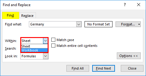
- Within: To search for data in a worksheet or in an entire workbook, select Sheet or Workbook.
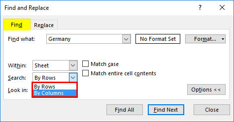
- Search: You can choose to search either By Rows (default), or By Columns.
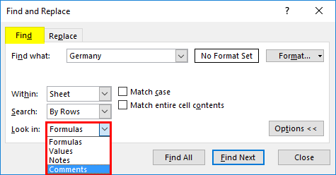
- Look in: To search for data with specific details, in the box, click Formulas, Values, Notes, or Comments.
  
  Note: Formulas, Values, Notes and Comments are only available on the Find tab; only Formulas are available on the Replace tab.
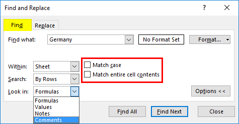
- Match case — Check this if you want to search for case-sensitive data.
- Match entire cell contents — Check this if you want to search for cells that contain just the characters that you typed in the Find what: box.
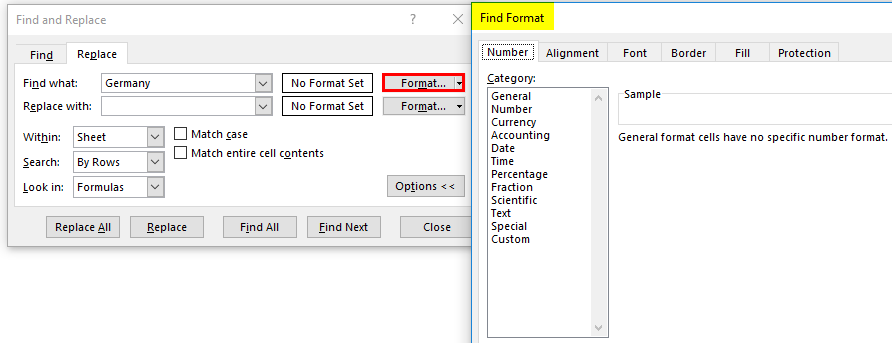
If you want to search for text or numbers with specific formatting, click Format, and then make your selections in the Find Format dialog box.

Tip: If you want to find cells that just match a specific format, you can delete any criteria in the Find what box, and then select a specific cell format as an example. Click the arrow next to Format, click Choose Format From Cell, and then click the cell that has the formatting that you want to search for.

Replace

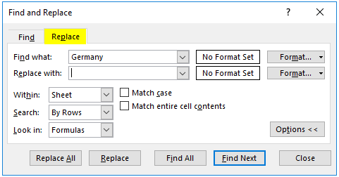
To replace text or numbers, press Ctrl+H, or go to Home > Editing > Find & Select > Replace.

Note: In the following example, we’ve clicked the Options >> button to show the entire Find dialog. By default, it will display with Options hidden.

In the Find what: box, type the text or numbers you want to find, or click the arrow in the Find what: box, and then select a recent search item from the list.
Tips: You can use wildcard characters — question mark (?), asterisk (*), tilde (~) — in your search criteria.
- Use the question mark (?) to find any single character — for example, s?t finds «sat» and «set».
- Use the asterisk (*) to find any number of characters — for example, s*d finds «sad» and «started».
- Use the tilde (~) followed by ?, *, or ~ to find question marks, asterisks, or other tilde characters — for example, fy91~? finds «fy91?».
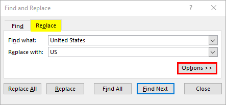
In the Replace with: box, enter the text or numbers you want to use to replace the search text.
Click Replace All or Replace.

Tip: When you click Replace All, every occurrence of the criteria that you are searching for will be replaced, while Replace will update one occurrence at a time.
Click Options>> to further define your search if needed:
- Within: To search for data in a worksheet or in an entire workbook, select Sheet or Workbook.
- Search: You can choose to search either By Rows (default), or By Columns.
- Look in: To search for data with specific details, in the box, click Formulas, Values, Notes, or Comments.
  
  Note: Formulas, Values, Notes and Comments are only available on the Find tab; only Formulas are available on the Replace tab.
- Match case — Check this if you want to search for case-sensitive data.
- Match entire cell contents — Check this if you want to search for cells that contain just the characters that you typed in the Find what: box.
If you want to search for text or numbers with specific formatting, click Format, and then make your selections in the Find Format dialog box.

Tip: If you want to find cells that just match a specific format, you can delete any criteria in the Find what box, and then select a specific cell format as an example. Click the arrow next to Format, click Choose Format From Cell, and then click the cell that has the formatting that you want to search for.

There are two distinct methods for finding or replacing text or numbers on the Mac. The first is to use the Find & Replace dialog. The second is to use the Search bar in the ribbon.

Find & Replace dialog

Search bar and options

Press Ctrl+F or go to Home > Find & Select > Find.
In Find what: type the text or numbers you want to find.
Select Find Next to run your search.
You can further define your search:
- Within: To search for data in a worksheet or in an entire workbook, select Sheet or Workbook.
- Search: You can choose to search either By Rows (default), or By Columns.
- Look in: To search for data with specific details, in the box, click Formulas, Values, Notes, or Comments.
- Match case — Check this if you want to search for case-sensitive data.
- Match entire cell contents — Check this if you want to search for cells that contain just the characters that you typed in the Find what: box.

Tips: You can use wildcard characters — question mark (?), asterisk (*), tilde (~) — in your search criteria.

Use the question mark (?) to find any single character — for example, s?t finds «sat» and «set».
Use the asterisk (*) to find any number of characters — for example, s*d finds «sad» and «started».
Use the tilde (~) followed by ?, *, or ~ to find question marks, asterisks, or other tilde characters — for example, fy91~? finds «fy91?».

Press Ctrl+F or go to Home > Find & Select > Find.
In Find what: type the text or numbers you want to find.
Select Find All to run your search for all occurrences.

Note: The dialog box expands to show a list of all the cells that contain the search term, and the total number of cells in which it appears.
Select any item in the list to highlight the corresponding cell in your worksheet.

Note: You can edit the contents of the highlighted cell.

Press Ctrl+H or go to Home > Find & Select > Replace.
In Find what, type the text or numbers you want to find.
You can further define your search:
- Within: To search for data in a worksheet or in an entire workbook, select Sheet or Workbook.
- Search: You can choose to search either By Rows (default), or By Columns.
- Match case — Check this if you want to search for case-sensitive data.
- Match entire cell contents — Check this if you want to search for cells that contain just the characters that you typed in the Find what: box.
  Tips: You can use wildcard characters — question mark (?), asterisk (*), tilde (~) — in your search criteria.
  - Use the question mark (?) to find any single character — for example, s?t finds «sat» and «set».
  - Use the asterisk (*) to find any number of characters — for example, s*d finds «sad» and «started».
  - Use the tilde (~) followed by ?, *, or ~ to find question marks, asterisks, or other tilde characters — for example, fy91~? finds «fy91?».
In the Replace with box, enter the text or numbers you want to use to replace the search text.
Select Replace or Replace All.
Tips:
- When you select Replace All, every occurrence of the criteria that you are searching for is replaced.
- When you select Replace, you can replace one instance at a time by selecting Next to highlight the next instance.

Select any cell to search the entire sheet or select a specific range of cells to search.
Press Command + F or select the magnifying glass to expand the Search bar and type the text or number you want to find in the search field.
Tips: You can use wildcard characters — question mark (?), asterisk (*), tilde (~) — in your search criteria.
- Use the question mark (?) to find any single character — for example, s?t finds «sat» and «set».
- Use the asterisk (*) to find any number of characters — for example, s*d finds «sad» and «started».
- Use the tilde (~) followed by ?, *, or ~ to find question marks, asterisks, or other tilde characters — for example, fy91~? finds «fy91?».
Press return.
Notes:
- To find the next instance of the item you are searching for, press return again or use the Find dialog box and select Find Next.
- To specify additional search options, select the magnifying glass and select Search in Sheet or Search in Workbook. You can also select the Advanced option, which launches the Find dialog.
Tip: You can cancel a search in progress by pressing ESC.

Find

To find something, press Ctrl+F, or go to Home > Editing > Find & Select > Find.

Note: In the following example, we’ve clicked > Search Options to show the entire Find dialog. By default, it will display with Search Options hidden.

In the Find what: box, type the text or numbers you want to find.
Tips: You can use wildcard characters — question mark (?), asterisk (*), tilde (~) — in your search criteria.
- Use the question mark (?) to find any single character — for example, s?t finds «sat» and «set».
- Use the asterisk (*) to find any number of characters — for example, s*d finds «sad» and «started».
- Use the tilde (~) followed by ?, *, or ~ to find question marks, asterisks, or other tilde characters — for example, fy91~? finds «fy91?».
Click Find Next or Find All to run your search.

Tip: When you click Find All, every occurrence of the criteria that you are searching for will be listed, and clicking a specific occurrence in the list will select its cell. You can sort the results of a Find All search by clicking a column heading.
Click > Search Options to further define your search if needed:
- Within: To search for data within a certain selection, choose Selection. To search for data in a worksheet or in an entire workbook, select Sheet or Workbook.
- Direction: You can choose to search either Down (default), or Up.
- Match case — Check this if you want to search for case-sensitive data.
- Match entire cell contents — Check this if you want to search for cells that contain just the characters that you typed in the Find what box.

Replace

To replace text or numbers, press Ctrl+H, or go to Home > Editing > Find & Select > Replace.

Note: In the following example, we’ve clicked > Search Options to show the entire Find dialog. By default, it will display with Search Options hidden.

In the Find what: box, type the text or numbers you want to find.
Tips: You can use wildcard characters — question mark (?), asterisk (*), tilde (~) — in your search criteria.
- Use the question mark (?) to find any single character — for example, s?t finds «sat» and «set».
- Use the asterisk (*) to find any number of characters — for example, s*d finds «sad» and «started».
- Use the tilde (~) followed by ?, *, or ~ to find question marks, asterisks, or other tilde characters — for example, fy91~? finds «fy91?».
In the Replace with: box, enter the text or numbers you want to use to replace the search text.
Click Replace or Replace All.

Tip: When you click Replace All, every occurrence of the criteria that you are searching for will be replaced, while Replace will update one occurrence at a time.
Click > Search Options to further define your search if needed:
- Within: To search for data within a certain selection, choose Selection. To search for data in a worksheet or in an entire workbook, select Sheet or Workbook.
- Direction: You can choose to search either Down (default), or Up.
- Match case — Check this if you want to search for case-sensitive data.
- Match entire cell contents — Check this if you want to search for cells that contain just the characters that you typed in the Find what box.

Need more help?

You can always ask an expert in the Excel Tech Community or get support in the Answers community.

What is Find and Replace Feature in Excel?

The Find and Replace feature of Excel looks for a data value and replaces it with another data value. This data value can be a text string, number, date or special character. The Find and Replace feature can search within a worksheet or workbook, by rows or columns, and within formulas, values or comments.

For example, in a financial report of Excel, the text string “asset” may need to be replaced with “assets.”

The purpose of using the Find and Replace feature in Excel is to locate certain information in a database. It also allows modifying the existing data values with a few clicks. By default, the Find and Replace excel feature looks for a partial match. But, it can also look for an exact match if the option “match entire cell contents” is selected.

What is Find and Replace Feature in Excel?
- How to Access the Find and Replace Feature of Excel?
  - Example #1–Find a Partial Match in a Worksheet
  - Example #2–Find a Partial Match in a Workbook
  - Example #3–Find an Exact Match in a Workbook
  - Example #4–Replace the Range Reference of a Formula
  - Example #5–Replace the Existing Text to Make Two Strings Identical
  - Example #6–Replace the Old Formatting of a Cell
  - Example #7–Find a Comment in a Worksheet
- The Key Points Related to the Find and Replace Feature of Excel
- Frequently Asked Questions
- Recommended Articles

How to Access the Find and Replace Feature of Excel?

The shortcuts to the Find and Replace excel feature are stated as follows:

“Ctrl+F” opens the Find tab of the Find and Replace feature.
“Ctrl+H” opens the Replace tab of the Find and Replace feature.

Alternatively, the “find” and “replace” options can be clicked from the “find & select” drop-down (“editing” group) of the Home tab. These options open the Find and Replace tabs of the Find and Replace feature of Excel.

Let us consider some examples to understand the working of the Find and Replace feature of Excel.

You can download this Find and Replace Excel Template here – Find and Replace Excel Template

Example #1–Find a Partial Match in a Worksheet

The following image shows two worksheets titled “Jan” and “Feb.” These worksheets contain datasets that report the sales made (column C) to different customers (column B) in January and February.

The names of the products, cost of goods sold (COGS), profits, and regions are also displayed in columns A, D, E, and F respectively. A similar dataset (with different numbers) is in columns H to M as well.

Find the name “Mitchel” in the worksheet “Jan.” Use the Find and Replace feature of Excel.

The steps to use find and replace function in excel is follows:

Go to the worksheet “Jan.” Next, press the keys “Ctrl+F” together. The Find tab of the “find and replace” dialog box opens. This is shown in the following image.
Note: By default, Excel searches in the currently active worksheet.
Type the word to be searched in the “find what” box. We type “Mitchel.”

Note that this search is not case-sensitive. So, even if the worksheet contains “MITCHEL,” it will show up in the search results.
Press either the “Enter” key or the “find next” option. The first occurrence of the name “Daniel Mitchel” is selected. So, cell B7 is selected, as shown in the following image. Clicking “find next” again and again selects the subsequent occurrences of “Mitchel.”
Notice that though we entered “Mitchel” in the “find what” box, Excel has selected the name “Daniel Mitchel.” This is called a partial match. It implies that if there are any additional words preceding or succeeding the search value, the entire string containing the search value is returned in the result.
Click “find all” to see all the strings containing “Mitchel.” The results are shown in the following image. These results display the following information:
• The column “book” displays the name of the workbook containing the search value.
• The column “sheet” displays the name of the worksheet containing the search value.
• The column “cell” displays the reference of the cells containing the search value.
• The column “value” displays the entire string containing the search value.

Notice that at the bottom of the dialog box, Excel displays the number of cells containing the search value. In this case, there are 8 cells in the worksheet “Jan,” which contain either “Mitchel” or “Daniel Mitchel.”

Difference between “find all” and “find next”: The “find all” option shows all the occurrences of the search value. Further, clicking any of the entries shown by this option takes the user to the corresponding cell.

The “find next” option helps scan through the different cells containing the search value. Clicking “find next” for the first time selects the first occurrence of the search value. Likewise, clicking “find next” the second time selects the second occurrence of the search value, and so on.

Example #2–Find a Partial Match in a Workbook

Working on the dataset of example #1, find the name “Mitchel” in the entire workbook. Use the Find and Replace feature of Excel.

The steps to search the stated string in the entire workbook are listed as follows:

Step 1: Press the keys “Ctrl+F” together. The Find tab of the “find and replace” window opens. Type the name “Mitchel” in the “find what” box.

Next, click “options,” shown within a black box in the following image.

Step 2: Clicking “options” expands the “find and replace” dialog box. Click the drop-down next to the option “within” and select “workbook.”

The selection is shown in the following image.

Step 3: Click “find all” to see all the results. The results are shown in the following image. This time the string “Mitchel” has been found in 16 cells of the workbook.

Clicking any of the entries will select the respective cell.

Example #3–Find an Exact Match in a Workbook

Working on the dataset of example #1, find an exact match of “Mitchel” in the entire workbook. Use the Find and Replace feature of Excel.

The steps to search the exact name in the entire workbook are listed as follows:

Step 1: Press the keys “Ctrl+F.” In the Find tab of the “find and replace” window, perform the following tasks:

Click “options” to expand the “find and replace” window.
Enter the name “Mitchel” in the “find what” box.
Select “workbook” in the box adjacent to “within.”
Select the checkbox of “match entire cell contents.”
Leave the “search” and “look in” parameters to default values which are “by rows” and “formulas” respectively.

The name of the “find what” box and the selections are shown in the following image.

Note: When the option “match entire cell contents” is selected, the Find and Replace excel feature looks for exactly those data values that have been entered in the “find what” box.

Step 2: Click “find all” to view all the exact matches of the name “Mitchel.” In the current workbook, 8 cells contain the exact name.

The results (shown in the following image) display the cell references, exact value, and the names of the worksheet and the workbook.

Example #4–Replace the Range Reference of a Formula

The following image shows the names (column A), salaries per annum (in $ in column B), salaries per month (in $ in column C), and departments (column D) of some employees of an organization.

The total salary per annum is shown in cell G3. This sum incorrectly considers the range B2:B10 in place of the range B2:B22. Rectify the range of the formulas in cells G3 and H3 so that the total salary per annum is calculated accurately. Use the Find and Replace feature of Excel.

The steps to edit a formula by using the Find and Replace feature of Excel are listed as follows:

Step 1: Copy the SUMThe SUM function in excel adds the numerical values in a range of cells. Being categorized under the Math and Trigonometry function, it is entered by typing “=SUM” followed by the values to be summed. The values supplied to the function can be numbers, cell references or ranges.read more formula of cell G3. For this, perform the given tasks:

Select cell G3. The formula [=SUM(B2:B10)] appears in the formula bar.
Copy this formula by pressing the keys “Ctrl+C” together.
Press the Escape (Esc) key once the formula has been copied. This will help exit the formula bar.

Alternatively, copy the formula of cell H3 by pressing the keys “Ctrl+C.” Next, press “Ctrl+H.”

Step 2: The Replace tab of the “find and replace” window opens. Paste the copied formula in the “find what” box, as shown in the following image. For pasting the formula, press the keys “Ctrl+V” together.

Note: Instead of copying and pasting, one can type the formula directly in the “find what” box.

Step 3: Enter the correct formula in the “replace with” box. So, type the formula “=SUM(B2:B22)” without the beginning and ending double quotation marks. This is shown in the following image.

Next, click “replace all.”

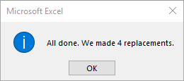
Step 4: Click “Ok” in the message stating the number of replacements made. The formulas of cells G3 and H3 change from “=SUM(B2:B10)” to “=SUM(B2:B22).” As a result, the total salary per annum changes.

The new output is shown within a red box in the following image. Hence, the total salary paid to the given 21 employees is $11,179,954 per annum.

Example #5–Replace the Existing Text to Make Two Strings Identical

There are two images titled “image 1” and “image 2.” Both images are in different worksheets. Further, the following information is given:

Image 1 shows the product code (column A) and prices (in $ in column B) of 21 products of a multinational organization.
Image 2 shows the product code (column A) and a blank column (column B) for the prices of the 21 products.

Notice that the product codes of both images consist of some letters prefixed to a number. The letters are different in both images, but the subsequent numbers are the same.

Make the product code identical in both images by using the Find and Replace feature of Excel. This will help fetch the prices of “image 1” in “image 2” (column B) with the VLOOKUP functionThe VLOOKUP excel function searches for a particular value and returns a corresponding match based on a unique identifier. A unique identifier is uniquely associated with all the records of the database. For instance, employee ID, student roll number, customer contact number, seller email address, etc., are unique identifiers.
read more.

Image 1

Image 2

The steps to make the product code identical by using the Find and Replace feature of Excel are listed as follows:

Step 1: Press the keys “Ctrl+H” to open the Replace tab of the “find and replace” window.

Step 2: Enter “pdc” in the “find what” box. Enter “prdct” in the “replace with” box. Next, click “replace all.” A message stating the number of replacements made is displayed. Click “Ok” to proceed.

The entries and the outputs are shown in the following image. Now, one can easily apply the VLOOKUP function to fetch the prices in this image. Had the replacements not been made, the VLOOKUP function could not have been applied.

Difference between “replace all” and “replace”: The “replace all” option replaces all the occurrences of the search value in one go. In contrast, the “replace” option replaces one occurrence at a time.

Therefore, use “replace” when not sure which occurrence needs to be replaced. Use “replace all” when all occurrences of the search value need to be replaced.

Example #6–Replace the Old Formatting of a Cell

The following image shows some departments of an organization. Cell A4 is in grey and cells B5, C2, and D5 are in blue. We want all the cells containing “marketing” to be in one color.

Therefore, replace the grey color of cell A4 with blue color. Use the Find and Replace feature of Excel.

The steps to change the formatting with the Find and Replace feature of Excel are listed as follows:

Step 1: Select the dataset whose formatting needs to be changed. We have selected the range A2:D6.

Next, press the keys “Ctrl+H” to open the Replace tab of the “find and replace” window. In this tab, click “options” shown on the right side.

This entire step is shown in the following image.

Step 2: Once “options” is clicked, the “find and replace” window expands. Click the drop-down arrow of the first “format” option (to the right of the “find what” box). Next, select “choose format from cell.”

The selection is shown within a black box in the following image.

Step 3: Select the cell whose formatting needs to be changed. We select cell A4. As a result, the “no format set” on the left of “format” changes to “preview.” This “preview” option reflects the color of cell A4, as shown in the following image.

Note: The “preview” option of the following image and cell A4 of the first image (at the beginning of this example) show a slight variation in color. Please ignore this variation, which may be due to different Excel versions being used to create images.

Step 4: Click the drop-down arrow of the second “format” option (to the right of the “replace with” box). Select “choose format from cell” and click any of the blue cells (B5, C2 or D5). Consequently, the “preview” option appears in blue, as shown in the following image.

Next, click “replace all.”

Step 5: Excel shows the number of replacements made. Click “Ok” to proceed. The output is shown in the following image.

Hence, cell A4 has also been colored blue. In this way, the formatting of a cell can be searched and replaced. So, we have searched for the grey color and replaced it with the blue color. Now, all cells containing “marketing” are in a single color.

Note: Alternatively, one can select the “format” option from both the “format” drop-downs. Thereafter, from the respective “fill” tabs, select the color to be searched and the color to be replaced with.

Example #7–Find a Comment in a Worksheet

The following image contains two datasets (range A1:D11 and range A13:D23) that show the gross sales (column B), cost of goods sold (COGS in column C), and profits (column D) of ten products of an organization. Further, the following information is given:

Both datasets pertain to different time periods. The figures in brackets in column D are the losses suffered by the organization.
In both datasets, each cell of column D contains commentsIn Excel, Insert Comment is a feature used to share tips or details with different users working within the same spreadsheet. You can either right-click on the required cell, click on “Insert Comment” & type the comment, use the shortcut key, i.e., Shift+F2, or click on the Review Tab & select “New Comment”. read more. This is indicated by the small, red triangles at the top-right side of each cell.
There are three kinds of comments, namely, “no commission,” “commission @ 5%,” and “commission @ 10%.”

Find the comment “no commission” in the current worksheet, which has been renamed “comment.” Use the Find and Replace feature of Excel.

The steps to search a specific comment by using the Find and Replace feature of Excel are listed as follows:

Step 1: Open the Find tab of the “find and replace” dialog box. For this, press the keys “Ctrl+F” together. Next, click “options.” Make the following selections in this window:

Select “sheet” and “by rows” in the “within” and “search” parameters. These are the default selections of Excel.
Select the option “comments” from the drop-down of “look in.”

The selection of the second pointer is shown within a black box in the following image.

Step 2: In the “find what” box, enter the string of the comment that needs to be searched. We have entered “no commission,” as shown in the following image.

Next, click “find all.”

Step 3: The search results are shown in the following image. Notice that 13 cells (refer to the bottom of the image) contain the comment “no commission.”

The references to cells containing the specific comment (no commission) are displayed in the column “cell.” The formulas (of column D) and the names of the workbook and worksheet are displayed in columns “formula,” “book,” and “sheet” respectively.

Clicking any of the entries of these results will select the cell containing the comment.

The Key Points Related to the Find and Replace Feature of Excel

The important points related to the Find and Replace feature of Excel are listed as follows:

The search can be limited to a specific range of the worksheet. For such restriction, select the range prior to opening the Find tab of the “find and replace” window. If no range is selected, Excel searches in the currently active sheet. If the search value cannot be found in the selected range or the active worksheet, a message stating the same is displayed.
The replacements can also be restricted to a specific region of the worksheet. For this, select the area (or range) prior to opening the Replace tab of the “find and replace” window. If no range is selected, Excel makes the replacements in the entire active sheet.
The Find and Replace excel feature can replace the existing formatting of cells with the new formatting. For this, make use of the two “format” drop-downs of the Replace tab.
The search value can be looked up in a protected worksheet, but a replacement cannot be made. For replacing, unprotect the sheet first.

Frequently Asked Questions

1. Define the Find and Replace feature and state how it is used in Excel.

The Find and Replace feature of Excel helps search a data value and replace it with another data value. The need to search a data value arises when certain information is to be located in a database. The need to replace a data value arises when the existing information requires to be changed.

The Find and Replace feature (or window) of Excel can be used in either of the following ways:

• Use the Find tab when a data value needs to be searched. Specify the data value in the “find what” box and click “find next” or “find all” to search.
• Use the Replace tab when one data value needs to be replaced by another. Specify the value to search and the value to replace with, in the “find what” and “replace with” boxes respectively. Click “replace” or “replace all” to make the replacements.

Note: Click the “options” button to view more features of the “find and replace” window of Excel.

2. How to use the Find and Replace feature with wildcards in Excel?

The Find and Replace feature can be used with the wildcard characters like an asterisk (*), question mark (?), and tilde (~) in the following ways:

• The asterisk looks for any number of characters. For instance, “ro*” will find the strings rose, product, root, metro, rhinoceros, and so on. So, the words having “ro” anywhere in the string will be returned in the search results.
• The question mark looks for a single character of the string. For instance, “s?m” will find the strings simplicity, sampling, similarity, blossom, troublesome, and so on. So, the words having any character between “s” and “m” (placed anywhere in the string) are returned in the search results.
• The tilde looks for the actual asterisk, question mark or tilde in the strings. For instance, “~?” will find “happy?,” “mer?ry,” “?joyful,” “cheerful?”, and so on. So, the words having a question mark anywhere in the string are returned in the search results. Likewise, “~*” and “~~” look for words that contain asterisk or tilde at any place in the string.

The wildcard characters stated in the preceding pointers [like “ro*,” “s?m,” “~?,” “~*,” or “~~”] need to be typed in the “find what” box. The value to be replaced with needs to be entered in the “replace with” box.

Note: To look for an exact match, select the option “match entire cell contents.”

3. How is the Find and Replace feature used for the following tasks of Excel?

1. Replace a value with nothing
2. Assign a format to specific cells

1. The steps to replace a value with nothing are listed as follows:

a. Open the Replace tab by pressing the keys “Ctrl+H.”
b. Type the value to be replaced with nothing in the “find what” box.
c. Leave the “replace with” box blank.
d. Click the “replace all” button.

All occurrences of the value typed in the “find what” box are deleted.

2. The steps to assign a format to specific cells are listed as follows:

a. Open the Replace tab by pressing the keys “Ctrl+H.”
b. In the “find what” box, type the text string to be formatted.
c. In the “replace with” box, type the same text string as that of the preceding step.
d. Click “options.” The “find and replace” window expands.
e. Click the “format” drop-down to the right of “replace with.” Select the option “format.” The “replace format” window opens.
f. Assign the desired formatting in the “alignment,” “font,” “border,” and “fill” tabs.
g. Click “Ok” in the “replace format” window. Click “replace all” in the “find and replace” window. Click “Ok ” in the message stating the number of replacements made.

The new formatting will be assigned to the cells containing the “find what” string. Notice that no replacements of data values will be made. This is because the text of “find what” and “replace with” boxes are the same. So, there is only a change in the formatting of specific cells.

Line breaks for readability

You’ll notice this kind of nested formula is quite difficult to read. By adding line breaks, we can make the formula much easier to read and maintain:

=
SUBSTITUTE(
SUBSTITUTE(
SUBSTITUTE(
SUBSTITUTE(
B5,
INDEX(find,1),INDEX(replace,1)),
INDEX(find,2),INDEX(replace,2)),
INDEX(find,3),INDEX(replace,3)),
INDEX(find,4),INDEX(replace,4))

The formula bar in Excel ignores extra white space and line breaks, so the above formula can be pasted in directly:

By the way, there is a keyboard shortcut for expanding and collapsing the formula bar.

More substitutions

More rows can be added to the table to handle more find/replace pairs. Each time a pair is added, the formula needs to be updated to include the new pair. It’s important also to make sure the named ranges (if you are using them) are updated to include new values as needed. Alternately, you could use a proper Excel Table for dynamic ranges, instead of named ranges.

Other uses

The same approach can be used clean up text by «stripping» punctuation and other symbols from text with a series of substitutions. For example, the formula on this page shows how to clean and reformat telephone numbers.

Источник

Excel Find and Replace (Table of Contents)

Examples of Find and Replace in Excel
What is Find and Replace and How to Use it?

Introduction to Find and Replace in Excel

Find and replace is an option available with excel spreadsheets. This will help you to find a particular text or number within the spreadsheet easily. The replace option and find will provide a better way to replace specific data that is already found using the find option. Find can be used alone, but to replace data, you should use the find option first and then only replace it.

Find and replace comes under the editing option of the Home menu. Both options can be used separately according to your necessity. To find something in a spreadsheet with hundreds of rows and column, manual scanning is not an effective method. Also, it is time-consuming.

Examples of Find and Replace in Excel

Let’s understand how to Find and Replace Data in excel with some examples.

You can download this Find and Replace Excel Template here – Find and Replace Excel Template

Example #1- Finding a Word within Excel

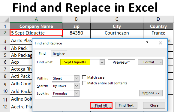
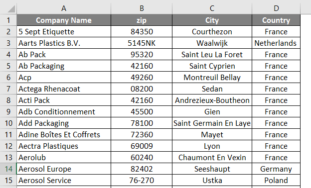
In this example, let’s see how can you use find and replace options. Some company details with the address in the spreadsheet are given below.

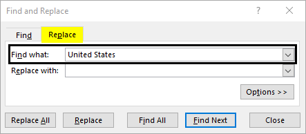
Open the spreadsheet where you want to find the word. The next step is to open the find option using the keyboard short cut Ctrl+F.

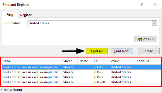
This will open a box where you can give the word that you want to find. After typing or pasting the word in the ‘Find What:’ area, Click on the ‘Find All’ button.

This will give you a list of places where ever the particular word is located. The first will be automatically selected, and the cell will be selected.

By clicking the ‘Find Next button, the cell selection will be moved to the second location, which is listed in the window.

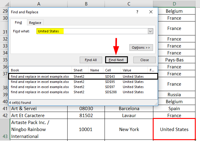
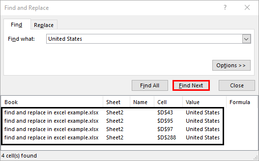
The ‘Find Next’ button will move the selection to the next corresponding locations. Until the list completes the search, it will change and show the different locations by selecting the corresponding cell. Once the list gets completed, it again moves to the first listed location.

Example #2 – Finding and Replacing a Word within Excel

In the above example, you were able to find a word within the given spreadsheet. Now let’s see how can you replace the word after finding it with another word or data. You may come across the situation to make changes to your data within a spreadsheet. If this is a continuous process, you want to replace a particular data where ever it appears in the spreadsheet.

Finding each data one by one and replacing, in the same way, is time-consuming. Here we can use the find and replace option in excel.

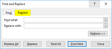
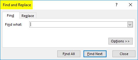
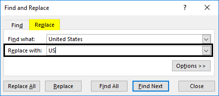
By pressing the shortcut keys in the keyboard Ctrl+H, a dialog box will get open. This will offer you two dialog boxes where you can provide the text you want to find and replace it with.

To Replace the given data Two options are available.

Replace
Replace All

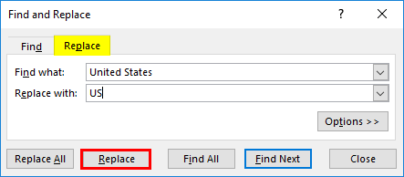
The ‘Replace’ button will work similarly to the ‘Find Next’ button. This will replace the given data one by one. Similar to the ‘Find Next’ button Replace will replace the data one by another.
Click on the ‘Replace All’ button the data will replace with the data mentioned in the ‘Replace With’ input textbox in a single click.

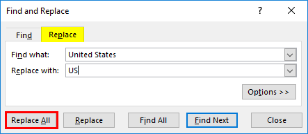
As a final result, this will show a dialog box with a number of replacements made in the entire spreadsheet. This message will help you to verify your data replacement among the worksheet.

Example #3 – Find and Replace with More Options

For the advanced find and replace, you have more options. This will provide you with more ways to specify the data that you need to find and replace. By customizing the data finding needs, you can make the find and replace it more effective within the spreadsheet.

Use the Ctrl+F shortcut to find the data. Once the find and replace window appears, click on the ‘Options’ button within the dialog box.

From the available option, you can select different options to find the data. There exists an option to select where you want to find the specified data from the dropbox near the ‘Within’ option; select one from the list, whether you want to find the data in a sheet or entire workbook.

Another option is to arrange your search. By row or column, you can perform the search. If you want to find data within different columns or row separately, this facility is better.

You can direct where you want to ‘Look in’ the mentioned data. The drop-down provides a list that contains the below options.

Formulas
Values
Comments

The selection will search the data in different areas instead of finding it all over the spreadsheet.

The different match cases are able to mention while finding the data. The two checkboxes are provided:

Match Case
Match entire cell contents

Match Case: This will find similar to the mentioned data. And any matching case will be highlighted.

Match Entire Cell Contents: Xerox copy of data will find. Similarities won’t be accepted while searching.

All these advanced search options are available to find and replace too. To find and replace within a special data format is another available customization.

The format dropdown will provide a new window where you can select the format of the data.

What is Find and Replace and How to Use it?

Find and replace is used to find data among a spreadsheet or worksheet. Find and replace is used as a combination. You can find data and replace the data with another mentioned data, which this facility uses in two ways.

Find
Find and Replace

From the ‘Home’ menu, select the ‘Find & Select’, which categorized under editing tools. A drop down will provide the find option and replace option.

Click on anyone, and a dialog box will be appeared to get the data you need to find.

Shortcut for Find and Replace

Instead of moving to all these, use the keyboard shortcut as below.

Find: Ctrl+F
Replace: Ctrl+H

Things to Remember

Advanced options will provide more customization to find and replace.
If the worksheet is in protected mode, the replacement will not work. Excel will not allow editing operations.
To avoid unwanted replacement, go with format options while replacing.
If the mentioned data to find within the spreadsheet does not exist, then excel will show a warning message “We couldn’t find the data looking for. Click options for more way to search”.

How to Search in Excel

Find and Replace in Excel allows you to quickly search all cells and formulas in a spreadsheet for all instances that match your search criteria. This guide will cover how to search in Excel and use find and replace in Excel.

Examples of what you might use the Excel Find function to search for:

All cells that contain the number “10”
All formulas that contain a reference to cell “B7”
All formulas with the SUM function

There are two ways to access the Excel Find function:

Press Ctrl + F
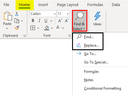
On the Home ribbon under “Find and Select” choose “Find”

To see a video tutorial of Go To Special check out our free Excel Crash Course.

Why use the Excel Find function?

There are many good reasons to use the Find function when performing financial modeling in Excel.

The main reason is to use it in conjunction with the Replace function, to quickly edit many cells and/or formulas at once.

For example, if you have hundreds of cells with formulas that link to a specific cell, you may want to use find and replace to change the formula. This will save you the pain of individually editing each cell with that formula, and guarantee that you don’t miss any.

For more time-saving tips, here is a list of all Excel shortcuts to speed up your modeling.

Example of Find and Replace in Excel

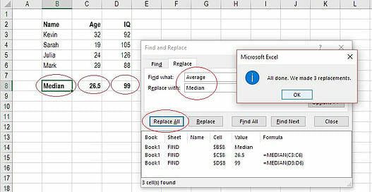
Below is an example of how to use Find and Replace to change the SUM formulas in the below table to all become MEDIAN formulas.

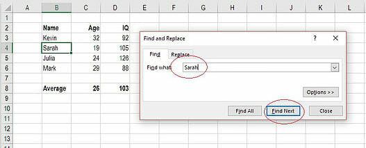
Part 1: Find a single data point

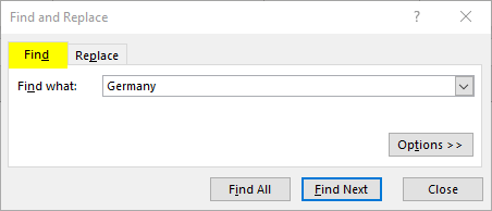
Press Ctrl + F
Type “Sarah”
Click Find Next

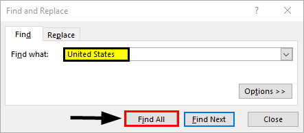
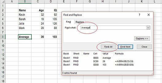
Part 2: Search in Excel all instances of something

Press Ctrl + F
Type “Average”
Click Find All

Part 3: Replace all instances of something

Press Ctrl + F
Click the “Replace” Tab to the top
Type “Average” in Find
Type “Median” in Replace
Click Replace All
Congratulations, all your SUM formulas are now MEDIAN formulas!

More Excel lessons

Thank you for reading CFI’s guide on how to search in Excel and how to find and replace in Excel.

If you want to master Excel please check out all CFI’s Excel Resources to learn all the most important formulas, functions, and shortcuts.

Additional CFI guides and resources you may find useful include:

Excel formulas and functions
Excel shortcuts
Go To Special
Index Match Match
See all Excel resources

Источник

Find

Replace

Find

Replace

Need more help?

Recommended articles

What is Find and Replace Feature in Excel?

Table of contents

How to Access the Find and Replace Feature of Excel?

Example #1–Find a Partial Match in a Worksheet

Example #2–Find a Partial Match in a Workbook

Example #3–Find an Exact Match in a Workbook

Example #4–Replace the Range Reference of a Formula

Example #5–Replace the Existing Text to Make Two Strings Identical

Example #6–Replace the Old Formatting of a Cell

Example #7–Find a Comment in a Worksheet

The Key Points Related to the Find and Replace Feature of Excel

Frequently Asked Questions

Recommended Articles

Line breaks for readability

More substitutions

Other uses

Introduction to Find and Replace in Excel

Examples of Find and Replace in Excel

Example #1- Finding a Word within Excel

Example #2 – Finding and Replacing a Word within Excel

Example #3 – Find and Replace with More Options

What is Find and Replace and How to Use it?

Things to Remember

Recommended Articles

How to Search in Excel

Why use the Excel Find function?

Example of Find and Replace in Excel

More Excel lessons