Find and replace excel что это - Word и Excel - помощь в работе с программами

На чтение 3 мин Опубликовано 21.08.2015

Найти
Заменить
Выделение группы ячеек

Вы можете использовать инструмент Find and Replace (Найти и заменить) в Excel, чтобы быстро найти нужный текст и заменить его другим текстом. Также вы можете использовать команду Go To Special (Выделение группы ячеек), чтобы быстро выделить все ячейки с формулами, комментариями, условным форматированием, константами и т.д.

Содержание

Найти
Заменить
Выделение группы ячеек

Найти

Чтобы быстро найти определенный текст, следуйте нашей инструкции:

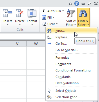
На вкладке Home (Главная) нажмите кнопку Find & Select (Найти и выделить) и выберите Find (Найти).

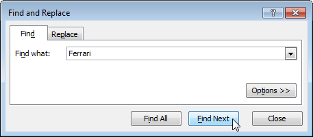
Появится диалоговое окно Find and Replace (Найти и заменить).
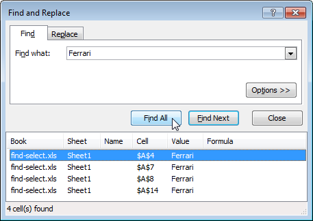
Введите текст, который требуется найти, к примеру, «Ferrari».
Нажмите кнопку Find Next (Найти далее).

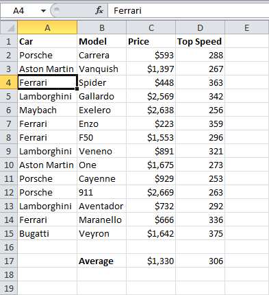
Excel выделит первое вхождение.
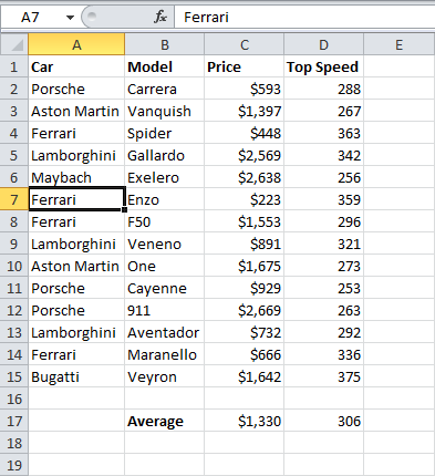
Нажмите кнопку Find Next (Найти далее) еще раз, чтобы выделить второе вхождение.
Чтобы получить список всех вхождений, кликните по Find All (Найти все).

Заменить

Чтобы быстро найти определенный текст и заменить его другим текстом, выполните следующие действия:

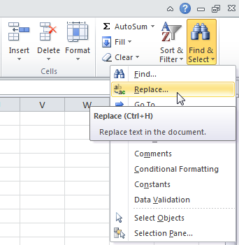
На вкладке Home (Главная) нажмите кнопку Find & Select (Найти и выделить) и выберите Replace (Заменить).

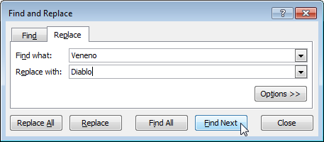
Появится одноимённое диалоговое окно с активной вкладкой Replace (Заменить).
Введите текст, который хотите найти (например, «Veneno») и текст, на который его нужно заменить (например, «Diablo»).
Кликните по Find Next (Найти далее).

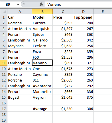
Excel выделит первое вхождение. Ещё не было сделано ни одной замены.
Нажмите кнопку Replace (Заменить), чтобы сделать одну замену.

Примечание: Используйте Replace All (Заменить все), чтобы заменить все вхождения.

Выделение группы ячеек

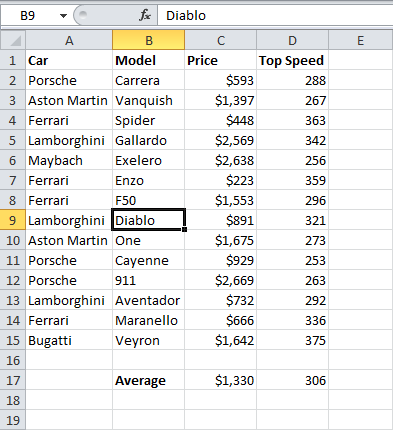
Вы можете воспользоваться инструментом Go To Special (Выделение группы ячеек), чтобы быстро выбрать все ячейки с формулами, комментарии, условным форматированием, константами и т.д. Например, чтобы выбрать все ячейки с формулами, сделайте следующее:

Выделите одну ячейку.
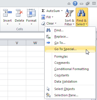
На вкладке Home (Главная) кликните по Find & Select (Найти и выделить) и выберите Go To Special (Выделение группы ячеек).

Примечание: Формулы, комментарии, условное форматирование, константы и проверка данных – все это можно найти с помощью команды Go To Special (Выделение группы ячеек).
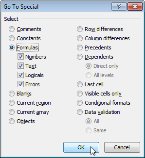
Поставьте галочку напротив Formulas (Формулы) и нажмите ОК.

Примечание: Вы можете искать ячейки с формулами, которые возвращают числа, текст, логические операторы (ИСТИНА и ЛОЖЬ) и ошибки. Также эти опции станут доступны, если вы отметите пункт Constants (Константы).

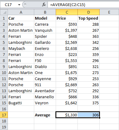
Excel выделит все ячейки с формулами:

Примечание: Если вы выделите одну ячейку, прежде чем нажать Find (Найти), Replace (Заменить) или Go To Special (Выделение группы ячеек), Excel будет просматривать весь лист. Для поиска в диапазоне ячеек, сначала выберите нужный диапазон.

Оцените качество статьи. Нам важно ваше мнение:

Источник

Use the Find and Replace features in Excel to search for something in your workbook, such as a particular number or text string. You can either locate the search item for reference, or you can replace it with something else. You can include wildcard characters such as question marks, tildes, and asterisks, or numbers in your search terms. You can search by rows and columns, search within comments or values, and search within worksheets or entire workbooks.

Find

To find something, press Ctrl+F, or go to Home > Editing > Find & Select > Find.

Note: In the following example, we’ve clicked the Options >> button to show the entire Find dialog. By default, it will display with Options hidden.

In the Find what: box, type the text or numbers you want to find, or click the arrow in the Find what: box, and then select a recent search item from the list.
Tips: You can use wildcard characters — question mark (?), asterisk (*), tilde (~) — in your search criteria.
- Use the question mark (?) to find any single character — for example, s?t finds «sat» and «set».
- Use the asterisk (*) to find any number of characters — for example, s*d finds «sad» and «started».
- Use the tilde (~) followed by ?, *, or ~ to find question marks, asterisks, or other tilde characters — for example, fy91~? finds «fy91?».
Click Find All or Find Next to run your search.

Tip: When you click Find All, every occurrence of the criteria that you are searching for will be listed, and clicking a specific occurrence in the list will select its cell. You can sort the results of a Find All search by clicking a column heading.
Click Options>> to further define your search if needed:
- Within: To search for data in a worksheet or in an entire workbook, select Sheet or Workbook.
- Search: You can choose to search either By Rows (default), or By Columns.
- Look in: To search for data with specific details, in the box, click Formulas, Values, Notes, or Comments.
  
  Note: Formulas, Values, Notes and Comments are only available on the Find tab; only Formulas are available on the Replace tab.
- Match case — Check this if you want to search for case-sensitive data.
- Match entire cell contents — Check this if you want to search for cells that contain just the characters that you typed in the Find what: box.
If you want to search for text or numbers with specific formatting, click Format, and then make your selections in the Find Format dialog box.

Tip: If you want to find cells that just match a specific format, you can delete any criteria in the Find what box, and then select a specific cell format as an example. Click the arrow next to Format, click Choose Format From Cell, and then click the cell that has the formatting that you want to search for.

Replace

To replace text or numbers, press Ctrl+H, or go to Home > Editing > Find & Select > Replace.

Note: In the following example, we’ve clicked the Options >> button to show the entire Find dialog. By default, it will display with Options hidden.

In the Find what: box, type the text or numbers you want to find, or click the arrow in the Find what: box, and then select a recent search item from the list.
Tips: You can use wildcard characters — question mark (?), asterisk (*), tilde (~) — in your search criteria.
- Use the question mark (?) to find any single character — for example, s?t finds «sat» and «set».
- Use the asterisk (*) to find any number of characters — for example, s*d finds «sad» and «started».
- Use the tilde (~) followed by ?, *, or ~ to find question marks, asterisks, or other tilde characters — for example, fy91~? finds «fy91?».
In the Replace with: box, enter the text or numbers you want to use to replace the search text.
Click Replace All or Replace.

Tip: When you click Replace All, every occurrence of the criteria that you are searching for will be replaced, while Replace will update one occurrence at a time.
Click Options>> to further define your search if needed:
- Within: To search for data in a worksheet or in an entire workbook, select Sheet or Workbook.
- Search: You can choose to search either By Rows (default), or By Columns.
- Look in: To search for data with specific details, in the box, click Formulas, Values, Notes, or Comments.
  
  Note: Formulas, Values, Notes and Comments are only available on the Find tab; only Formulas are available on the Replace tab.
- Match case — Check this if you want to search for case-sensitive data.
- Match entire cell contents — Check this if you want to search for cells that contain just the characters that you typed in the Find what: box.
If you want to search for text or numbers with specific formatting, click Format, and then make your selections in the Find Format dialog box.

Tip: If you want to find cells that just match a specific format, you can delete any criteria in the Find what box, and then select a specific cell format as an example. Click the arrow next to Format, click Choose Format From Cell, and then click the cell that has the formatting that you want to search for.

There are two distinct methods for finding or replacing text or numbers on the Mac. The first is to use the Find & Replace dialog. The second is to use the Search bar in the ribbon.

Find & Replace dialog

Search bar and options

Press Ctrl+F or go to Home > Find & Select > Find.
In Find what: type the text or numbers you want to find.
Select Find Next to run your search.
You can further define your search:
- Within: To search for data in a worksheet or in an entire workbook, select Sheet or Workbook.
- Search: You can choose to search either By Rows (default), or By Columns.
- Look in: To search for data with specific details, in the box, click Formulas, Values, Notes, or Comments.
- Match case — Check this if you want to search for case-sensitive data.
- Match entire cell contents — Check this if you want to search for cells that contain just the characters that you typed in the Find what: box.

Tips: You can use wildcard characters — question mark (?), asterisk (*), tilde (~) — in your search criteria.

Use the question mark (?) to find any single character — for example, s?t finds «sat» and «set».
Use the asterisk (*) to find any number of characters — for example, s*d finds «sad» and «started».
Use the tilde (~) followed by ?, *, or ~ to find question marks, asterisks, or other tilde characters — for example, fy91~? finds «fy91?».

Press Ctrl+F or go to Home > Find & Select > Find.
In Find what: type the text or numbers you want to find.
Select Find All to run your search for all occurrences.

Note: The dialog box expands to show a list of all the cells that contain the search term, and the total number of cells in which it appears.
Select any item in the list to highlight the corresponding cell in your worksheet.

Note: You can edit the contents of the highlighted cell.

Press Ctrl+H or go to Home > Find & Select > Replace.
In Find what, type the text or numbers you want to find.
You can further define your search:
- Within: To search for data in a worksheet or in an entire workbook, select Sheet or Workbook.
- Search: You can choose to search either By Rows (default), or By Columns.
- Match case — Check this if you want to search for case-sensitive data.
- Match entire cell contents — Check this if you want to search for cells that contain just the characters that you typed in the Find what: box.
  Tips: You can use wildcard characters — question mark (?), asterisk (*), tilde (~) — in your search criteria.
  - Use the question mark (?) to find any single character — for example, s?t finds «sat» and «set».
  - Use the asterisk (*) to find any number of characters — for example, s*d finds «sad» and «started».
  - Use the tilde (~) followed by ?, *, or ~ to find question marks, asterisks, or other tilde characters — for example, fy91~? finds «fy91?».
In the Replace with box, enter the text or numbers you want to use to replace the search text.
Select Replace or Replace All.
Tips:
- When you select Replace All, every occurrence of the criteria that you are searching for is replaced.
- When you select Replace, you can replace one instance at a time by selecting Next to highlight the next instance.

Select any cell to search the entire sheet or select a specific range of cells to search.
Press Command + F or select the magnifying glass to expand the Search bar and type the text or number you want to find in the search field.
Tips: You can use wildcard characters — question mark (?), asterisk (*), tilde (~) — in your search criteria.
- Use the question mark (?) to find any single character — for example, s?t finds «sat» and «set».
- Use the asterisk (*) to find any number of characters — for example, s*d finds «sad» and «started».
- Use the tilde (~) followed by ?, *, or ~ to find question marks, asterisks, or other tilde characters — for example, fy91~? finds «fy91?».
Press return.
Notes:
- To find the next instance of the item you are searching for, press return again or use the Find dialog box and select Find Next.
- To specify additional search options, select the magnifying glass and select Search in Sheet or Search in Workbook. You can also select the Advanced option, which launches the Find dialog.
Tip: You can cancel a search in progress by pressing ESC.

Find

To find something, press Ctrl+F, or go to Home > Editing > Find & Select > Find.

Note: In the following example, we’ve clicked > Search Options to show the entire Find dialog. By default, it will display with Search Options hidden.

In the Find what: box, type the text or numbers you want to find.
Tips: You can use wildcard characters — question mark (?), asterisk (*), tilde (~) — in your search criteria.
- Use the question mark (?) to find any single character — for example, s?t finds «sat» and «set».
- Use the asterisk (*) to find any number of characters — for example, s*d finds «sad» and «started».
- Use the tilde (~) followed by ?, *, or ~ to find question marks, asterisks, or other tilde characters — for example, fy91~? finds «fy91?».
Click Find Next or Find All to run your search.

Tip: When you click Find All, every occurrence of the criteria that you are searching for will be listed, and clicking a specific occurrence in the list will select its cell. You can sort the results of a Find All search by clicking a column heading.
Click > Search Options to further define your search if needed:
- Within: To search for data within a certain selection, choose Selection. To search for data in a worksheet or in an entire workbook, select Sheet or Workbook.
- Direction: You can choose to search either Down (default), or Up.
- Match case — Check this if you want to search for case-sensitive data.
- Match entire cell contents — Check this if you want to search for cells that contain just the characters that you typed in the Find what box.

Replace

To replace text or numbers, press Ctrl+H, or go to Home > Editing > Find & Select > Replace.

Note: In the following example, we’ve clicked > Search Options to show the entire Find dialog. By default, it will display with Search Options hidden.

In the Find what: box, type the text or numbers you want to find.
Tips: You can use wildcard characters — question mark (?), asterisk (*), tilde (~) — in your search criteria.
- Use the question mark (?) to find any single character — for example, s?t finds «sat» and «set».
- Use the asterisk (*) to find any number of characters — for example, s*d finds «sad» and «started».
- Use the tilde (~) followed by ?, *, or ~ to find question marks, asterisks, or other tilde characters — for example, fy91~? finds «fy91?».
In the Replace with: box, enter the text or numbers you want to use to replace the search text.
Click Replace or Replace All.

Tip: When you click Replace All, every occurrence of the criteria that you are searching for will be replaced, while Replace will update one occurrence at a time.
Click > Search Options to further define your search if needed:
- Within: To search for data within a certain selection, choose Selection. To search for data in a worksheet or in an entire workbook, select Sheet or Workbook.
- Direction: You can choose to search either Down (default), or Up.
- Match case — Check this if you want to search for case-sensitive data.
- Match entire cell contents — Check this if you want to search for cells that contain just the characters that you typed in the Find what box.

Need more help?

You can always ask an expert in the Excel Tech Community or get support in the Answers community.

What is Find and Replace Feature in Excel?

The Find and Replace feature of Excel looks for a data value and replaces it with another data value. This data value can be a text string, number, date or special character. The Find and Replace feature can search within a worksheet or workbook, by rows or columns, and within formulas, values or comments.

For example, in a financial report of Excel, the text string “asset” may need to be replaced with “assets.”

The purpose of using the Find and Replace feature in Excel is to locate certain information in a database. It also allows modifying the existing data values with a few clicks. By default, the Find and Replace excel feature looks for a partial match. But, it can also look for an exact match if the option “match entire cell contents” is selected.

What is Find and Replace Feature in Excel?
- How to Access the Find and Replace Feature of Excel?
  - Example #1–Find a Partial Match in a Worksheet
  - Example #2–Find a Partial Match in a Workbook
  - Example #3–Find an Exact Match in a Workbook
  - Example #4–Replace the Range Reference of a Formula
  - Example #5–Replace the Existing Text to Make Two Strings Identical
  - Example #6–Replace the Old Formatting of a Cell
  - Example #7–Find a Comment in a Worksheet
- The Key Points Related to the Find and Replace Feature of Excel
- Frequently Asked Questions
- Recommended Articles

How to Access the Find and Replace Feature of Excel?

The shortcuts to the Find and Replace excel feature are stated as follows:

“Ctrl+F” opens the Find tab of the Find and Replace feature.
“Ctrl+H” opens the Replace tab of the Find and Replace feature.

Alternatively, the “find” and “replace” options can be clicked from the “find & select” drop-down (“editing” group) of the Home tab. These options open the Find and Replace tabs of the Find and Replace feature of Excel.

Let us consider some examples to understand the working of the Find and Replace feature of Excel.

You can download this Find and Replace Excel Template here – Find and Replace Excel Template

Example #1–Find a Partial Match in a Worksheet

The following image shows two worksheets titled “Jan” and “Feb.” These worksheets contain datasets that report the sales made (column C) to different customers (column B) in January and February.

The names of the products, cost of goods sold (COGS), profits, and regions are also displayed in columns A, D, E, and F respectively. A similar dataset (with different numbers) is in columns H to M as well.

Find the name “Mitchel” in the worksheet “Jan.” Use the Find and Replace feature of Excel.

The steps to use find and replace function in excel is follows:

Go to the worksheet “Jan.” Next, press the keys “Ctrl+F” together. The Find tab of the “find and replace” dialog box opens. This is shown in the following image.
Note: By default, Excel searches in the currently active worksheet.
Type the word to be searched in the “find what” box. We type “Mitchel.”

Note that this search is not case-sensitive. So, even if the worksheet contains “MITCHEL,” it will show up in the search results.
Press either the “Enter” key or the “find next” option. The first occurrence of the name “Daniel Mitchel” is selected. So, cell B7 is selected, as shown in the following image. Clicking “find next” again and again selects the subsequent occurrences of “Mitchel.”
Notice that though we entered “Mitchel” in the “find what” box, Excel has selected the name “Daniel Mitchel.” This is called a partial match. It implies that if there are any additional words preceding or succeeding the search value, the entire string containing the search value is returned in the result.
Click “find all” to see all the strings containing “Mitchel.” The results are shown in the following image. These results display the following information:
• The column “book” displays the name of the workbook containing the search value.
• The column “sheet” displays the name of the worksheet containing the search value.
• The column “cell” displays the reference of the cells containing the search value.
• The column “value” displays the entire string containing the search value.

Notice that at the bottom of the dialog box, Excel displays the number of cells containing the search value. In this case, there are 8 cells in the worksheet “Jan,” which contain either “Mitchel” or “Daniel Mitchel.”

Difference between “find all” and “find next”: The “find all” option shows all the occurrences of the search value. Further, clicking any of the entries shown by this option takes the user to the corresponding cell.

The “find next” option helps scan through the different cells containing the search value. Clicking “find next” for the first time selects the first occurrence of the search value. Likewise, clicking “find next” the second time selects the second occurrence of the search value, and so on.

Example #2–Find a Partial Match in a Workbook

Working on the dataset of example #1, find the name “Mitchel” in the entire workbook. Use the Find and Replace feature of Excel.

The steps to search the stated string in the entire workbook are listed as follows:

Step 1: Press the keys “Ctrl+F” together. The Find tab of the “find and replace” window opens. Type the name “Mitchel” in the “find what” box.

Next, click “options,” shown within a black box in the following image.

Step 2: Clicking “options” expands the “find and replace” dialog box. Click the drop-down next to the option “within” and select “workbook.”

The selection is shown in the following image.

Step 3: Click “find all” to see all the results. The results are shown in the following image. This time the string “Mitchel” has been found in 16 cells of the workbook.

Clicking any of the entries will select the respective cell.

Example #3–Find an Exact Match in a Workbook

Working on the dataset of example #1, find an exact match of “Mitchel” in the entire workbook. Use the Find and Replace feature of Excel.

The steps to search the exact name in the entire workbook are listed as follows:

Step 1: Press the keys “Ctrl+F.” In the Find tab of the “find and replace” window, perform the following tasks:

Click “options” to expand the “find and replace” window.
Enter the name “Mitchel” in the “find what” box.
Select “workbook” in the box adjacent to “within.”
Select the checkbox of “match entire cell contents.”
Leave the “search” and “look in” parameters to default values which are “by rows” and “formulas” respectively.

The name of the “find what” box and the selections are shown in the following image.

Note: When the option “match entire cell contents” is selected, the Find and Replace excel feature looks for exactly those data values that have been entered in the “find what” box.

Step 2: Click “find all” to view all the exact matches of the name “Mitchel.” In the current workbook, 8 cells contain the exact name.

The results (shown in the following image) display the cell references, exact value, and the names of the worksheet and the workbook.

Example #4–Replace the Range Reference of a Formula

The following image shows the names (column A), salaries per annum (in $ in column B), salaries per month (in $ in column C), and departments (column D) of some employees of an organization.

The total salary per annum is shown in cell G3. This sum incorrectly considers the range B2:B10 in place of the range B2:B22. Rectify the range of the formulas in cells G3 and H3 so that the total salary per annum is calculated accurately. Use the Find and Replace feature of Excel.

The steps to edit a formula by using the Find and Replace feature of Excel are listed as follows:

Step 1: Copy the SUMThe SUM function in excel adds the numerical values in a range of cells. Being categorized under the Math and Trigonometry function, it is entered by typing “=SUM” followed by the values to be summed. The values supplied to the function can be numbers, cell references or ranges.read more formula of cell G3. For this, perform the given tasks:

Select cell G3. The formula [=SUM(B2:B10)] appears in the formula bar.
Copy this formula by pressing the keys “Ctrl+C” together.
Press the Escape (Esc) key once the formula has been copied. This will help exit the formula bar.

Alternatively, copy the formula of cell H3 by pressing the keys “Ctrl+C.” Next, press “Ctrl+H.”

Step 2: The Replace tab of the “find and replace” window opens. Paste the copied formula in the “find what” box, as shown in the following image. For pasting the formula, press the keys “Ctrl+V” together.

Note: Instead of copying and pasting, one can type the formula directly in the “find what” box.

Step 3: Enter the correct formula in the “replace with” box. So, type the formula “=SUM(B2:B22)” without the beginning and ending double quotation marks. This is shown in the following image.

Next, click “replace all.”

Step 4: Click “Ok” in the message stating the number of replacements made. The formulas of cells G3 and H3 change from “=SUM(B2:B10)” to “=SUM(B2:B22).” As a result, the total salary per annum changes.

The new output is shown within a red box in the following image. Hence, the total salary paid to the given 21 employees is $11,179,954 per annum.

Example #5–Replace the Existing Text to Make Two Strings Identical

There are two images titled “image 1” and “image 2.” Both images are in different worksheets. Further, the following information is given:

Image 1 shows the product code (column A) and prices (in $ in column B) of 21 products of a multinational organization.
Image 2 shows the product code (column A) and a blank column (column B) for the prices of the 21 products.

Notice that the product codes of both images consist of some letters prefixed to a number. The letters are different in both images, but the subsequent numbers are the same.

Make the product code identical in both images by using the Find and Replace feature of Excel. This will help fetch the prices of “image 1” in “image 2” (column B) with the VLOOKUP functionThe VLOOKUP excel function searches for a particular value and returns a corresponding match based on a unique identifier. A unique identifier is uniquely associated with all the records of the database. For instance, employee ID, student roll number, customer contact number, seller email address, etc., are unique identifiers.
read more.

Image 1

Image 2

The steps to make the product code identical by using the Find and Replace feature of Excel are listed as follows:

Step 1: Press the keys “Ctrl+H” to open the Replace tab of the “find and replace” window.

Step 2: Enter “pdc” in the “find what” box. Enter “prdct” in the “replace with” box. Next, click “replace all.” A message stating the number of replacements made is displayed. Click “Ok” to proceed.

The entries and the outputs are shown in the following image. Now, one can easily apply the VLOOKUP function to fetch the prices in this image. Had the replacements not been made, the VLOOKUP function could not have been applied.

Difference between “replace all” and “replace”: The “replace all” option replaces all the occurrences of the search value in one go. In contrast, the “replace” option replaces one occurrence at a time.

Therefore, use “replace” when not sure which occurrence needs to be replaced. Use “replace all” when all occurrences of the search value need to be replaced.

Example #6–Replace the Old Formatting of a Cell

The following image shows some departments of an organization. Cell A4 is in grey and cells B5, C2, and D5 are in blue. We want all the cells containing “marketing” to be in one color.

Therefore, replace the grey color of cell A4 with blue color. Use the Find and Replace feature of Excel.

The steps to change the formatting with the Find and Replace feature of Excel are listed as follows:

Step 1: Select the dataset whose formatting needs to be changed. We have selected the range A2:D6.

Next, press the keys “Ctrl+H” to open the Replace tab of the “find and replace” window. In this tab, click “options” shown on the right side.

This entire step is shown in the following image.

Step 2: Once “options” is clicked, the “find and replace” window expands. Click the drop-down arrow of the first “format” option (to the right of the “find what” box). Next, select “choose format from cell.”

The selection is shown within a black box in the following image.

Step 3: Select the cell whose formatting needs to be changed. We select cell A4. As a result, the “no format set” on the left of “format” changes to “preview.” This “preview” option reflects the color of cell A4, as shown in the following image.

Note: The “preview” option of the following image and cell A4 of the first image (at the beginning of this example) show a slight variation in color. Please ignore this variation, which may be due to different Excel versions being used to create images.

Step 4: Click the drop-down arrow of the second “format” option (to the right of the “replace with” box). Select “choose format from cell” and click any of the blue cells (B5, C2 or D5). Consequently, the “preview” option appears in blue, as shown in the following image.

Next, click “replace all.”

Step 5: Excel shows the number of replacements made. Click “Ok” to proceed. The output is shown in the following image.

Hence, cell A4 has also been colored blue. In this way, the formatting of a cell can be searched and replaced. So, we have searched for the grey color and replaced it with the blue color. Now, all cells containing “marketing” are in a single color.

Note: Alternatively, one can select the “format” option from both the “format” drop-downs. Thereafter, from the respective “fill” tabs, select the color to be searched and the color to be replaced with.

Example #7–Find a Comment in a Worksheet

The following image contains two datasets (range A1:D11 and range A13:D23) that show the gross sales (column B), cost of goods sold (COGS in column C), and profits (column D) of ten products of an organization. Further, the following information is given:

Both datasets pertain to different time periods. The figures in brackets in column D are the losses suffered by the organization.
In both datasets, each cell of column D contains commentsIn Excel, Insert Comment is a feature used to share tips or details with different users working within the same spreadsheet. You can either right-click on the required cell, click on “Insert Comment” & type the comment, use the shortcut key, i.e., Shift+F2, or click on the Review Tab & select “New Comment”. read more. This is indicated by the small, red triangles at the top-right side of each cell.
There are three kinds of comments, namely, “no commission,” “commission @ 5%,” and “commission @ 10%.”

Find the comment “no commission” in the current worksheet, which has been renamed “comment.” Use the Find and Replace feature of Excel.

The steps to search a specific comment by using the Find and Replace feature of Excel are listed as follows:

Step 1: Open the Find tab of the “find and replace” dialog box. For this, press the keys “Ctrl+F” together. Next, click “options.” Make the following selections in this window:

Select “sheet” and “by rows” in the “within” and “search” parameters. These are the default selections of Excel.
Select the option “comments” from the drop-down of “look in.”

The selection of the second pointer is shown within a black box in the following image.

Step 2: In the “find what” box, enter the string of the comment that needs to be searched. We have entered “no commission,” as shown in the following image.

Next, click “find all.”

Step 3: The search results are shown in the following image. Notice that 13 cells (refer to the bottom of the image) contain the comment “no commission.”

The references to cells containing the specific comment (no commission) are displayed in the column “cell.” The formulas (of column D) and the names of the workbook and worksheet are displayed in columns “formula,” “book,” and “sheet” respectively.

Clicking any of the entries of these results will select the cell containing the comment.

The Key Points Related to the Find and Replace Feature of Excel

The important points related to the Find and Replace feature of Excel are listed as follows:

The search can be limited to a specific range of the worksheet. For such restriction, select the range prior to opening the Find tab of the “find and replace” window. If no range is selected, Excel searches in the currently active sheet. If the search value cannot be found in the selected range or the active worksheet, a message stating the same is displayed.
The replacements can also be restricted to a specific region of the worksheet. For this, select the area (or range) prior to opening the Replace tab of the “find and replace” window. If no range is selected, Excel makes the replacements in the entire active sheet.
The Find and Replace excel feature can replace the existing formatting of cells with the new formatting. For this, make use of the two “format” drop-downs of the Replace tab.
The search value can be looked up in a protected worksheet, but a replacement cannot be made. For replacing, unprotect the sheet first.

Frequently Asked Questions

1. Define the Find and Replace feature and state how it is used in Excel.

The Find and Replace feature of Excel helps search a data value and replace it with another data value. The need to search a data value arises when certain information is to be located in a database. The need to replace a data value arises when the existing information requires to be changed.

The Find and Replace feature (or window) of Excel can be used in either of the following ways:

• Use the Find tab when a data value needs to be searched. Specify the data value in the “find what” box and click “find next” or “find all” to search.
• Use the Replace tab when one data value needs to be replaced by another. Specify the value to search and the value to replace with, in the “find what” and “replace with” boxes respectively. Click “replace” or “replace all” to make the replacements.

Note: Click the “options” button to view more features of the “find and replace” window of Excel.

2. How to use the Find and Replace feature with wildcards in Excel?

The Find and Replace feature can be used with the wildcard characters like an asterisk (*), question mark (?), and tilde (~) in the following ways:

• The asterisk looks for any number of characters. For instance, “ro*” will find the strings rose, product, root, metro, rhinoceros, and so on. So, the words having “ro” anywhere in the string will be returned in the search results.
• The question mark looks for a single character of the string. For instance, “s?m” will find the strings simplicity, sampling, similarity, blossom, troublesome, and so on. So, the words having any character between “s” and “m” (placed anywhere in the string) are returned in the search results.
• The tilde looks for the actual asterisk, question mark or tilde in the strings. For instance, “~?” will find “happy?,” “mer?ry,” “?joyful,” “cheerful?”, and so on. So, the words having a question mark anywhere in the string are returned in the search results. Likewise, “~*” and “~~” look for words that contain asterisk or tilde at any place in the string.

The wildcard characters stated in the preceding pointers [like “ro*,” “s?m,” “~?,” “~*,” or “~~”] need to be typed in the “find what” box. The value to be replaced with needs to be entered in the “replace with” box.

Note: To look for an exact match, select the option “match entire cell contents.”

3. How is the Find and Replace feature used for the following tasks of Excel?

1. Replace a value with nothing
2. Assign a format to specific cells

1. The steps to replace a value with nothing are listed as follows:

a. Open the Replace tab by pressing the keys “Ctrl+H.”
b. Type the value to be replaced with nothing in the “find what” box.
c. Leave the “replace with” box blank.
d. Click the “replace all” button.

All occurrences of the value typed in the “find what” box are deleted.

2. The steps to assign a format to specific cells are listed as follows:

a. Open the Replace tab by pressing the keys “Ctrl+H.”
b. In the “find what” box, type the text string to be formatted.
c. In the “replace with” box, type the same text string as that of the preceding step.
d. Click “options.” The “find and replace” window expands.
e. Click the “format” drop-down to the right of “replace with.” Select the option “format.” The “replace format” window opens.
f. Assign the desired formatting in the “alignment,” “font,” “border,” and “fill” tabs.
g. Click “Ok” in the “replace format” window. Click “replace all” in the “find and replace” window. Click “Ok ” in the message stating the number of replacements made.

The new formatting will be assigned to the cells containing the “find what” string. Notice that no replacements of data values will be made. This is because the text of “find what” and “replace with” boxes are the same. So, there is only a change in the formatting of specific cells.

Производить одновременный поиск в нескольких книгах

Найдите и замените во всех открытых файлах или только в выбранных книгах и листах.

Искать по всем или только по определенным типам данных

Вы можете искать значения, формулы, гиперссылки и комментарии одновременно или только в определенных типах данных.

Найти точные совпадения

Если частичное совпадение не подходит для ваших нужд, определите поиск, чтобы он соответствовал всему содержимому ячейки.

Выполнять поиск с учетом регистра

Если символы в нижнем и верхнем регистре имеют значение, установите флажок Учитывать регистр.

Заменить все или только выбранные результаты поиска

Можно заменить прямо в результатах поиска. Выберите все или некоторые из найденных элементов и нажмите «Заменить все».

Искать на активном листе или в выбранных ячейках

При необходимости уменьшите область поиска до текущего листа или выбранного диапазона ячеек.

Экспортировать найденные элементы в новую книгу

Выберите один из пяти вариантов экспорта: все найденные записи, строки или столбцы с найденными значениями и многое другое.

Найти и исправить опечатки

Оптимизируйте качество содержимого Excel, исключив все эти неприятные нечеткие совпадения и опечатки.

Приложение Ultimate Suite уже используют

Что такое расширенный поиск и замена в Excel?

Этот инструмент расширяет возможности стандартной функции «Найти и заменить» в Excel несколькими полезными особенностями:

Найти и заменить во всех открытых книгах или только на выбранных листах из разных книг.
Одновременный поиск значений, формул, гиперссылок и комментариев.
Экспорт найденных записей в новую книгу одним щелчком мыши.
И это еще не всё…

Могу ли я искать нужный мне текст в комментариях?

Да, вы можете искать любые символы в комментариях, просто выберите соответствующую опцию. Кроме того, вы можете просматривать формулы и даже гиперссылки.

Мне нужно найти и заменить определенное значение в нескольких книгах, возможно ли это?

Конечно! Самый простой способ — открыть все книги для поиска, а затем запустить расширенный поиск и замену. По умолчанию будут выбраны все листы во всех открытых книгах.

Может ли инструмент выполнять поиск только на определенных листах из разных книг?

Да. Когда вы запускаете надстройку, выбираются все листы из всех открытых книг, но вы можете отменить выбор тех из них, которые вам не нужны.

Если один и тот же текст написан как в верхнем, так и в нижнем регистре, могу ли я найти только прописные буквы?

Да. Чтобы выполнить поиск с учетом регистра, просто установите флажок « Учитывать регистр» .

Могу ли я заменить только часть найденных значений, а не все?

Конечно. Только вам решать, заменять ли все найденные записи, или только некоторые из них. Вы можете выбрать записи для замены на панели результатов поиска.

Мне нужно найти исключительно совпадения всего содержимого ячеек, возможно ли это?

Да. Чтобы найти только точные совпадения, выберите опцию Вся ячейка.

Как я могу экспортировать найденные данные?

По завершении поиска найденные записи отображаются на панели надстройки, и вы можете экспортировать их в новую книгу. Вы можете выбрать один из нескольких дополнительных параметров:

Экспортировать строки или столбцы с найденными значениями.
Экспортировать только выделенные записи, то есть элементы, которые вы сами выбрали в результатах поиска.
Экспортировать строки или столбцы, содержащие выделенные записи.

Могу ли я заменить все найденные записи в один клик?

Да, просто нажмите кнопку « Заменить все».

Могу ли я найти частичные совпадения в моем листе?

Да. Для этого используйте опцию поиска опечаток . Выберите диапазон, запустите утилиту, введите максимальное количество отличающихся символов и максимальное количество символов в слове или в ячейке. Нажмите кнопку Поиск опечаток . Вы увидите список всех значений, соответствующих вашим критериям поиска. Затем вы можете выбрать правильные значения и заменить ими неправильные.

Могу ли я выбирать просто выбрать найденные значения, не заменяя их?

Конечно. Кнопка Выбрать ячейки предлагает пять вариантов выбора:

строки со всеми найденными значениями.
столбцы со всеми найденными значениями.
выделенные записи целиком.
строки с выделенными записями.
столбцы с выделенными записями.

Скачать Ultimate Suite

Посмотреть все комментарии

Источник

How to Use Find and Replace in Excel: Full Guide (2023)

Find and Replace is one of the most common yet most resourceful features of Excel.

Searching through hundreds of thousands of rows is definitely not the best thing to do. And to replace something within these rows is even worse.

So Find and Replace lets you find a particular word or phrase in seconds regardless of the volume of the data.

It surely is one of the most needed functions of Excel. If you are yet to use this feature, jump right into the guide below to know all about it 🧐

You can also download our sample workbook for this article here if you want to practice along.

How to use Find and Replace

Using the Find and Replace feature is pretty simple. Press CTRL F to open the dialog box. Or select it from the Editing group.

Excel displays the find and replace options.

We have the following example data.

Example data set on the active worksheet.

Suppose we want to find Emily, the name of an employee working in a company. To do that, we will enter her name in the Find dialog box as:

Once you type the name, press Enter. Excel will highlight the cell containing the result.

Pro Tip!

Note that the name isn’t capitalized here. That’s because, in the find feature, capitalization doesn’t matter 😉

The Find Next button moves you to the next instance containing the search item by highlighting the cell.

The Find All button shows a list of all the occurrences where the search item occurs. Like this:

You can then choose whichever value you want, and it will direct you to the cell.

If you want to view all the cells at the same time, press CTRL A or manually select the entire list. Excel will highlight all the cells simultaneously:

Replace data with Find and Replace

Now, let’s see how the replace function works

Suppose we want to find the position of Accountant in this data. And replace it with Auditor.

To do this:

Select Replace tab from the Find and Replace dialog box. Or press CTRL H. You can also open it from the Find & Select option under the Editing group.

Enter the search term in the Find what box.
Type in the new term you want to replace the search term with.

Press Enter.

Note that we entered capitalized search terms. That’s because Replace needs to locate the exact text string. And then replace it with some other term.

Kasper Langmann, Microsoft Office Specialist

Similar to the Find feature in Excel, Replace tab also has the Replace Next and Replace all options.

The Replace Next option replaces each search term one by one.

The Replace next option only replaced one entry.

The Replace All replaces all the terms in one go. And displays a message confirming all the replacements have been made.

Excel makes all the replacements. question mark.

And that’s how you use the Find and Replace feature. Pretty easy, no? 😀

Advanced settings of Find and Replace

Now that you know all the basics of Find and Replace, let’s look at some advanced features it has to offer.

To open the advanced functions of the Find feature, click the Options button in the dialog box.

It displays a wide variety of options to choose from.

The option button shows a plethora of information.

Note that the list of options for the Find and Replace tab is the same. The only difference is that in Replace tab, you get an additional format option for the replace box.

Let’s study all these options in detail below.

Format: The format option lets you specify the format of the search item. Click the Format option at the top to select a format.

You can also choose the format for your text string from a particular cell. For that,

Click on the drop-down arrow next to Format.
Delete the existing format by clicking “Clear Find Format.”

Click “Choose Format From Cell”

The cursor appears with a dropper.

Just click on the cell whose format you want to copy, and click Replace all. The dialog box also shows a *Preview*.

Within: The within option lets you search a specific text string throughout the entire workbook 😵

So even if you don’t remember where a certain piece of text is in your workbook, you can simply search for it. This feature is actually very helpful when you have to search for a single term from extensive data.

Match Case: The match case option enables case sensitivity. This means that Excel will search for a specific term with the exact capitalization used.

Say we search “hr” in lowercase instead of uppercase and put a checkmark on the ‘Match Case’ option.

Press Find Next.

Excel will show a warning message because we didn’t capitalize the position properly.

If we write the same search term in uppercase, Excel searches and shows the result as:

Isn’t that amazing? 🤩

Search: The search option lets you select the order in which you want to search.

If you want to look for the search item row by row, select “by row”. And if you want to search column by column, select the “by column” option.

Match Entire Cell Contents: This option restricts Find and Replace to look only for characters you have entered in the box. If you even miss a period, Excel will show a warning message.

Say, we put a checkmark on the ‘Match entire cell contents‘ option. And type in the name “John,” whereas, in the data set, the correct name is “John O.”

This is what will happen:

And if we add “O.” to the same box, the result becomes:

Excel returns the correct result. This tool is great if your spreadsheet contains a large amount of data.

Look-in: The look-in option lets you specify the type of data of your search item.

The Find tab offers three types, namely, Formulas, Values, and comments. The Replace tab, on the other hand, uses only one type of data, i.e., Formulas.

If you only want to look for formulas, you can find them using the Go To Special option from Find & Select.

Go to Special to replace text and formulas

It offers a plethora of options and you can set the options as per your choice. You can use it to find other items too.

Formulas option similar to wildcard characters.

Just select the options and Excel will automatically apply them on your next search.

That’s it – Now what

And Tada! That’s how easy and fun it is to use Excel’s Find and Replace tools 🤗

Not only can you find and replace a particular text string in seconds, but you can also specify its format, location, order, and case sensitivity.

Undoubtedly, the Find and Replace feature of Excel is very powerful. But if you want to become an Excel master, there’s so much more you need to learn.

If you are new to this spreadsheet software, we suggest you begin learning Excel’s built-in functions; IF, SUMIF and VLOOKUP.

You can learn these superb functions for FREE in my 30-minute Excel course sent straight to your inbox.

Other resources

The Find and Replace feature in Excel is great. Especially when it comes to making tweaks and narrowing down your search criteria.

The function is easy to understand and use. But with a little more practice, you will be able to master this and make large-scale changes in your data in seconds.

If you like this article, we are sure you’d love to read more. Some related articles include the SEARCH, FIND, REPLACE and SUBSTITUTE functions in Excel.

Frequently asked questions

You can launch the Find and Replace dialog box by pressing CTRL + F.

Or you can find it in the Find & Select Menu under the Editing group from the Home Tab. If you want quick access to the Replace feature, you can use the keyboard shortcut CTRL + H.

If you prefer using formulas to find and replace items in Excel, you should try the SUBSTITUTE function. It is used when you know the exact characters of the text to be replaced. SUBSTITUTE function is a good alternative to Replace.

Kasper Langmann2023-01-19T12:05:02+00:00

Page load link

Источник

Найти

Заменить

Выделение группы ячеек

Find

Replace

Find

Replace

Need more help?

Recommended articles

What is Find and Replace Feature in Excel?

Table of contents

How to Access the Find and Replace Feature of Excel?

Example #1–Find a Partial Match in a Worksheet

Example #2–Find a Partial Match in a Workbook

Example #3–Find an Exact Match in a Workbook

Example #4–Replace the Range Reference of a Formula

Example #5–Replace the Existing Text to Make Two Strings Identical

Example #6–Replace the Old Formatting of a Cell

Example #7–Find a Comment in a Worksheet

The Key Points Related to the Find and Replace Feature of Excel

Frequently Asked Questions

Recommended Articles

Производить одновременный поиск в нескольких книгах

Искать по всем или только по определенным типам данных

Найти точные совпадения

Выполнять поиск с учетом регистра

Заменить все или только выбранные результаты поиска

Искать на активном листе или в выбранных ячейках

Экспортировать найденные элементы в новую книгу

Найти и исправить опечатки

Что такое расширенный поиск и замена в Excel?

Могу ли я искать нужный мне текст в комментариях?

Мне нужно найти и заменить определенное значение в нескольких книгах, возможно ли это?

Может ли инструмент выполнять поиск только на определенных листах из разных книг?

Если один и тот же текст написан как в верхнем, так и в нижнем регистре, могу ли я найти только прописные буквы?

Могу ли я заменить только часть найденных значений, а не все?

Мне нужно найти исключительно совпадения всего содержимого ячеек, возможно ли это?

Как я могу экспортировать найденные данные?

Могу ли я заменить все найденные записи в один клик?

Могу ли я найти частичные совпадения в моем листе?

Могу ли я выбирать просто выбрать найденные значения, не заменяя их?

How to Use Find and Replace in Excel: Full Guide (2023)

How to use Find and Replace

Replace data with Find and Replace

Advanced settings of Find and Replace

That’s it – Now what

Other resources

Frequently asked questions