
If the formulas are identical you can use Find and Replace with Match entire cell contents checked and Look in: Formulas. Select the range, go into Find and Replace, make your entries and `Replace All.

Or do you mean that there are several formulas with this same form, but different cell references? If so, then one way to go is a regular expression match and replace. Regular expressions are not built into Excel (or VBA), but can be accessed via Microsoft’s VBScript Regular Expressions library.
The following function provides the necessary match and replace capability. It can be used in a subroutine that would identify cells with formulas in the specified range and use the formulas as inputs to the function. For formulas strings that match the pattern you are looking for, the function will produce the replacement formula, which could then be written back to the worksheet.
Function RegexFormulaReplace(formula As String)
    Dim regex As New RegExp
    regex.Pattern = "=((([A-Z]+d+)-([A-Z]+d+))/([A-Z]+d+))"
'   Test if a match is found
    If regex.Test(formula) = True Then
        RegexFormulaReplace = regex.Replace(formula, "=(EXP((LN($1/$2)/14.32))-1")
    Else
        RegexFormulaReplace = CVErr(xlErrValue)
    End If
    Set regex = Nothing
End Function
In order for the function to work, you would need to add a reference to the Microsoft VBScript Regular Expressions 5.5 library. From the Developer tab of the main ribbon, select VBA and then References from the main toolbar. Scroll down to find the reference to the library and check the box next to it.

Use the Find and Replace features in Excel to search for something in your workbook, such as a particular number or text string. You can either locate the search item for reference, or you can replace it with something else. You can include wildcard characters such as question marks, tildes, and asterisks, or numbers in your search terms. You can search by rows and columns, search within comments or values, and search within worksheets or entire workbooks.

Find
To find something, press Ctrl+F, or go to Home > Editing > Find & Select > Find.
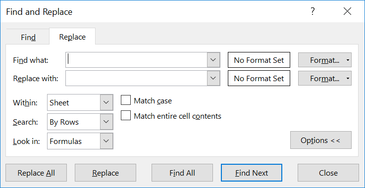
Note: In the following example, we’ve clicked the Options >> button to show the entire Find dialog. By default, it will display with Options hidden.

-
In the Find what: box, type the text or numbers you want to find, or click the arrow in the Find what: box, and then select a recent search item from the list.
Tips: You can use wildcard characters — question mark (?), asterisk (*), tilde (~) — in your search criteria.
-
Use the question mark (?) to find any single character — for example, s?t finds «sat» and «set».
-
Use the asterisk (*) to find any number of characters — for example, s*d finds «sad» and «started».
-
Use the tilde (~) followed by ?, *, or ~ to find question marks, asterisks, or other tilde characters — for example, fy91~? finds «fy91?».
-
-
Click Find All or Find Next to run your search.
Tip: When you click Find All, every occurrence of the criteria that you are searching for will be listed, and clicking a specific occurrence in the list will select its cell. You can sort the results of a Find All search by clicking a column heading.
-
Click Options>> to further define your search if needed:
-
Within: To search for data in a worksheet or in an entire workbook, select Sheet or Workbook.
-
Search: You can choose to search either By Rows (default), or By Columns.
-
Look in: To search for data with specific details, in the box, click Formulas, Values, Notes, or Comments.
Note: Formulas, Values, Notes and Comments are only available on the Find tab; only Formulas are available on the Replace tab.
-
Match case — Check this if you want to search for case-sensitive data.
-
Match entire cell contents — Check this if you want to search for cells that contain just the characters that you typed in the Find what: box.
-
-
If you want to search for text or numbers with specific formatting, click Format, and then make your selections in the Find Format dialog box.
Tip: If you want to find cells that just match a specific format, you can delete any criteria in the Find what box, and then select a specific cell format as an example. Click the arrow next to Format, click Choose Format From Cell, and then click the cell that has the formatting that you want to search for.
Replace
To replace text or numbers, press Ctrl+H, or go to Home > Editing > Find & Select > Replace.
Note: In the following example, we’ve clicked the Options >> button to show the entire Find dialog. By default, it will display with Options hidden.

-
In the Find what: box, type the text or numbers you want to find, or click the arrow in the Find what: box, and then select a recent search item from the list.
Tips: You can use wildcard characters — question mark (?), asterisk (*), tilde (~) — in your search criteria.
-
Use the question mark (?) to find any single character — for example, s?t finds «sat» and «set».
-
Use the asterisk (*) to find any number of characters — for example, s*d finds «sad» and «started».
-
Use the tilde (~) followed by ?, *, or ~ to find question marks, asterisks, or other tilde characters — for example, fy91~? finds «fy91?».
-
-
In the Replace with: box, enter the text or numbers you want to use to replace the search text.
-
Click Replace All or Replace.
Tip: When you click Replace All, every occurrence of the criteria that you are searching for will be replaced, while Replace will update one occurrence at a time.
-
Click Options>> to further define your search if needed:
-
Within: To search for data in a worksheet or in an entire workbook, select Sheet or Workbook.
-
Search: You can choose to search either By Rows (default), or By Columns.
-
Look in: To search for data with specific details, in the box, click Formulas, Values, Notes, or Comments.
Note: Formulas, Values, Notes and Comments are only available on the Find tab; only Formulas are available on the Replace tab.
-
Match case — Check this if you want to search for case-sensitive data.
-
Match entire cell contents — Check this if you want to search for cells that contain just the characters that you typed in the Find what: box.
-
-
If you want to search for text or numbers with specific formatting, click Format, and then make your selections in the Find Format dialog box.
Tip: If you want to find cells that just match a specific format, you can delete any criteria in the Find what box, and then select a specific cell format as an example. Click the arrow next to Format, click Choose Format From Cell, and then click the cell that has the formatting that you want to search for.
There are two distinct methods for finding or replacing text or numbers on the Mac. The first is to use the Find & Replace dialog. The second is to use the Search bar in the ribbon.
Find & Replace dialog
Search bar and options

-
Press Ctrl+F or go to Home > Find & Select > Find.
-
In Find what: type the text or numbers you want to find.
-
Select Find Next to run your search.
-
You can further define your search:
-
Within: To search for data in a worksheet or in an entire workbook, select Sheet or Workbook.
-
Search: You can choose to search either By Rows (default), or By Columns.
-
Look in: To search for data with specific details, in the box, click Formulas, Values, Notes, or Comments.
-
Match case — Check this if you want to search for case-sensitive data.
-
Match entire cell contents — Check this if you want to search for cells that contain just the characters that you typed in the Find what: box.
-
Tips: You can use wildcard characters — question mark (?), asterisk (*), tilde (~) — in your search criteria.
-
Use the question mark (?) to find any single character — for example, s?t finds «sat» and «set».
-
Use the asterisk (*) to find any number of characters — for example, s*d finds «sad» and «started».
-
Use the tilde (~) followed by ?, *, or ~ to find question marks, asterisks, or other tilde characters — for example, fy91~? finds «fy91?».

-
Press Ctrl+F or go to Home > Find & Select > Find.
-
In Find what: type the text or numbers you want to find.
-
Select Find All to run your search for all occurrences.

Note: The dialog box expands to show a list of all the cells that contain the search term, and the total number of cells in which it appears.
-
Select any item in the list to highlight the corresponding cell in your worksheet.
Note: You can edit the contents of the highlighted cell.

-
Press Ctrl+H or go to Home > Find & Select > Replace.
-
In Find what, type the text or numbers you want to find.
-
You can further define your search:
-
Within: To search for data in a worksheet or in an entire workbook, select Sheet or Workbook.
-
Search: You can choose to search either By Rows (default), or By Columns.
-
Match case — Check this if you want to search for case-sensitive data.
-
Match entire cell contents — Check this if you want to search for cells that contain just the characters that you typed in the Find what: box.
Tips: You can use wildcard characters — question mark (?), asterisk (*), tilde (~) — in your search criteria.
-
Use the question mark (?) to find any single character — for example, s?t finds «sat» and «set».
-
Use the asterisk (*) to find any number of characters — for example, s*d finds «sad» and «started».
-
Use the tilde (~) followed by ?, *, or ~ to find question marks, asterisks, or other tilde characters — for example, fy91~? finds «fy91?».
-
-
-
In the Replace with box, enter the text or numbers you want to use to replace the search text.
-
Select Replace or Replace All.
Tips:
-
When you select Replace All, every occurrence of the criteria that you are searching for is replaced.
-
When you select Replace, you can replace one instance at a time by selecting Next to highlight the next instance.
-
-
Select any cell to search the entire sheet or select a specific range of cells to search.
-
Press Command + F or select the magnifying glass to expand the Search bar and type the text or number you want to find in the search field.
Tips: You can use wildcard characters — question mark (?), asterisk (*), tilde (~) — in your search criteria.
-
Use the question mark (?) to find any single character — for example, s?t finds «sat» and «set».
-
Use the asterisk (*) to find any number of characters — for example, s*d finds «sad» and «started».
-
Use the tilde (~) followed by ?, *, or ~ to find question marks, asterisks, or other tilde characters — for example, fy91~? finds «fy91?».
-
-
Press return.
Notes:
-
To find the next instance of the item you are searching for, press return again or use the Find dialog box and select Find Next.
-
To specify additional search options, select the magnifying glass and select Search in Sheet or Search in Workbook. You can also select the Advanced option, which launches the Find dialog.
Tip: You can cancel a search in progress by pressing ESC.
-
Find
To find something, press Ctrl+F, or go to Home > Editing > Find & Select > Find.
Note: In the following example, we’ve clicked > Search Options to show the entire Find dialog. By default, it will display with Search Options hidden.

-
In the Find what: box, type the text or numbers you want to find.
Tips: You can use wildcard characters — question mark (?), asterisk (*), tilde (~) — in your search criteria.
-
Use the question mark (?) to find any single character — for example, s?t finds «sat» and «set».
-
Use the asterisk (*) to find any number of characters — for example, s*d finds «sad» and «started».
-
Use the tilde (~) followed by ?, *, or ~ to find question marks, asterisks, or other tilde characters — for example, fy91~? finds «fy91?».
-
-
Click Find Next or Find All to run your search.
Tip: When you click Find All, every occurrence of the criteria that you are searching for will be listed, and clicking a specific occurrence in the list will select its cell. You can sort the results of a Find All search by clicking a column heading.
-
Click > Search Options to further define your search if needed:
-
Within: To search for data within a certain selection, choose Selection. To search for data in a worksheet or in an entire workbook, select Sheet or Workbook.
-
Direction: You can choose to search either Down (default), or Up.
-
Match case — Check this if you want to search for case-sensitive data.
-
Match entire cell contents — Check this if you want to search for cells that contain just the characters that you typed in the Find what box.
-
Replace
To replace text or numbers, press Ctrl+H, or go to Home > Editing > Find & Select > Replace.
Note: In the following example, we’ve clicked > Search Options to show the entire Find dialog. By default, it will display with Search Options hidden.

-
In the Find what: box, type the text or numbers you want to find.
Tips: You can use wildcard characters — question mark (?), asterisk (*), tilde (~) — in your search criteria.
-
Use the question mark (?) to find any single character — for example, s?t finds «sat» and «set».
-
Use the asterisk (*) to find any number of characters — for example, s*d finds «sad» and «started».
-
Use the tilde (~) followed by ?, *, or ~ to find question marks, asterisks, or other tilde characters — for example, fy91~? finds «fy91?».
-
-
In the Replace with: box, enter the text or numbers you want to use to replace the search text.
-
Click Replace or Replace All.
Tip: When you click Replace All, every occurrence of the criteria that you are searching for will be replaced, while Replace will update one occurrence at a time.
-
Click > Search Options to further define your search if needed:
-
Within: To search for data within a certain selection, choose Selection. To search for data in a worksheet or in an entire workbook, select Sheet or Workbook.
-
Direction: You can choose to search either Down (default), or Up.
-
Match case — Check this if you want to search for case-sensitive data.
-
Match entire cell contents — Check this if you want to search for cells that contain just the characters that you typed in the Find what box.
-
Need more help?
You can always ask an expert in the Excel Tech Community or get support in the Answers community.
Recommended articles
Merge and unmerge cells
REPLACE, REPLACEB functions
Apply data validation to cells
Welcome Excellers to another #formulafriday blog post. Today let’s take a look at how to quickly change your Excel formula without having to rewrite any of those formulas. I have found this extremely useful when a request for a spreadsheet solution can suddenly change at the last minute from a user or even your boss. That is correct you can use Find and Replace to update a large number of Excel formulas with not a lot of effort.
Using Find And Replace – A Recap
First, let’s step this back to basics and look at the Find and Replace features in Excel. After all, you don’t want to be scrolling through hundreds if not thousands of Excel cells. Let’s start with how to find characters, text, numbers or dates in a range of cells, worksheet or the entire workbook.
- First, select or highlight the range of cells you want to search in. Alternatively, to search the whole worksheet simply select any cell in the active worksheet.
- Open the Find and Replace Dialog Box. Do this with Ctrl+F for the keyboard shortcut fans out there. Or you can hit Home Tab | Editing Group | Find And Select.
Next, in the Find What box, you need to enter the data you want to locate. You can choose at this stage to select (optional) the Options button to expand the dialog box and specify any desired options.
Within: Search just the current worksheet or the entire workbook.
Search: Select whether to search first across the rows or down the columns.
Look In: Select whether you want to search through the values or formula results, through the actual formulas, or if you want to look in the comments.
Match Case: Check this box if you want your search to be case-specific.
Match Entire Cell Contents: Check this box if you want your search results to list only the items that exactly match your search criteria.
- Click Find Next. Excel will find and jump to the first match of your search. If this is not the entry you’re looking for, click Find Next again. Excel advises you if it doesn’t locate the data you’re searching for.
Let’s Work Through An Example
So, now we have recapped how easy it is to use Find and Replace with Excel formulas. let’s get it working hard and update a spreadsheet with a lot of formulas that need changing. The example I am going to use is a worksheet which is recused every year. Everyone is happy with it and we do not need to redesign it every year. We do, however, have to update the formulas every year with Sales Targets from a different worksheet. That’s easy!.
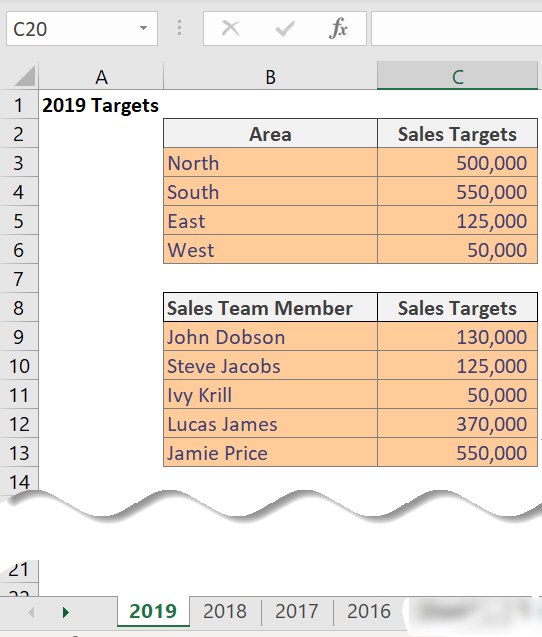
Here is a very small working example of this. I have sales targets for the North, South, East and West Regions. These are located in the following location ‘C:Sales’ in an Excel worksheet called ‘Sales Targets.xlsx’ Every year a new worksheet is added with the relevant year’s targets.
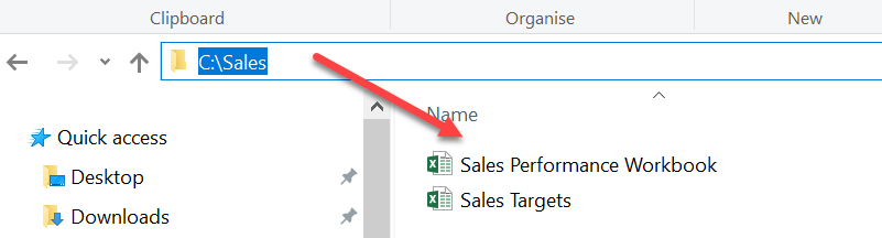
Also in this folder is the Sales Performance Workbook. This is linked to these Sales Target Figures. Here is how quick it is to update the formulas that still point to the 2018 targets to those of the 2019 targets.
Setting Up the Find And Replace For Excel Formulas
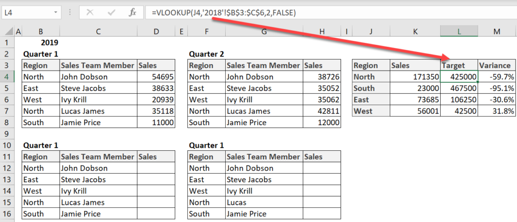
Select the cell range that you want to update. I have chosen the cell range L3: L7 in my Sales Performance Workbook. (I told you this was a very small example). Currently, the formula in this workbook is using the targets data from the worksheet named 2018 in the Sales Targets workbook.
I need this formula to point to the 2018 worksheet. So, first, we need to select the range of cells to update. Open the Find And Replace dialog box either with Ctrl+H shortcut or you can hit Home Tab | Editing Group | Find And Select.
In the Find box type the part of the Excel formula that you want to find. In this case, it is ‘2018’ and we then want to go ahead and replace it with ‘2019’

Now, if you have hundreds or even thousands of cell with Excel formulas to update then this is a really fast way to update formulas. I have used this to change SUM to AVERAGE, AVERAGE To MAX and MIN. In addition pointing formulas to differently workbooks or worksheet,ts as in this example.
What’s Next?
So, if you want more Excel and VBA tips then sign up for my Monthly Newsletter where I share 3 Tips on the first Wednesday of the month and receive my free Ebook, 30 Excel Tips.
If you want to see all of the blog posts in the Formula Friday series. Click on the link below
How To Excel At Excel – Formula Friday Blog Posts.


Watch Video – Useful Examples of Using Find & Replace in Excel
Last month, one of my colleagues got a data set in Excel, and he was banging his head to clean it. Since I was the only one in the office at that wee hour, he asked me if I could help. I used a simple technique using Find and Replace in Excel, and his data was all clean and polished. He thanked me, packed up, and left office.
He thanked me, packed up, and left office.
Excel Find and Replace feature is super powerful if you know how to best use it.
Using FIND and REPLACE in Excel (4 Examples)
Find and Replace in Excel can save a lot of time, and that is what matters most these days.
In this blog, I will share 4 amazing tips that I have shared with hundreds of my colleagues in my office. The response is always the same – “I wish I knew this earlier. It could have saved me so much of hard labor”.
#1 To Change Cell References Using Excel Find and Replace
Sometimes when you work with a lot of formulas, there is a need to change a cell reference in all the formulas. It could take you a lot of time if you manually change it in every cell that has a formula.
Here is where Excel Find and Replace comes in handy. It can easily find a cell reference in all the formulas in the worksheet (or in the selected cells) and replace it with another cell reference.
For example, suppose you have a huge dataset with formula in that uses $A$1 as one of the cell references (as shown below). If you need to change $A$1 with $B$1, you can do that using Find and Replace in Excel.

Here are the steps to do this:
- Select the cells that have the formula in which you want to replace the reference. If you want to replace in the entire worksheet, select the entire worksheet.
- Go to Home –> Find and Select –> Replace (Keyboard Shortcut – Control + H).
- In the Find and Replace dialogue box, use the following details:
- Find what: $A$1 (the cell reference you want to change).
- Replace with: $B$1 (the new cell reference).

- Click on Replace All.


This would instantly update all the formulas with the new cell reference.
Note that this would change all the instances of that reference. For example, if you have the reference $A$1 two times in a formula, both the instances would be replaced by $B$1.
#2 To Find and Replace Formatting in Excel
This is a cool feature when you want to replace existing formatting with some other formatting. For example, you may have cells with an orange background color and you want to change all these cell’s background color to red. Instead of manually doing this, use Find and Replace to do this all at once.
Here are the steps to do this:
- Select the cells for which you want to find and replace the formatting. If you want to find and replace a specific format in the entire worksheet, select the entire worksheet.
- Go to Home –> Find and Select –> Replace (Keyboard Shortcut – Control + H).
- Click on the Options button. This will expand the dialogue box and show you more options.

- Click on the Find what Format button. It will show a drop-down with two options – Format and Choose Format from Cell.
- Now you need to specify the format that you want instead of the one selected in the previous step. Click on the Replace with Format button. It will show a drop-down with two options – Format and Choose Format from Cell.
- Click on the Replace All button.

You can use this technique to replace a lot of things in formatting. It can pick up and replace formats such as background color, borders, font type/size/color, and even merged cells.
#3 To Add or Remove Line Break
What do you do when you have to go to a new line in an Excel cell.
You press Alt + Enter.
And what do you do when you want to revert this?
You delete it manually.. isn’t it?
Imagine you have hundreds of line breaks that you want to delete. removing line breaks manually can take a lot of time.
Here is the good news, you don’t need to do this manually. Excel Find and Replace has a cool trick up its sleeves that will make it happen in a snap.
Here are the steps to remove all the line breaks at once:
- Select the data from which you want to remove the line breaks.
- Go to Home –> Find and Select –> Replace (Keyboard Shortcut – Control + H).

- In the Find and Replace Dialogue Box:
- Find What: Press Control + J (you may not see anything except for a blinking dot).
- Replace With: Space bar character (hit space bar once).

- Click on Replace All.


And Woosh! It would magically remove all the line breaks from your worksheet.
#4 To Remove Text Using Wildcard Characters
This one saved me hours. I got a list as shown below, and I had to remove the text between parenthesis.

If you have a huge data-set, removing the parenthesis and the text between it can take you hours. But Find and Replace in Excel can do this in less than 10 seconds.
- Select the data
- Go to Home –> Find and Select –> Replace (Keyboard Shortcut – Control + H)
- In the Find and Replace Dialogue Box:
- Find What: (*)
Note I have used an asterisk, which is a wildcard character that represents any number of characters. - Replace With: Leave this Blank.

- Find What: (*)

I hope you find these tips helpful. If there are any other tricks that helped you save time, do share it with us!!
You May Also Like the Following Excel Tips & Tutorials:
- 24 Excel Tricks to Make You Sail through Day-to-day work.
- 10 Super Neat Ways to Clean Data in Excel Spreadsheets.
- 10 Excel Data Entry Tips You Can’t Afford to Miss.
- Suffering from Slow Excel Spreadsheets? Try these 10 Speed-up Tips.
- How to Filter Cells with Bold Font Formatting in Excel.
- How to Transpose Data in Excel.
This post will guide you how to replace formulas with their calculated values in Excel. How do I replace all formulas with their values using VBA Macro in Excel.
- Replace Formulas with Their Values
- Replace Formulas with Their Values Using VBA
Assuming that you have a list of data that contain formulas in range B1:B4, and you want to replace all formulas with their calculated values, how to do it. You can use the Paste Special command or an Excel VBA Macro to achieve the result.
If you want to replace all formulas in the selected range of cells with their values in Excel, you can do the following steps:
#1 select the range of cells that contain formulas. And press Ctrl + C keys on your keyboard.
#2 right click on the selected cells, and select the Paste Values menu under the Paste Options from the popup menu list.
#3 you would notice that all the formulas have been replaced with their calculated results in the selected range.
Replace Formulas with Their Values Using VBA
You can also use an Excel VBA Macro to achieve the same result of replacing all formulas with their calculated values. Just do the following steps:
#1 open your excel workbook and then click on “Visual Basic” command under DEVELOPER Tab, or just press “ALT+F11” shortcut.

#2 then the “Visual Basic Editor” window will appear.
#3 click “Insert” ->”Module” to create a new module.

#4 paste the below VBA code into the code window. Then clicking “Save” button.
#5 back to the current worksheet, then run the above excel macro. Click Run button.
#6 Please select one range that contain formuals. Click OK button.
#7 Let’s see the result: