
So, there are times when you would like to know that a value is in a list or not. We have done this using VLOOKUP. But we can do the same thing using COUNTIF function too. So in this article, we will learn how to check if a values is in a list or not using various ways.
Check If Value In Range Using COUNTIF Function
So as we know, using COUNTIF function in excel we can know how many times a specific value occurs in a range. So if we count for a specific value in a range and its greater than zero, it would mean that it is in the range. Isn’t it?
Generic Formula
=COUNTIF(range,value)>0
Range: The range in which you want to check if the value exist in range or not.
Value: The value that you want to check in the range.
Let’s see an example:
Excel Find Value is in Range Example
For this example, we have below sample data. We need a check-in the cell D2, if the given item in C2 exists in range A2:A9 or say item list. If it’s there then, print TRUE else FALSE.
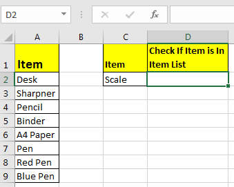
Write this formula in cell D2:
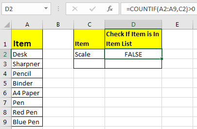
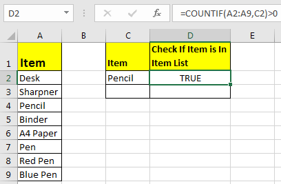
Since C2 contains “scale” and it’s not in the item list, it shows FALSE. Exactly as we wanted. Now if you replace “scale” with “Pencil” in the formula above, it’ll show TRUE.
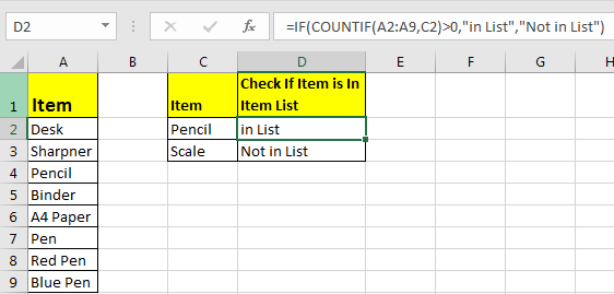
Now, this TRUE and FALSE looks very back and white. How about customizing the output. I mean, how about we show, “found” or “not found” when value is in list and when it is not respectively.
Since this test gives us TRUE and FALSE, we can use it with IF function of excel.
Write this formula:
=IF(COUNTIF(A2:A9,C2)>0,»in List»,»Not in List»)
You will have this as your output.
What If you remove “>0” from this if formula?
=IF(COUNTIF(A2:A9,C2),»in List»,»Not in List»)
It will work fine. You will have same result as above. Why? Because IF function in excel treats any value greater than 0 as TRUE.
How to check if a value is in Range with Wild Card Operators
Sometimes you would want to know if there is any match of your item in the list or not. I mean when you don’t want an exact match but any match.
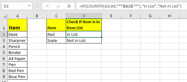
For example, if in the above-given list, you want to check if there is anything with “red”. To do so, write this formula.
=IF(COUNTIF(A2:A9,»*red*»),»in List»,»Not in List»)
This will return a TRUE since we have “red pen” in our list. If you replace red with pink it will return FALSE. Try it.
Now here I have hardcoded the value in list but if your value is in a cell, say in our favourite cell B2 then write this formula.
IF(COUNTIF(A2:A9,»*»&B2&»*»),»in List»,»Not in List»)
There’s one more way to do the same. We can use the MATCH function in excel to check if the column contains a value. Let’s see how.
Find if a Value is in a List Using MATCH Function
So as we all know that MATCH function in excel returns the index of a value if found, else returns #N/A error. So we can use the ISNUMBER to check if the function returns a number.
If it returns a number ISNUMBER will show TRUE, which means it’s found else FALSE, and you know what that means.
Write this formula in cell C2:
=ISNUMBER(MATCH(C2,A2:A9,0))
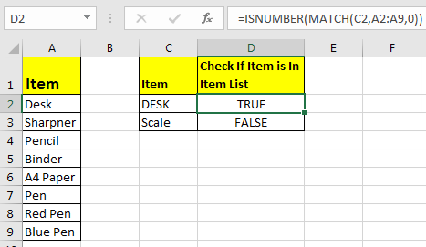
The MATCH function looks for an exact match of value in cell C2 in range A2:A9. Since DESK is on the list, it shows a TRUE value and FALSE for SCALE.
So yeah, these are the ways, using which you can find if a value is in the list or not and then take action on them as you like using IF function. I explained how to find value in a range in the best way possible. Let me know if you have any thoughts. The comments section is all yours.
Related Articles:
How to Check If Cell Contains Specific Text in Excel
How to Check A list of Texts In String in Excel
How to take the Average Difference between lists in Excel
How to Get Every Nth Value From A list in Excel
Popular Articles:
50 Excel Shortcuts to Increase Your Productivity
How to use the VLOOKUP Function in Excel
How to use the COUNTIF function in Excel
How to use the SUMIF Function in Excel
What is Find and Select Tool In Excel?
The Find and Select in Excel tool are useful for finding data as required. Along with the FIND function, the Replace function in excelThe Replace function is a text function that replaces an old string with a new one. The input required is the old text, new text, and the starting and ending numbers of the characters that need to be replaced.read more is also handy, which helps find the specific text and replace it with other text(s).
You can download this Find Excel Template here – Find Excel Template
Table of contents
- What is Find and Select Tool In Excel?
- How to use Find and Select in Excel?
- Things to remember
- Recommended Articles
How to use Find and Select in Excel?
Let us follow the below steps:
- First, under the Home tab is the Find Select Excel section.

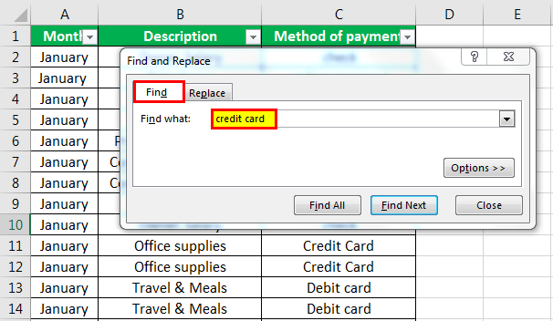
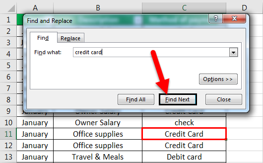
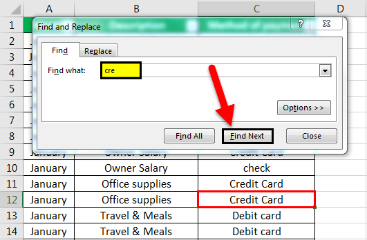
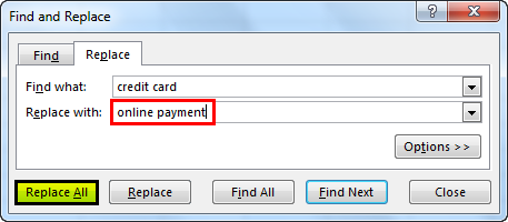
- Suppose we want to find a credit card from the data given. First, we need to go to the Find section and type credit card.

- When we press Find Next, we get the following result where there is a credit card.

- The find also works with fuzzy logic. For example, suppose we give cre in the find section. It will find the relevant words that contain cre.

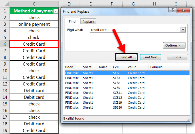
- To find the given text in all places of the worksheet, click Find All. As a result, it will highlight the keyword present everywhere in the worksheet.

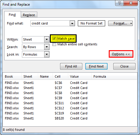
- We can match cases also within the worksheet to find case search sensitive data. First, we must click on Options, then select the Match case option.

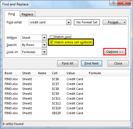
- To find cells containing just the characters typed in the Find what box, we must select the Match entire cell contents checkbox.
- We can also find it through an excel keyboard shortcut. First, we need to press CTRL + F and then the Find Replace tab will appear.

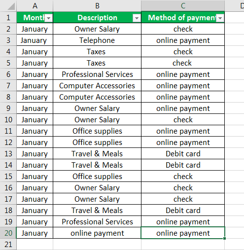
- If we want to replace something, we can use the Replace tab. For example, we want to replace credit with online payment. Then, we must click Replace All.

- As a result, it will replace all the cells containing credit with online payment.

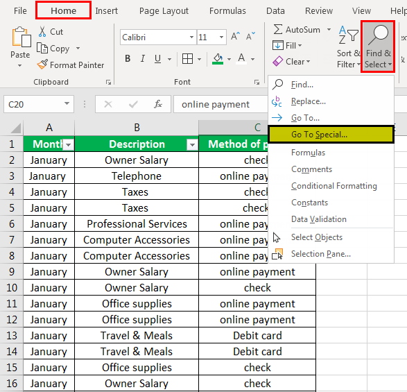
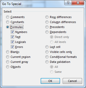
- Then, we must go to Excel’s Go to Special feature.

- This feature can quickly select all that contains formulas, conditional formatting, constant, data validation, etc.


Things to remember
- Excel saves formatting that is defined. If one searches the worksheet for data again and cannot find the characters, they must clear the formatting options from the previous search.
- In the above case, first, we need to go to the “Find and Replace” dialog box, click the “Find” tab, and click “Options” to display options for formatting. Then, we must click the arrow next to “Format” and click “Clear Find Format.”
- There is no option to replace the value in a cell comment.
Recommended Articles
This article is a guide to Find and Select in Excel. We discuss using Excel Find and Select tool and an example and downloadable template here. You may also look at these useful functions in Excel: –
- Apply Conditional Formatting for Dates
- How to Find Duplicates in Excel?
- Find and Replace in Excel
- Fill Down in Excel
Reader Interactions
This will return the matching word or an error if no match is found. For this example I used the following.
List of words to search for: G1:G7
Cell to search in: A1
=INDEX(G1:G7,MAX(IF(ISERROR(FIND(G1:G7,A1)),-1,1)*(ROW(G1:G7)-ROW(G1)+1)))
Enter as an array formula by pressing Ctrl+Shift+Enter.
This formula works by first looking through the list of words to find matches, then recording the position of the word in the list as a positive value if it is found or as a negative value if it is not found. The largest value from this array is the position of the found word in the list. If no word is found, a negative value is passed into the INDEX() function, throwing an error.
To return the row number of a matching word, you can use the following:
=MAX(IF(ISERROR(FIND(G1:G7,A1)),-1,1)*ROW(G1:G7))
This also must be entered as an array formula by pressing Ctrl+Shift+Enter. It will return -1 if no match is found.
Look up values in a list of data
Excel for Microsoft 365 Excel for the web Excel 2021 Excel 2019 Excel 2016 Excel 2013 Excel 2010 Excel 2007 More…Less
Let’s say that you want to look up an employee’s phone extension by using their badge number, or the correct rate of a commission for a sales amount. You look up data to quickly and efficiently find specific data in a list and to automatically verify that you are using correct data. After you look up the data, you can perform calculations or display results with the values returned. There are several ways to look up values in a list of data and to display the results.
What do you want to do?
-
Look up values vertically in a list by using an exact match
-
Look up values vertically in a list by using an approximate match
-
Look up values vertically in a list of unknown size by using an exact match
-
Look up values horizontally in a list by using an exact match
-
Look up values horizontally in a list by using an approximate match
-
Create a lookup formula with the Lookup Wizard (Excel 2007 only)
Look up values vertically in a list by using an exact match
To do this task, you can use the VLOOKUP function, or a combination of the INDEX and MATCH functions.
VLOOKUP examples

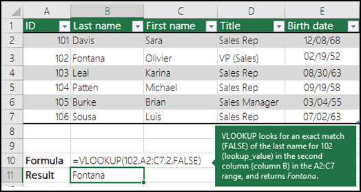
For more information, see VLOOKUP function.
INDEX and MATCH examples
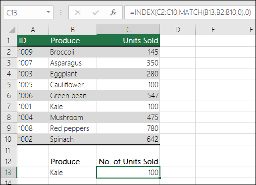
In simple English it means:
=INDEX(I want the return value from C2:C10, that will MATCH(Kale, which is somewhere in the B2:B10 array, where the return value is the first value corresponding to Kale))
The formula looks for the first value in C2:C10 that corresponds to Kale (in B7) and returns the value in C7 (100), which is the first value that matches Kale.
For more information, see INDEX function and MATCH function.
Top of Page
Look up values vertically in a list by using an approximate match
To do this, use the VLOOKUP function.
Important: Make sure the values in the first row have been sorted in an ascending order.
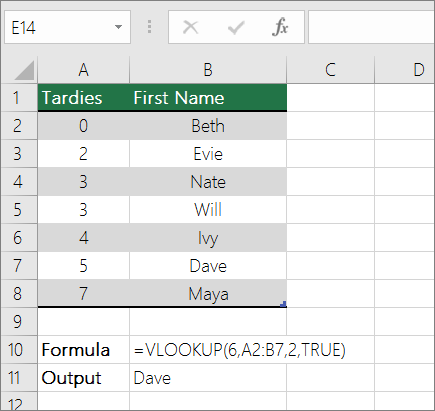
In the above example, VLOOKUP looks for the first name of the student who has 6 tardies in the A2:B7 range. There is no entry for 6 tardies in the table, so VLOOKUP looks for the next highest match lower than 6, and finds the value 5, associated to the first name Dave, and thus returns Dave.
For more information, see VLOOKUP function.
Top of Page
Look up values vertically in a list of unknown size by using an exact match
To do this task, use the OFFSET and MATCH functions.
Note: Use this approach when your data is in an external data range that you refresh each day. You know the price is in column B, but you don’t know how many rows of data the server will return, and the first column isn’t sorted alphabetically.
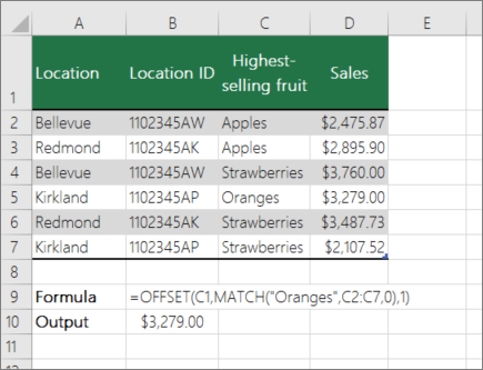
C1 is the upper left cells of the range (also called the starting cell).
MATCH(«Oranges»,C2:C7,0) looks for Oranges in the C2:C7 range. You should not include the starting cell in the range.
1 is the number of columns to the right of the starting cell where the return value should be from. In our example, the return value is from column D, Sales.
Top of Page
Look up values horizontally in a list by using an exact match
To do this task, use the HLOOKUP function. See an example below:
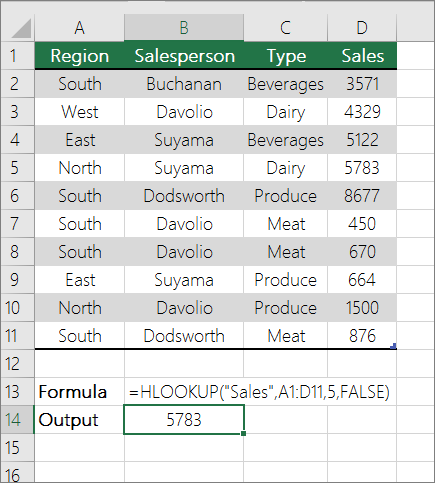
HLOOKUP looks up the Sales column, and returns the value from row 5 in the specified range.
For more information, see HLOOKUP function.
Top of Page
Look up values horizontally in a list by using an approximate match
To do this task, use the HLOOKUP function.
Important: Make sure the values in the first row have been sorted in an ascending order.
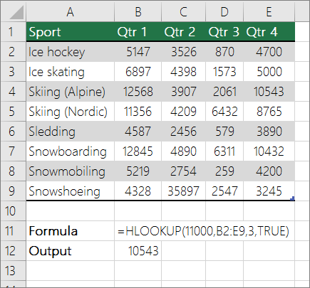
In the above example, HLOOKUP looks for the value 11000 in row 3 in the specified range. It does not find 11000 and hence looks for the next largest value less than 1100 and returns 10543.
For more information, see HLOOKUP function.
Top of Page
Create a lookup formula with the Lookup Wizard (Excel 2007 only)
Note: The Lookup Wizard add-in was discontinued in Excel 2010. This functionality has been replaced by the function wizard and the available Lookup and reference functions (reference).
In Excel 2007, the Lookup Wizard creates the lookup formula based on a worksheet data that has row and column labels. The Lookup Wizard helps you find other values in a row when you know the value in one column, and vice versa. The Lookup Wizard uses INDEX and MATCH in the formulas that it creates.
-
Click a cell in the range.
-
On the Formulas tab, in the Solutions group, click Lookup.
-
If the Lookup command is not available, then you need to load the Lookup Wizard add-in program.
How to load the Lookup Wizard Add-in program
-
Click the Microsoft Office Button
 , click Excel Options, and then click the Add-ins category.
 -
In the Manage box, click Excel Add-ins, and then click Go.
-
In the Add-Ins available dialog box, select the check box next to Lookup Wizard, and then click OK.
-
Follow the instructions in the wizard.
 , click Excel Options, and then click the Add-ins category.
Top of Page
Need more help?
Want more options?
Explore subscription benefits, browse training courses, learn how to secure your device, and more.
Communities help you ask and answer questions, give feedback, and hear from experts with rich knowledge.
A while back Vernon asked me how he could search one cell and compare it to a list of words. If any of the words in the list existed then return the matching word.
Ugh, I’ve written that 3 times and I’m not sure it’s any clearer…let’s look at an example.
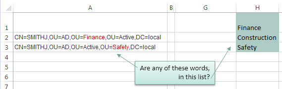
I’ve highlighted the matching words in column A red.
What we want Excel to do is to check the text string in column A to see if any of the words in our list in H1:H3 are present, if they are then return the matching word. Note: I’ve given cells H1:H3 the named range ‘list’.
There are a few ways we can tackle this so let’s take a look at our options.
Warning: this is quite an advanced topic which requires an array formula to solve it.
Update: It’s easier and more robust to use Power Query to search for text strings, including case and non-case sensitive searches.
Non-Case Sensitive Matching
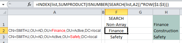
If you aren’t worried about case sensitive matches then you can use the SEARCH function with INDEX, SUMPRODUCT and ISNUMBER like this:
=INDEX(list,SUMPRODUCT(ISNUMBER(SEARCH(list,A2))*ROW($1:$3)))
In English our formula reads:
SEARCH cell A2 to see if it contains any words listed in cells H1:H3 (i.e. the named range ‘list’) and return the number of the character in cell A2 where the word starts. Our formula becomes:
=INDEX(list,SUMPRODUCT(ISNUMBER({20;#VALUE!;#VALUE!})*ROW($1:$3)))
i.e. in cell A2 the ‘F’ in the word ‘Finance’ starts in position 20.
Now using ISNUMBER test to see if the SEARCH formula returns any numbers (if it does it means there is a match). ISNUMBER will return TRUE if there is a number and FALSE if not (this gives us a list of Boolean TRUE or FALSE values). Our formula becomes:
=INDEX(list,SUMPRODUCT({TRUE;FALSE;FALSE}*ROW($1:$3)))
Use the ROW function to return an array of numbers {1;2;3} (see notes below on why I’ve used ROW in this formula). Our formula becomes:
=INDEX(list,SUMPRODUCT({TRUE;FALSE;FALSE}*{1;2;3}))
When you multiply Boolean TRUE/FALSE values they become their numeric equivalents i.e. TRUE = 1 and FALSE = 0. So our formula evaluates this ({TRUE;FALSE;FALSE}*{1;2;3}) like so: {1*1, 0*2, 0*3} and our formula becomes:
=INDEX(list,SUMPRODUCT({1;0;0}))
SUMPRODUCT simply sums the values {1+0+0} which gives us 1. Note: by using SUMPRODUCT we are avoiding the need for an array formula that requires CTRL+SHIFT+ENTER. Our formula becomes:
=INDEX(list,1)
Index can now go ahead and return the 1st value in the range of cells H1:H3 which is ‘Finance’.
Note: the above formula will not work if a match isn’t found. If you want to return an error if a match isn’t found then you can use this variation:
=INDEX(list,IF(SUMPRODUCT(--ISNUMBER(SEARCH(list,A2)))<>0,SUMPRODUCT(ISNUMBER(SEARCH(list,A2))*ROW($1:$3)),NA()))
Not as elegant, is it? In which case you might prefer one of the array formulas below.
Notes about the ROW Function:
The ROW function simply returns the row number of a reference. e.g. ROW(A2) would return 2. When used in an array formula it will return an array of numbers. e.g. ROW(A2:A4) will return {2;3;4}. We can also give just the row reference(s) to the ROW function like so ROW(2:4).
In this formula we have used ROW to simply return an array of values {1;2;3} that represent the items in our ‘list’ i.e. Finance is 1, Construction is 2 and Safety is 3. Alternatively we could have typed {1;2;3} direct in our formula, or even referenced the named range like this ROW(list).
So you see using the ROW function is just a quick and clever way to generate an array of numbers.
What you must bear in mind when using the ROW function for this purpose is that we need a list of numbers from 1 to 3 because there are 3 words in our list and we’re trying to find the position of the matching word.
In this example the formula; ROW(list) will also work because our list happens to start on row 1 but if we were to start ‘list’ on row 2 we would come unstuck because ROW(list) would return {2;3;4} i.e. ‘list’ would actually reference cells H2:H4.
So, don’t get confused into thinking the ROW part of the formula is simply referencing the list or range of cells where the list is, the important point is that the ROW formula returns an array of numbers and we’re using those numbers to represent the number of rows in the ‘list’ which must always start with 1.
Functions Used
INDEX
SEARCH or FIND
ISNUMBER
SUMPRODUCT
ROW — Explained above.
Case Sensitive Matching
[updated Dec 5, 2013]
If your search is case sensitive then you not only need to replace SEARCH with FIND, but you also need to introduce an IF formula like so:
=INDEX(list,IF(SUMPRODUCT(ISNUMBER(FIND(list,A2))*ROW($1:$3))<>0,SUMPRODUCT(ISNUMBER(FIND(list,A2))*ROW($1:$3)),NA()))
Unfortunately it’s not as simple or elegant as the first non-case sensitive search. Instead the array formulas below are nicer
Array Formula Options
Below are some array formula options to achieve the same result. They use LARGE instead of SUMPRODUCT, and as a result you need to enter these by pressing CTRL+SHIFT+ENTER.
Non-case Sensitive:
[updated Dec 5, 2013]
=INDEX(list,LARGE(IF(ISNUMBER(SEARCH(list,A2)),ROW($1:$3)),1)) Press CTRL+SHIFT+ENTER
Case sensitive:
[updated Dec 5, 2013]
=INDEX(list,LARGE(IF(ISNUMBER(FIND(list,A2)),ROW($1:$3)),1)) Press CTRL+SHIFT+ENTER
Download
Enter your email address below to download the sample workbook.
By submitting your email address you agree that we can email you our Excel newsletter.
Thanks
Special thanks to Roberto for suggesting the ‘updated’ formulas above.