
Содержание
- How to find or search for text in multiple Excel worksheets
- Search in the workbook
- Search by selected worksheet
- Find or replace text and numbers on a worksheet
- Replace
- FIND, FINDB functions
- Description
- Syntax
- Remarks
- Examples
- How to Find and Delete Words in Excel & Google Sheets
- Find and Delete Words
- Find and Delete Words in Google Sheets
- Excel FIND and SEARCH functions with formula examples
- Excel FIND function
- Excel FIND function — things to remember!
- Excel SEARCH function
- Excel FIND vs. Excel SEARCH
- 1. Case-sensitive FIND vs. case-insensitive SEARCH
- 2. Search with wildcard characters
- Excel FIND and SEARCH formula examples
- Example 1. Find a string preceding or following a given character
- Example 2. Find Nth occurrence of a given character in a text string
- Example 3. Extract N characters following a certain character
- Example 4. Find text between parentheses
How to find or search for text in multiple Excel worksheets

You can find text in any of the Excel worksheets in an open workbook by following the steps below.
Search in the workbook
In the Microsoft Excel Find and Replace dialog box, you can specify where you want your find text. As shown in the following image, you can change the «Within» option from Sheet to Workbook to search the entire workbook, and not just the currently active worksheet.
After entering the text you want to find, select Workbook in the «Within» drop-down list. Then, you can click Find Next to go through all matches, or click Find All to see all matches.

You can use the keyboard shortcut Ctrl + F to open the Find and Replace box.
Search by selected worksheet
In addition to finding text in the entire workbook, you can individually select the worksheets to search. Highlight each worksheet tab you want to search by holding down Ctrl and clicking each tab you want to search.
Once each worksheet you want to search is highlighted, perform a Find, and all highlighted worksheets will be searched.
For example, let’s say your worksheet names are the defaults, «Sheet1,» «Sheet2,» and «Sheet3». You have information in each worksheet, and you want to search for «computer» in Sheet1 and Sheet3. To do this, you would follow these steps.
- Select the Sheet1sheet tab, if not already selected.
- Press Ctrl on the keyboard.
- While continuing to hold down Ctrl , click the Sheet3 tab.
- After Sheet1 and Sheet3 are highlighted, let go of Ctrl and press Ctrl + F to open the Find and Replace box.
- In the Find and Replace box, make sure Sheet is selected in the Within box. Then, click the Find Next or Find All button.
Источник
Find or replace text and numbers on a worksheet

Use the Find and Replace features in Excel to search for something in your workbook, such as a particular number or text string. You can either locate the search item for reference, or you can replace it with something else. You can include wildcard characters such as question marks, tildes, and asterisks, or numbers in your search terms. You can search by rows and columns, search within comments or values, and search within worksheets or entire workbooks.
Tip: You can also use formulas to replace text. Check out the SUBSTITUTE function or REPLACE, REPLACEB functions to learn more.

To find something, press Ctrl+F, or go to Home > Editing > Find & Select > Find.
Note: In the following example, we’ve clicked the Options >> button to show the entire Find dialog. By default, it will display with Options hidden.

In the Find what: box, type the text or numbers you want to find, or click the arrow in the Find what: box, and then select a recent search item from the list.
Tips: You can use wildcard characters — question mark ( ?), asterisk ( *), tilde (
) — in your search criteria.
Use the question mark (?) to find any single character — for example, s?t finds «sat» and «set».
Use the asterisk (*) to find any number of characters — for example, s*d finds «sad» and «started».
) followed by ?, *, or
to find question marks, asterisks, or other tilde characters — for example, fy91
Click Find All or Find Next to run your search.
Tip: When you click Find All, every occurrence of the criteria that you are searching for will be listed, and clicking a specific occurrence in the list will select its cell. You can sort the results of a Find All search by clicking a column heading.
Click Options>> to further define your search if needed:
Within: To search for data in a worksheet or in an entire workbook, select Sheet or Workbook.
Search: You can choose to search either By Rows (default), or By Columns.
Look in: To search for data with specific details, in the box, click Formulas, Values, Notes, or Comments.
Note: Formulas, Values, Notes and Comments are only available on the Find tab; only Formulas are available on the Replace tab.
Match case — Check this if you want to search for case-sensitive data.
Match entire cell contents — Check this if you want to search for cells that contain just the characters that you typed in the Find what: box.
If you want to search for text or numbers with specific formatting, click Format, and then make your selections in the Find Format dialog box.
Tip: If you want to find cells that just match a specific format, you can delete any criteria in the Find what box, and then select a specific cell format as an example. Click the arrow next to Format, click Choose Format From Cell, and then click the cell that has the formatting that you want to search for.
Replace
To replace text or numbers, press Ctrl+H, or go to Home > Editing > Find & Select > Replace.
Note: In the following example, we’ve clicked the Options >> button to show the entire Find dialog. By default, it will display with Options hidden.

In the Find what: box, type the text or numbers you want to find, or click the arrow in the Find what: box, and then select a recent search item from the list.
Tips: You can use wildcard characters — question mark ( ?), asterisk ( *), tilde (
) — in your search criteria.
Use the question mark (?) to find any single character — for example, s?t finds «sat» and «set».
Use the asterisk (*) to find any number of characters — for example, s*d finds «sad» and «started».
) followed by ?, *, or
to find question marks, asterisks, or other tilde characters — for example, fy91
In the Replace with: box, enter the text or numbers you want to use to replace the search text.
Click Replace All or Replace.
Tip: When you click Replace All, every occurrence of the criteria that you are searching for will be replaced, while Replace will update one occurrence at a time.
Click Options>> to further define your search if needed:
Within: To search for data in a worksheet or in an entire workbook, select Sheet or Workbook.
Search: You can choose to search either By Rows (default), or By Columns.
Look in: To search for data with specific details, in the box, click Formulas, Values, Notes, or Comments.
Note: Formulas, Values, Notes and Comments are only available on the Find tab; only Formulas are available on the Replace tab.
Match case — Check this if you want to search for case-sensitive data.
Match entire cell contents — Check this if you want to search for cells that contain just the characters that you typed in the Find what: box.
If you want to search for text or numbers with specific formatting, click Format, and then make your selections in the Find Format dialog box.
Tip: If you want to find cells that just match a specific format, you can delete any criteria in the Find what box, and then select a specific cell format as an example. Click the arrow next to Format, click Choose Format From Cell, and then click the cell that has the formatting that you want to search for.
There are two distinct methods for finding or replacing text or numbers on the Mac. The first is to use the Find & Replace dialog. The second is to use the Search bar in the ribbon.
Источник
FIND, FINDB functions
This article describes the formula syntax and usage of the FIND and FINDB functions in Microsoft Excel.
Description
FIND and FINDB locate one text string within a second text string, and return the number of the starting position of the first text string from the first character of the second text string.
These functions may not be available in all languages.
FIND is intended for use with languages that use the single-byte character set (SBCS), whereas FINDB is intended for use with languages that use the double-byte character set (DBCS). The default language setting on your computer affects the return value in the following way:
FIND always counts each character, whether single-byte or double-byte, as 1, no matter what the default language setting is.
FINDB counts each double-byte character as 2 when you have enabled the editing of a language that supports DBCS and then set it as the default language. Otherwise, FINDB counts each character as 1.
The languages that support DBCS include Japanese, Chinese (Simplified), Chinese (Traditional), and Korean.
Syntax
FIND(find_text, within_text, [start_num])
FINDB(find_text, within_text, [start_num])
The FIND and FINDB function syntax has the following arguments:
Find_text Required. The text you want to find.
Within_text Required. The text containing the text you want to find.
Start_num Optional. Specifies the character at which to start the search. The first character in within_text is character number 1. If you omit start_num, it is assumed to be 1.
FIND and FINDB are case sensitive and don’t allow wildcard characters. If you don’t want to do a case sensitive search or use wildcard characters, you can use SEARCH and SEARCHB.
If find_text is «» (empty text), FIND matches the first character in the search string (that is, the character numbered start_num or 1).
Find_text cannot contain any wildcard characters.
If find_text does not appear in within_text, FIND and FINDB return the #VALUE! error value.
If start_num is not greater than zero, FIND and FINDB return the #VALUE! error value.
If start_num is greater than the length of within_text, FIND and FINDB return the #VALUE! error value.
Use start_num to skip a specified number of characters. Using FIND as an example, suppose you are working with the text string «AYF0093.YoungMensApparel». To find the number of the first «Y» in the descriptive part of the text string, set start_num equal to 8 so that the serial-number portion of the text is not searched. FIND begins with character 8, finds find_text at the next character, and returns the number 9. FIND always returns the number of characters from the start of within_text, counting the characters you skip if start_num is greater than 1.
Examples
Copy the example data in the following table, and paste it in cell A1 of a new Excel worksheet. For formulas to show results, select them, press F2, and then press Enter. If you need to, you can adjust the column widths to see all the data.
Источник
How to Find and Delete Words in Excel & Google Sheets
This tutorial demonstrates how to find and delete words in Excel and Google Sheets.
Find and Delete Words
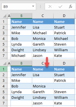
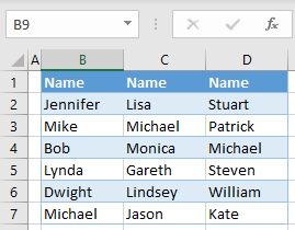
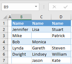
In Excel, you can easily delete all instances of a certain word using Replace functionality. Say you have the data set pictured below with names in Columns B, C, and D.
To delete all occurrences of Michael in the sheet (B7, C3, and D4), follow these steps:
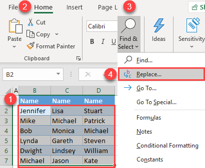
- Select the data range where you want to find and delete a word (B2:D7) and in the Ribbon, go to Home > Find & Select > Replace.
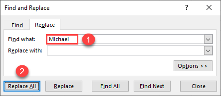
- In the Find and Replace window, enter the text you want to replace (Michael) for Find what, and click Replace All.
Leave the Replace with field empty to replace Michael with a blank. If you don’t know the full text string you want to delete, or you want to replace all cells containing just part of the text, you can use wildcard characters.
Every cell that had the word Michael before these changes is now blank.
Note: You can also use VBA code to achieve the same thing.
Find and Delete Words in Google Sheets
- Select the data range where you want to find and delete text (B2:D7) and in the Menu, go to Edit > Find and replace (or use the keyboard shortcut CTRL + H).
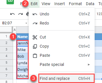
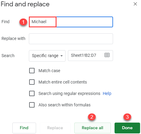
- In the pop-up window, enter the word you want to delete in the Find box and click Replace all, then Done.
The Replace with box is empty because you want to delete the word.
As a result, all cells that contained Michael are now empty.
Источник
Excel FIND and SEARCH functions with formula examples
 by Svetlana Cheusheva, updated on February 7, 2023
The tutorial explains the syntax of the Excel FIND and SEARCH functions and provides formula examples of advanced non-trivial uses.
In the last article, we covered the basics of the Excel Find and Replace dialog. In many situations, however, you may want Excel to find and extract data from other cells automatically based on your criteria. So, let’s have a closer look at what the Excel search functions have to offer.
Excel FIND function
The FIND function in Excel is used to return the position of a specific character or substring within a text string.
The syntax of the Excel Find function is as follows:
The first 2 arguments are required, the last one is optional.
- Find_text — the character or substring you want to find.
- Within_text — the text string to be searched within. Usually it’s supplied as a cell reference, but you can also type the string directly in the formula.
- Start_num — an optional argument that specifies from which character the search shall begin. If omitted, the search starts from the 1 st character of the within_text string.
If the FIND function does not find the find_text character(s), a #VALUE! error is returned.
For example, the formula =FIND(«d», «find») returns 4 because «d» is the 4 th letter in the word «find«. The formula =FIND(«a», «find») returns an error because there is no «a» in «find«. 
Excel FIND function — things to remember!
To correctly use a FIND formula in Excel, keep in mind the following simple facts:
- The FIND function is case sensitive. If you are looking for a case-insensitive match, use the SEARCH function.
- The FIND function in Excel does not allow using wildcard characters.
- If the find_text argument contains several characters, the FIND function returns the position of the first character. For example, the formula FIND(«ap»,»happy») returns 2 because «a» in the 2 nd letter in the word «happy».
- If within_text contains several occurrences of find_text, the first occurrence is returned. For example, FIND(«l», «hello») returns 3, which is the position of the first «l» character in the word «hello».
- If find_text is an empty string «», the Excel FIND formula returns the first character in the search string.
- The Excel FIND function returns the #VALUE! error if any of the following occurs:
- Find_text does not exist in within_text.
- Start_num contains more characters than within_text.
- Start_num is 0 (zero) or a negative number.
Excel SEARCH function
The SEARCH function in Excel is very similar to FIND in that it also returns the location of a substring in a text string. Is syntax and arguments are akin to those of FIND:
Unlike FIND, the SEARCH function is case-insensitive and it allows using the wildcard characters, as demonstrated in the following example.
And here’s a couple of basic Excel SEARCH formulas:
=SEARCH(«market», «supermarket») returns 6 because the substring «market» begins at the 6 th character of the word «supermarket».
=SEARCH(«e», «Excel») returns 1 because «e» is the first character in the word «Excel», ignoring the case.
Like FIND, Excel’s SEARCH function returns the #VALUE! error if:
- The value of the find_text argument is not found.
- The start_num argument is greater than the length of within_text.
- Start_num is equal to or less than zero.

Further on in this tutorial, you will find a few more meaningful formula examples that demonstrate how to use SEARCH function in Excel worksheets.
Excel FIND vs. Excel SEARCH
As already mentioned, the FIND and SEARCH functions in Excel are very much alike in terms of syntax and uses. However, they do have a couple of differences.
1. Case-sensitive FIND vs. case-insensitive SEARCH
The most essential difference between the Excel SEARCH and FIND functions is that SEARCH is case-insensitive, while FIND is case-sensitive.
For example, SEARCH(«e», «Excel») returns 1 because it ignores the case of «E», while FIND(«e», «Excel») returns 4 because it minds the case. 
2. Search with wildcard characters
Unlike FIND, the Excel SEARCH function accepts wildcard characters in the find_text argument:
- A question mark (?) matches one character, and
- An asterisk (*) matches any series of characters.
To see how it works on real data, consider the following example: 
As you see in the screenshot above, the formula SEARCH(«function*2013», A2) returns the position of the first character («f») in the substring if the text string referred to in the within_text argument contains both «function» and «2013», no matter how many other characters there are in between.
Tip. To find an actual question mark (?) or asterisk (*), type a tilde (
) before the corresponding character.
Excel FIND and SEARCH formula examples
In practice, the Excel FIND and SEARCH functions are rarely used on their own. Typically, you would utilize them in combination with other functions such as MID, LEFT or RIGHT, and the following formula examples demonstrate some real-life uses.
Example 1. Find a string preceding or following a given character
This example shows how you can find and extract all characters in a text string to the left or to the right of a specific character. To make things easier to understand, consider the following example.
Supposing you have a column of names (column A) and you want to pull the First name and Last name into separate columns.
To get the first name, you can use FIND (or SEARCH) in conjunction with the LEFT function:
=LEFT(A2, FIND(» «, A2)-1)
=LEFT(A2, SEARCH(» «, A2)-1)
As you probably know, the Excel LEFT function returns the specified number of left-most characters in a string. And you use the FIND function to determine the position of a space (» «) to let the LEFT function know how many characters to extract. At that, you subtract 1 from the space’s position because you don’t want the returned value to include the space.
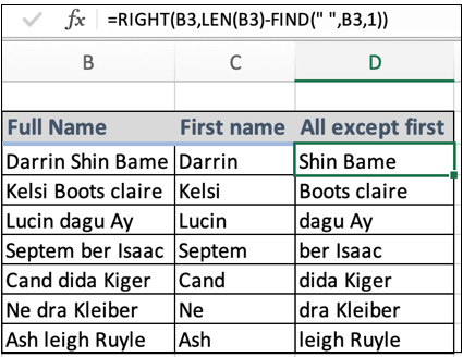
To extract the last name, use the combination of the RIGHT, FIND / SEARCH and LEN functions. The LEN function is needed to get the total number of characters in the string, from which you subtract the position of the space:
The following screenshot demonstrates the result: 
For more complex scenarios, such as extracting a middle name or splitting names with suffixes, please see How to split cells in Excel using formulas.
Example 2. Find Nth occurrence of a given character in a text string
Supposing you have some text strings in column A, say a list of SKUs, and you want to find the position of the 2 nd dash in a string. The following formula works a treat:
The first two arguments are easy to interpret: locate a dash («-«) in cell A2. In the third argument (start_num), you embed another FIND function that tells Excel to start searching beginning with the character that comes right after the first occurrence of dash (FIND(«-«,A2)+1).
To return the position of the 3 rd occurrence, you embed the above formula in the start_num argument of another FIND function and add 2 to the returned value:
=FIND(«-«,A2, FIND(«-«, A2, FIND(«-«,A2)+1) +2) 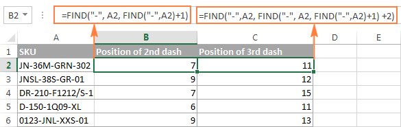
Another and probably a simpler way of finding the Nth occurrence of a given character is using the Excel FIND function in combination with CHAR and SUBSTITUTE:
Where «-» is the character in question and «3» is the Nth occurrence you want to find.
In the above formula, the SUBSTITUTE function replaces the 3rd occurrence of dash («-«) with CHAR(1), which is the unprintable «Start of Heading» character in the ASCII system. Instead of CHAR(1) you can use any other unprintable character from 1 to 31. And then, the FIND function returns the position of that character in the text string. So, the general formula is as follows:
At first sight, it may seem that the above formulas have little practical value, but the next example will show how useful they are in solving real tasks.
Note. Please remember that the Excel FIND function is case-sensitive. In our example, this makes no difference, but if you are working with letters and you want a case-insensitive match, use the SEARCH function instead of FIND.
To locate a substring of a given length within any text string, use Excel FIND or Excel SEARCH in combination with the MID function. The following example demonstrates how you can use such formulas in practice.
In our list of SKUs, supposing you want to find the first 3 characters following the first dash and pull them in another column.
If the group of characters preceding the first dash always contains the same number of items (e.g. 2 chars) this would be a trivial task. You could use the MID function to return 3 characters from a string, starting at position 4 (skipping the first 2 characters and a dash):
Translated into English, the formula says: «Look in cell A2, begin extracting from character 4, and return 3 characters». 
However, in real-life worksheets, the substring you need to extract could start anywhere within the text string. In our example, you may not know how many characters precede the first dash. To cope with this challenge, use the FIND function to determine the starting point of the substring that you want to retrieve.
The FIND formula to return the position of the 1 st dash is as follows:
Because you want to start with the character that follows the dash, add 1 to the returned value and embed the above function in the second argument (start_num) of the MID function:
In this scenario, the Excel SEARCH function works equally well:
=MID(A2, SEARCH(«-«,A2)+1, 3) 
It’s great, but what if the group of chars following the first dash contains a different number of characters? Hmm. this might be a problem: 
As you see in the above screenshot, the formula works perfectly for rows 1 and 2. In rows 4 and 5, the second group contains 4 characters, but only the first 3 chars are returned. In rows 6 and 7, there are only 2 characters in the second group, and therefore our Excel Search formula returns a dash following them.
If you wanted to return all chars between the 1 st and 2 nd occurrences of a certain character (dash in this example), how would you proceed? Here is the answer:
=MID(A2, FIND(«-«,A2)+1, FIND(«-«, A2, FIND(«-«,A2)+1) — FIND(«-«,A2)-1) 
For better understanding of this MID formula, let’s examine its arguments one by one:
- 1 st argument (text). It’s the text string containing the characters you want to extract, cell A2 in this example.
- 2 nd argument (start_position). Specifies the position of the first character you want to extract. You use the FIND function to locate the first dash in the string and add 1 to that value because you want to start with the character that follows the dash: FIND(«-«,A2)+1.
- 3 rd argument (num_chars). Specifies the number of characters you want to return. In our formula, this is the trickiest part. You use two FIND (or SEARCH) functions, one determines the position of the first dash: FIND(«-«,A2). And the other returns the position of the second dash: FIND(«-«, A2, FIND(«-«,A2)+1). Then you subtract the former from the latter, and then subtract 1 because you don’t want to include either dash. As the result, you will get the number of characters between the 1 st and 2 nd dashes, which is exactly what we are looking for. So, you feed that value to the num_chars argument of the MID function.
In a similar fashion, you can return 3 characters after the 2 nd dash:
=MID(A2, FIND(«-«,A2, FIND(«-«, A2, FIND(«-«,A2)+1) +2), 3)
Or, extract all the characters between the 2 nd and 3 rd dashes:
=MID(A2, FIND(«-«, A2, FIND(«-«,A2)+1)+1, FIND(«-«,A2, FIND(«-«, A2, FIND(«-«,A2)+1) +2) — FIND(«-«, A2, FIND(«-«,A2)+1)-1) 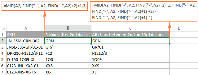
Example 4. Find text between parentheses
Supposing you have some long text string in column A and you want to find and extract only the text enclosed in (parentheses).
To do this, you would need the MID function to return the desired number of characters from a string, and either Excel FIND or SEARCH function to determine where to start and how many characters to extract.
The logic of this formula is similar to the ones we discussed in the previous example. And again, the most complex part is the last argument that tells the formula how many characters to return. That pretty long expression in the num_chars argument does the following:
- First, you find the position of the closing parenthesis: SEARCH(«)»,A2)
- After that you locate the position of the opening parenthesis: SEARCH(«(«,A2)
- And then, you calculate the difference between the positions of the closing and opening parentheses and subtract 1 from that number, because you don’t want either parenthesis in the result: SEARCH(«)»,A2)-SEARCH(«(«,A2))-1

Naturally, nothing prevents you from using the Excel FIND function instead of SEARCH, because case-sensitivity or case-insensitivity makes no difference in this example.
Hopefully, this tutorial has shed some light on how to use SEARCH and FIND functions in Excel. In the next tutorial, we are going to closely examine the REPLACE function, so please stay tuned. Thank you for reading!
Источник
SEARCH, SEARCHB functions
Excel for Microsoft 365 Excel for Microsoft 365 for Mac Excel for the web Excel 2021 Excel 2021 for Mac Excel 2019 Excel 2019 for Mac Excel 2016 Excel 2016 for Mac Excel 2013 Excel 2010 Excel 2007 Excel for Mac 2011 Excel Starter 2010 More…Less
This article describes the formula syntax and usage of the SEARCH and SEARCHB functions in Microsoft Excel.
Description
The SEARCH and SEARCHB functions locate one text string within a second text string, and return the number of the starting position of the first text string from the first character of the second text string. For example, to find the position of the letter «n» in the word «printer», you can use the following function:
=SEARCH(«n»,»printer»)
This function returns 4 because «n» is the fourth character in the word «printer.»
You can also search for words within other words. For example, the function
=SEARCH(«base»,»database»)
returns 5, because the word «base» begins at the fifth character of the word «database». You can use the SEARCH and SEARCHB functions to determine the location of a character or text string within another text string, and then use the MID and MIDB functions to return the text, or use the REPLACE and REPLACEB functions to change the text. These functions are demonstrated in Example 1 in this article.
Important:
-
These functions may not be available in all languages.
-
SEARCHB counts 2 bytes per character only when a DBCS language is set as the default language. Otherwise SEARCHB behaves the same as SEARCH, counting 1 byte per character.
The languages that support DBCS include Japanese, Chinese (Simplified), Chinese (Traditional), and Korean.
Syntax
SEARCH(find_text,within_text,[start_num])
SEARCHB(find_text,within_text,[start_num])
The SEARCH and SEARCHB functions have the following arguments:
-
find_text Required. The text that you want to find.
-
within_text Required. The text in which you want to search for the value of the find_text argument.
-
start_num Optional. The character number in the within_text argument at which you want to start searching.
Remark
-
The SEARCH and SEARCHB functions are not case sensitive. If you want to do a case sensitive search, you can use FIND and FINDB.
-
You can use the wildcard characters — the question mark (?) and asterisk (*) — in the find_text argument. A question mark matches any single character; an asterisk matches any sequence of characters. If you want to find an actual question mark or asterisk, type a tilde (~) before the character.
-
If the value of find_text is not found, the #VALUE! error value is returned.
-
If the start_num argument is omitted, it is assumed to be 1.
-
If start_num is not greater than 0 (zero) or is greater than the length of the within_text argument, the #VALUE! error value is returned.
-
Use start_num to skip a specified number of characters. Using the SEARCH function as an example, suppose you are working with the text string «AYF0093.YoungMensApparel». To find the position of the first «Y» in the descriptive part of the text string, set start_num equal to 8 so that the serial number portion of the text (in this case, «AYF0093») is not searched. The SEARCH function starts the search operation at the eighth character position, finds the character that is specified in the find_text argument at the next position, and returns the number 9. The SEARCH function always returns the number of characters from the start of the within_text argument, counting the characters you skip if the start_num argument is greater than 1.
Examples
Copy the example data in the following table, and paste it in cell A1 of a new Excel worksheet. For formulas to show results, select them, press F2, and then press Enter. If you need to, you can adjust the column widths to see all the data.
|
Data |
||
|---|---|---|
|
Statements |
||
|
Profit Margin |
||
|
margin |
||
|
The «boss» is here. |
||
|
Formula |
Description |
Result |
|
=SEARCH(«e»,A2,6) |
Position of the first «e» in the string in cell A2, starting at the sixth position. |
7 |
|
=SEARCH(A4,A3) |
Position of «margin» (string for which to search is cell A4) in «Profit Margin» (cell in which to search is A3). |
8 |
|
=REPLACE(A3,SEARCH(A4,A3),6,»Amount») |
Replaces «Margin» with «Amount» by first searching for the position of «Margin» in cell A3, and then replacing that character and the next five characters with the string «Amount.» |
Profit Amount |
|
=MID(A3,SEARCH(» «,A3)+1,4) |
Returns the first four characters that follow the first space character in «Profit Margin» (cell A3). |
Marg |
|
=SEARCH(«»»»,A5) |
Position of the first double quotation mark («) in cell A5. |
5 |
|
=MID(A5,SEARCH(«»»»,A5)+1,SEARCH(«»»»,A5,SEARCH(«»»»,A5)+1)-SEARCH(«»»»,A5)-1) |
Returns only the text enclosed in the double quotation marks in cell A5. |
boss |
Need more help?
![]()
Download Article
![]()
Download Article
An Excel document can be overwhelming to look through. Thankfully, you can use the search function to conveniently locate a particular word, or group of words, in an Excel worksheet.
-

1
Launch MS Excel. Do this by clicking on its icon in your desktop. It is the green X icon with spreadsheets in its background.
- If you don’t have an Excel shortcut icon on your desktop, find it in your Start menu and click the icon there.
-
2
Find the Excel file you want to open. Click “File” in the upper left corner of the window then click “Open.” A file browser will appear. Browse your computer for the Excel file you want to open.
Advertisement
-
3
Open the file. Once you’ve located the file, click on it to select then click “Open” in the lower-right portion of the file browser.


Advertisement
-
1
Click a cell. Once you’re in the worksheet, click on any cell on the worksheet to ensure that the window is active.
-
2
Open the Find/Replace With window. Hit the key combination Ctrl + F on your keyboard. A new window will appear with two fields: “Find” and “Replace with.”
-
3
Type in the words you want to find. Enter the exact word or phrase you want to search for, and click on the “Find” button in the lower right of the Find window.
- Excel will begin searching for matches of the word, or words, you entered in the search field. All words in the document that matches those you entered will be highlighted to help you better locate them.


Advertisement
Ask a Question
200 characters left
Include your email address to get a message when this question is answered.
Submit
Advertisement
Thanks for submitting a tip for review!
About This Article
Thanks to all authors for creating a page that has been read 91,003 times.
Is this article up to date?
In this article, we will learn How to Extract all the words except the first in Excel.
Scenario :
Working with text data in excel. Sometimes we come across the problem of splitting words from the full text. For example splitting full names into first name and last name. Or extracting the names from the given email ids. For situations like these we use LEFT and RIGHT functions in excel along with some basic sense of how excel functions work. How to recognize where to separate the full name like Nedra Kleiber. Here a space character in between the first name and last name. So we direct excel to find the position of first space char in the full name and separate it into two using functions
First name and rest name formula in Excel
Here given a name value as text in the formula. First of all the find function gives the position of first space character and LEN function gives the length of full text. Now the RIGHT function has everything to extract the word.
Remaining name formula syntax:
=RIGHT (text, LEN (text) — FIND (» «, text, 1 ) )
text : full name
» » : Space character given in quotes. Or use char function
1 : nth occurrence of space char. (here 1 is used to specify first occurrence)
First name formula syntax:
text : full name
» » : Space character given in quotes. Or use char function
1 : nth occurrence of space char. (here 1 is used to specify first occurrence)
Example :
All of these might be confusing to understand. Let’s understand how to use the function using an example. Here we are given some sample names and we need to extract the first name and rest of the name in another column. So first we start with a basic formula that is first name extraction. You can provide text values using text in quotes or by using cell reference which is explained here.
First name formula:
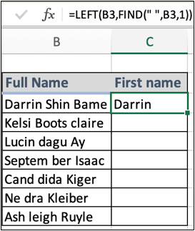
Copy and paste the formula in other cells either using CTRL + D or just by stretching the right bottom box of the C3 cell.

As you can see in the above snapshot all the first names are here. Now either you can substitute the first name from the full name with blank to get the last name or use the last name formula explained below.
To get the Last name directly from the full name using the RIGHT function formula is shown below.
Remaining or last name formula:
Copy and paste the formula to different required cells using Ctrl + D or dragging down the right bottom corner of the D3 cell.

As you can see the first name and last name both in different columns separated using the simple excel formulas. Learn more about excel formulas here.
Here are all the observational notes using the formula in Excel
Notes :
- Text values in formula be used with between quotes or using cell reference. Using cell reference in excel is the best common practice.
- Use the =CHAR(32) function to get the space character in the formula.
Hope this article about How to Extract all the words except the first in Excel is explanatory. Find more articles on calculating values and related Excel formulas here. If you liked our blogs, share it with your friends on Facebook. And also you can follow us on Twitter and Facebook. We would love to hear from you, do let us know how we can improve, complement or innovate our work and make it better for you. Write to us at info@exceltip.com.
Related Articles :
Data Validation in Excel : Data Validation is a tool used to restrict users to input value manually in cell or worksheet in Excel. It has a list of options to choose from.
Way to use Vlookup function in Data Validation : Restrict users to allow values from the lookup table using Data validation formula box in Excel. Formula box in data validation allows you to choose the type of restriction required.
Restrict Dates using Data Validation : Restrict user to allow dates from a given range in cell which lays within Excel date format in Excel.
How to give the error messages in Data Validation : Restrict users to customize input information in the worksheet and guide the input information through error messages under data validation in Excel.
Create Drop Down Lists in Excel using Data Validation : Restrict users to allow values from the drop down list using Data validation List option in Excel. List box in data validation allows you to choose the type of restriction required.
Popular Articles :
50 Excel Shortcuts to Increase Your Productivity : Get faster at your tasks in Excel. These shortcuts will help you increase your work efficiency in Excel.
How to use the VLOOKUP Function in Excel : This is one of the most used and popular functions of excel that is used to lookup value from different ranges and sheets.
How to use the IF Function in Excel : The IF statement in Excel checks the condition and returns a specific value if the condition is TRUE or returns another specific value if FALSE.
How to use the SUMIF Function in Excel : This is another dashboard essential function. This helps you sum up values on specific conditions.
How to use the COUNTIF Function in Excel : Count values with conditions using this amazing function. You don’t need to filter your data to count specific values. Countif function is essential to prepare your dashboard.
Write this function in a module:
Public Function WordFinder(searchRange As Range, seekWord As String, iteration As Integer)
    Dim rangeCell As Range      'holder cell used in For-Each loop
    Dim rangeText As String     'holder for rangeCell's text
    Dim counter As Integer

    counter = 0
    'loop through cells in the range
    For Each rangeCell In searchRange.Cells
        rangeText = rangeCell.Value 'capture the current cell value
        'check if the seek word appears in the current cell
        If InStr(rangeText, seekWord) > 0 Then
            counter = counter + 1 'increment the occurrence counter
            If counter = iteration Then 'this is the occurrence we're looking for
                'return it
                WordFinder = rangeText
                Exit Function
            End If
        End If
    Next rangeCell
    WordFinder = "n/a" 'that occurrence number was not found

End Function
And across the top row of your results sheet, enter this formula in each cell:
=wordfinder(Sheet2!$A1:$A8,"apple",column())
column() increments with each column, so as you copy/paste it across the top row, it’s counting up. The dollar signs make sure the reference remains absolutely on column A.
The 2nd parameter («apple») can come from a cell, although I’ve hard-coded it here.
There might be a more elegant way to do this, but this is a quick & dirty way that should work.