Find all tables excel - Word и Excel - помощь в работе с программами

Содержание

Use Excel built-in functions to find data in a table or a range of cells
Summary
Create the Sample Worksheet
Term Definitions
Functions
LOOKUP()
VLOOKUP()
INDEX() and MATCH()
OFFSET() and MATCH()
Finding Data Tables in Excel
3 Answers 3
Look up values with VLOOKUP, INDEX, or MATCH
Using INDEX and MATCH instead of VLOOKUP
Give it a try
VLOOKUP Example at work
Locating all the tables on one spreadsheet using Excel VBA
Trying to find all the data tables in my workbook
jamie_in_nj
Excel Facts
Jerry Sullivan
jamie_in_nj
Jerry Sullivan
jamie_in_nj
Jerry Sullivan

Use Excel built-in functions to find data in a table or a range of cells

Summary

This step-by-step article describes how to find data in a table (or range of cells) by using various built-in functions in Microsoft Excel. You can use different formulas to get the same result.

Create the Sample Worksheet

This article uses a sample worksheet to illustrate Excel built-in functions. Consider the example of referencing a name from column A and returning the age of that person from column C. To create this worksheet, enter the following data into a blank Excel worksheet.

You will type the value that you want to find into cell E2. You can type the formula in any blank cell in the same worksheet.

Term Definitions

This article uses the following terms to describe the Excel built-in functions:

The whole lookup table

The value to be found in the first column of Table_Array.

Lookup_Array
-or-
Lookup_Vector

The range of cells that contains possible lookup values.

The column number in Table_Array the matching value should be returned for.

3 (third column in Table_Array)

Result_Array
-or-
Result_Vector

A range that contains only one row or column. It must be the same size as Lookup_Array or Lookup_Vector.

A logical value (TRUE or FALSE). If TRUE or omitted, an approximate match is returned. If FALSE, it will look for an exact match.

This is the reference from which you want to base the offset. Top_Cell must refer to a cell or range of adjacent cells. Otherwise, OFFSET returns the #VALUE! error value.

This is the number of columns, to the left or right, that you want the upper-left cell of the result to refer to. For example, «5» as the Offset_Col argument specifies that the upper-left cell in the reference is five columns to the right of reference. Offset_Col can be positive (which means to the right of the starting reference) or negative (which means to the left of the starting reference).

Functions

LOOKUP()

The LOOKUP function finds a value in a single row or column and matches it with a value in the same position in a different row or column.

The following is an example of LOOKUP formula syntax:

The following formula finds Mary’s age in the sample worksheet:

The formula uses the value «Mary» in cell E2 and finds «Mary» in the lookup vector (column A). The formula then matches the value in the same row in the result vector (column C). Because «Mary» is in row 4, LOOKUP returns the value from row 4 in column C (22).

NOTE: The LOOKUP function requires that the table be sorted.

For more information about the LOOKUP function, click the following article number to view the article in the Microsoft Knowledge Base:

VLOOKUP()

The VLOOKUP or Vertical Lookup function is used when data is listed in columns. This function searches for a value in the left-most column and matches it with data in a specified column in the same row. You can use VLOOKUP to find data in a sorted or unsorted table. The following example uses a table with unsorted data.

The following is an example of VLOOKUP formula syntax:

The following formula finds Mary’s age in the sample worksheet:

The formula uses the value «Mary» in cell E2 and finds «Mary» in the left-most column (column A). The formula then matches the value in the same row in Column_Index. This example uses «3» as the Column_Index (column C). Because «Mary» is in row 4, VLOOKUP returns the value from row 4 in column C (22).

For more information about the VLOOKUP function, click the following article number to view the article in the Microsoft Knowledge Base:

INDEX() and MATCH()

You can use the INDEX and MATCH functions together to get the same results as using LOOKUP or VLOOKUP.

The following is an example of the syntax that combines INDEX and MATCH to produce the same results as LOOKUP and VLOOKUP in the previous examples:

The following formula finds Mary’s age in the sample worksheet:

The formula uses the value «Mary» in cell E2 and finds «Mary» in column A. It then matches the value in the same row in column C. Because «Mary» is in row 4, the formula returns the value from row 4 in column C (22).

NOTE: If none of the cells in Lookup_Array match Lookup_Value («Mary»), this formula will return #N/A.
For more information about the INDEX function, click the following article number to view the article in the Microsoft Knowledge Base:

OFFSET() and MATCH()

You can use the OFFSET and MATCH functions together to produce the same results as the functions in the previous example.

The following is an example of syntax that combines OFFSET and MATCH to produce the same results as LOOKUP and VLOOKUP:

This formula finds Mary’s age in the sample worksheet:

The formula uses the value «Mary» in cell E2 and finds «Mary» in column A. The formula then matches the value in the same row but two columns to the right (column C). Because «Mary» is in column A, the formula returns the value in row 4 in column C (22).

For more information about the OFFSET function, click the following article number to view the article in the Microsoft Knowledge Base:

Источник

Finding Data Tables in Excel

I have inherited a spreadsheet which contains several data tables. I know this because when I recalculate the spreadsheet takes time to recalculate the tables, and shows this in the recalculation notifier. Is there a systematic way to locate these data tables, similarly to locating links ( the spreadsheet has > 50 worksheets, so just searching sheet by sheet would be a little tedious).

3 Answers 3

You haven’t said / tagged what version of Excel you are using, but since you call them Tables, not Lists, I assume it is 2007 or 2010. If you go to Formulas tab of the Ribbon > Name Manager you will see Table names listed amongst other defined names. They show a different icon next to them, but to make things even clearer you can use the Filter button at the top right to show tables only.

As you work out what they do it is with renaming tables to sensible names (from the Table Tools > Design ribbon or the Name Manager) and possibly adding comments about their purpose to remind you later (do this in Name Manager > Edit)

In later versions of Excel you can:

This will bring up a list of named items, including tables, that you can then navigate directly to

If the Name Manager shows no tables and a ctrl+F search for «=table» yields no results, but you are still calculating data tables, check for hidden tabs in your workbook that may include data tables.

Источник

Look up values with VLOOKUP, INDEX, or MATCH

Tip: Try using the new XLOOKUP and XMATCH functions, improved versions of the functions described in this article. These new functions work in any direction and return exact matches by default, making them easier and more convenient to use than their predecessors.

Suppose that you have a list of office location numbers, and you need to know which employees are in each office. The spreadsheet is huge, so you might think it is challenging task. It’s actually quite easy to do with a lookup function.

The VLOOKUP and HLOOKUP functions, together with INDEX and MATCH, are some of the most useful functions in Excel.

Note: The Lookup Wizard feature is no longer available in Excel.

Here’s an example of how to use VLOOKUP.

In this example, B2 is the first argument—an element of data that the function needs to work. For VLOOKUP, this first argument is the value that you want to find. This argument can be a cell reference, or a fixed value such as «smith» or 21,000. The second argument is the range of cells, C2-:E7, in which to search for the value you want to find. The third argument is the column in that range of cells that contains the value that you seek.

The fourth argument is optional. Enter either TRUE or FALSE. If you enter TRUE, or leave the argument blank, the function returns an approximate match of the value you specify in the first argument. If you enter FALSE, the function will match the value provide by the first argument. In other words, leaving the fourth argument blank—or entering TRUE—gives you more flexibility.

This example shows you how the function works. When you enter a value in cell B2 (the first argument), VLOOKUP searches the cells in the range C2:E7 (2nd argument) and returns the closest approximate match from the third column in the range, column E (3rd argument).

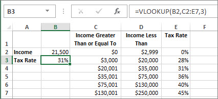
The fourth argument is empty, so the function returns an approximate match. If it didn’t, you’d have to enter one of the values in columns C or D to get a result at all.

When you’re comfortable with VLOOKUP, the HLOOKUP function is equally easy to use. You enter the same arguments, but it searches in rows instead of columns.

Using INDEX and MATCH instead of VLOOKUP

There are certain limitations with using VLOOKUP—the VLOOKUP function can only look up a value from left to right. This means that the column containing the value you look up should always be located to the left of the column containing the return value. Now if your spreadsheet isn’t built this way, then do not use VLOOKUP. Use the combination of INDEX and MATCH functions instead.

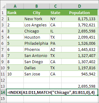
This example shows a small list where the value we want to search on, Chicago, isn’t in the leftmost column. So, we can’t use VLOOKUP. Instead, we’ll use the MATCH function to find Chicago in the range B1:B11. It’s found in row 4. Then, INDEX uses that value as the lookup argument, and finds the population for Chicago in the 4th column (column D). The formula used is shown in cell A14.

For more examples of using INDEX and MATCH instead of VLOOKUP, see the article https://www.mrexcel.com/excel-tips/excel-vlookup-index-match/ by Bill Jelen, Microsoft MVP.

Give it a try

If you want to experiment with lookup functions before you try them out with your own data, here’s some sample data.

VLOOKUP Example at work

Copy the following data into a blank spreadsheet.

Tip: Before you paste the data into Excel, set the column widths for columns A through C to 250 pixels, and click Wrap Text ( Home tab, Alignment group).

Источник

Locating all the tables on one spreadsheet using Excel VBA

I have a few spreadsheets with various tables in different formats. My task is to locate and identify anything on the spreadsheets that can be considered a table, and flatten it into a text file. Currently I am only looking for a solution to locate all tables on one spreadsheet.

Spreadsheet format is somewhat fixed, I have to process what I am given.
A completely empty line can split a table into two, unless there’s a sure way to tell what is a missing line within one table and what is an actual new table.
I can handle merged fields beforehand if needs be (split them and backfill with the common value, that’s already written and is working)
The tables could have a different number of columns, different header rows, and they could begin in any column.
I consider records in the same line to be part of the same table, I am not expecting to find tables next to one another.

The code I have so far as follows:

The sample sheet I am looking at is as messy as possible to account for «creative» formatting.

The error I’m getting is due to the fact that the second table starts from B7 and ends in E1048576, which is well past the loop condition — I would like this range to end in E8 (or E9 if possible or once the merged cells are broken up).

Источник

Trying to find all the data tables in my workbook

jamie_in_nj

Board Regular

Excel Facts

Jerry Sullivan

MrExcel MVP

I don’t know why the Name Manager is going blank when you filter for Tables.

You could try using this code to list the names and adddresses of each Table in your Workbook.

jamie_in_nj

Board Regular

Jerry Sullivan

MrExcel MVP

Hmm..perhaps those aren’t ListObjects but some other type of Table-like Object.

This forum doesn’t support attachments- when necessary people either post to a sharing site like Box.com or exchange email addresses through a Private Message (PM).

If you post it, or send me a PM, I’ll take a look.

jamie_in_nj

Board Regular

Jerry Sullivan

MrExcel MVP

I reviewed your file and can see why the tables don’t show up in the Name Manager and my code didn’t count the tables.

I had assumed that these were ListObject tables, which can be created by:
Selecting a valid range then from the Ribbon > Insert > Table

These ListObjects were called Lists prior to xl2007, and they are now commonly referred to as «Tables».
ListObjects show up in the Name Manager and you can filter the Names to just show «Tables».

What you have in your file are not «ListObjects» but rather «Data Tables» (Which is exactly what you’ve correctly called them from the beginning, so the misunderstanding is mine!)

I haven’t had experience with Data Tables, so I appreciate that you’ve helped me become aware of them.

In Excel 2010 Tables can be created from the Ribbon through Data > What-If-Analysis > Data Table.
This link provides some instructions
Calculate multiple results by using a data table — Excel — Office.com

So now that we understand why the Name Manager and ListObject Macro didn’t work, we can revisit the problem you are trying to solve.

Here’s my uncertain understanding and I welcome corrections from others who have more knowledge on this:

Data Tables are not Objects within the Excel Object Model, so they can’t be easily counted or listed the same way ListObjects, PivotTables or Shape Objects can be handled with VBA. Rather they are Array formulas that use the TABLE() function leaving a formula that looks like <=TABLE(,B7)>where B7 is the «What If» Column Input.

One approach to counting/listing the Data Tables could be to use VBA to search all formulas and gather unique instances of «TABLE(*,*)». That seems more complicated than it should be, so I’ll wait a bit to see if someone else can share a better approach.

Источник

asked Jul 5, 2011 at 21:34

You haven’t said / tagged what version of Excel you are using, but since you call them Tables, not Lists, I assume it is 2007 or 2010.
If you go to Formulas tab of the Ribbon > Name Manager you will see Table names listed amongst other defined names.
They show a different icon next to them, but to make things even clearer you can use the Filter button at the top right to show tables only.

answered Jul 6, 2011 at 15:32

AdamVAdamV

6,0281 gold badge22 silver badges38 bronze badges

In later versions of Excel you can:

Home -> Find & Select -> Go To

This will bring up a list of named items, including tables, that you can then navigate directly to

answered Jun 16, 2016 at 1:01

That was the source of my problem.

answered Oct 30, 2015 at 22:01

Источник

Hi jamie_in_nj,

I don’t know why the Name Manager is going blank when you filter for Tables.

You could try using this code to list the names and adddresses of each Table in your Workbook.

Code:

Sub List_Tables_In_Workbook()
    Dim wsSummary As Worksheet
    Dim tbl As ListObject
    Dim n As Long, lRow As Long

    
    '--add summary sheet with headers
    Set wsSummary = Worksheets.Add(Before:=Sheets(1))
    Range("A1:C1") = Array("Table Name", _
        "Found on Sheet", "at Range Address")
    lRow = 1 'Header Row

    
    '--step through each sheet and list each table
    For n = 2 To Worksheets.Count
        For Each tbl In Worksheets(n).ListObjects
            lRow = lRow + 1
            With wsSummary
                .Cells(lRow, "A") = tbl.Name
                .Cells(lRow, "B") = tbl.Parent.Name
                .Cells(lRow, "C") = tbl.Range.Address
            End With
        Next tbl
    Next n

    
End Sub

Hi thanks for the response. The code does not seem to list my data tables though. I tried it in the one workbook I had. It created a new worksheet. That sheet just has the headers of Table Name, Found on Sheet, and at Range Address, but nothing below them. I created simple workbook and created a Data Table, and tried it again, and got the same result. I can post the simple workbook here, if people do that. Sorry, I am not familiar with the protocol on the site, and if I should post a workbook. Thanks for any help!

Hmm..perhaps those aren’t ListObjects but some other type of Table-like Object.

This forum doesn’t support attachments- when necessary people either post to a sharing site like Box.com or exchange email addresses through a Private Message (PM).

If you post it, or send me a PM, I’ll take a look.

Thanks I sent you a PM. If you are OK with PM-ing me back with your email address, I will send you a simple example workbook.

Hi Jamie,

I reviewed your file and can see why the tables don’t show up in the Name Manager and my code didn’t count the tables.

I had assumed that these were ListObject tables, which can be created by:
Selecting a valid range then from the Ribbon > Insert > Table

These ListObjects were called Lists prior to xl2007, and they are now commonly referred to as «Tables».
ListObjects show up in the Name Manager and you can filter the Names to just show «Tables».

What you have in your file are not «ListObjects» but rather «Data Tables» (Which is exactly what you’ve correctly called them from the beginning, so the misunderstanding is mine!)

I haven’t had experience with Data Tables, so I appreciate that you’ve helped me become aware of them.

In Excel 2010 Tables can be created from the Ribbon through Data > What-If-Analysis > Data Table…
This link provides some instructions

Calculate multiple results by using a data table — Excel — Office.com

So now that we understand why the Name Manager and ListObject Macro didn’t work, we can revisit the problem you are trying to solve.

Here’s my uncertain understanding and I welcome corrections from others who have more knowledge on this:

Data Tables are not Objects within the Excel Object Model, so they can’t be easily counted or listed the same way ListObjects, PivotTables or Shape Objects can be handled with VBA. Rather they are Array formulas that use the TABLE() function leaving a formula that looks like {=TABLE(,B7)} where B7 is the «What If» Column Input.

Last edited: Aug 9, 2013

Hi Jamie,
One approach to counting/listing the Data Tables could be to use VBA to search all formulas and gather unique instances of «TABLE(*,*)». That seems more complicated than it should be, so I’ll wait a bit to see if someone else can share a better approach.

I’d be inclined to go this route Jerry as I can’t think of any other distinctive feature of a Data Table. These can take a long time to calculate and with 21 of them it must be nearly a lifetime so it’s worth finding and eliminating them where possible. When I use them, I always set Formulas>Calculations to «Automatic Except for Data Tables» which avoids long waits when anything triggers a calculation.

Hi Jerry, thanks for doing the research, and suggestion, and thanks to Joe as well.

Currently the calculation happens fairly quickly, within seconds, so I am OK with the timing. I am able to find the Data Tables by going through and visually looking for them. The functionality is quite helpful, although their setup was not that intuitive to me, but I have gotten past that hurdle.

Jamie

I was searching for a solution for this and figured it out based on reading the thread so I thought I would leave my findings for future searchers… if you you use the Find feature (Ctrl-F) and search for «Table(» it will find all the cells that are part of a «Data Table» (What-if analysis result). Remember to change the ‘Within’ field in Advanced to «Workbook» if you want to find across multiple worksheets

Hi msweetmo,

Welcome to MrExcel and thank you for sharing your findings.

Источник

Summary

This step-by-step article describes how to find data in a table (or range of cells) by using various built-in functions in Microsoft Excel. You can use different formulas to get the same result.

Create the Sample Worksheet

You will type the value that you want to find into cell E2. You can type the formula in any blank cell in the same worksheet.

	A	B	C	D	E
1	Name	Dept	Age		Find Value
2	Henry	501	28		Mary
3	Stan	201	19
4	Mary	101	22
5	Larry	301	29

Term Definitions

This article uses the following terms to describe the Excel built-in functions:

Term	Definition	Example
Table Array	The whole lookup table	A2:C5
Lookup_Value	The value to be found in the first column of Table_Array.	E2
Lookup_Array -or- Lookup_Vector	The range of cells that contains possible lookup values.	A2:A5
Col_Index_Num	The column number in Table_Array the matching value should be returned for.	3 (third column in Table_Array)
Result_Array -or- Result_Vector	A range that contains only one row or column. It must be the same size as Lookup_Array or Lookup_Vector.	C2:C5
Range_Lookup	A logical value (TRUE or FALSE). If TRUE or omitted, an approximate match is returned. If FALSE, it will look for an exact match.	FALSE
Top_cell	This is the reference from which you want to base the offset. Top_Cell must refer to a cell or range of adjacent cells. Otherwise, OFFSET returns the #VALUE! error value.
Offset_Col	This is the number of columns, to the left or right, that you want the upper-left cell of the result to refer to. For example, «5» as the Offset_Col argument specifies that the upper-left cell in the reference is five columns to the right of reference. Offset_Col can be positive (which means to the right of the starting reference) or negative (which means to the left of the starting reference).

Functions

LOOKUP()

The LOOKUP function finds a value in a single row or column and matches it with a value in the same position in a different row or column.

The following is an example of LOOKUP formula syntax:

=LOOKUP(Lookup_Value,Lookup_Vector,Result_Vector)

The following formula finds Mary’s age in the sample worksheet:

=LOOKUP(E2,A2:A5,C2:C5)

NOTE: The LOOKUP function requires that the table be sorted.

For more information about the LOOKUP function, click the following article number to view the article in the Microsoft Knowledge Base:

How to use the LOOKUP function in Excel

VLOOKUP()

The VLOOKUP or Vertical Lookup function is used when data is listed in columns. This function searches for a value in the left-most column and matches it with data in a specified column in the same row. You can use VLOOKUP to find data in a sorted or unsorted table. The following example uses a table with unsorted data.

The following is an example of VLOOKUP formula syntax:

=VLOOKUP(Lookup_Value,Table_Array,Col_Index_Num,Range_Lookup)

The following formula finds Mary’s age in the sample worksheet:

=VLOOKUP(E2,A2:C5,3,FALSE)

The formula uses the value «Mary» in cell E2 and finds «Mary» in the left-most column (column A). The formula then matches the value in the same row in Column_Index. This example uses «3» as the Column_Index (column C). Because «Mary» is in row 4, VLOOKUP returns the value from row 4 in column C (22).

For more information about the VLOOKUP function, click the following article number to view the article in the Microsoft Knowledge Base:

How to Use VLOOKUP or HLOOKUP to find an exact match

INDEX() and MATCH()

You can use the INDEX and MATCH functions together to get the same results as using LOOKUP or VLOOKUP.

The following is an example of the syntax that combines INDEX and MATCH to produce the same results as LOOKUP and VLOOKUP in the previous examples:

=INDEX(Table_Array,MATCH(Lookup_Value,Lookup_Array,0),Col_Index_Num)

The following formula finds Mary’s age in the sample worksheet:

=INDEX(A2:C5,MATCH(E2,A2:A5,0),3)

NOTE: If none of the cells in Lookup_Array match Lookup_Value («Mary»), this formula will return #N/A.
For more information about the INDEX function, click the following article number to view the article in the Microsoft Knowledge Base:

How to use the INDEX function to find data in a table

OFFSET() and MATCH()

You can use the OFFSET and MATCH functions together to produce the same results as the functions in the previous example.

The following is an example of syntax that combines OFFSET and MATCH to produce the same results as LOOKUP and VLOOKUP:

=OFFSET(top_cell,MATCH(Lookup_Value,Lookup_Array,0),Offset_Col)

This formula finds Mary’s age in the sample worksheet:

=OFFSET(A1,MATCH(E2,A2:A5,0),2)

For more information about the OFFSET function, click the following article number to view the article in the Microsoft Knowledge Base:

How to use the OFFSET function

Need more help?

Want more options?

Explore subscription benefits, browse training courses, learn how to secure your device, and more.

Communities help you ask and answer questions, give feedback, and hear from experts with rich knowledge.

Источник

Searching a Microsoft Excel spreadsheet may seem easy. While Ctrl + F can help you find most things in a spreadsheet, you’ll want to use more sophisticated tools to find and extract data based on specific values. We’ll help you save tons of time with our list of advanced search functions.

Once you know how to search in Excel using lookup, it won’t matter how big your spreadsheets get, you’ll always be able to find what you need!

1. The VLOOKUP Function

The VLOOKUP function lets you find a specific value within a column and extract values from the corresponding row in adjoining columns. Two examples where you might do this are (1) looking up an employee’s last name by their employee number, or (2) finding a phone number by specifying the last name.

Here’s the syntax of the function:

 =VLOOKUP([lookup_value], [table_array], [col_index_num], [range_lookup])

[lookup_value] is the piece of information that you already have. For example, if you need to know what state a city is in, it would be the name of the city.
[table_array] lets you specify the cells in which the function will look for the lookup and return values. When selecting your range, be sure that the first column included in your array is the one that will include your lookup value!
[col_index_num] is the number of the column that contains the return value.
[range_lookup] is an optional argument, and takes 1 or 0, though you could also enter TRUE or FALSE. If you enter 1 or omit this argument, the function looks for an approximate value, but we’ve found this to be hit-or-miss. In the example below, a VLOOKUP looking for a score of 100 returns 90. Looking for a lower value, for example 88, returned an error.

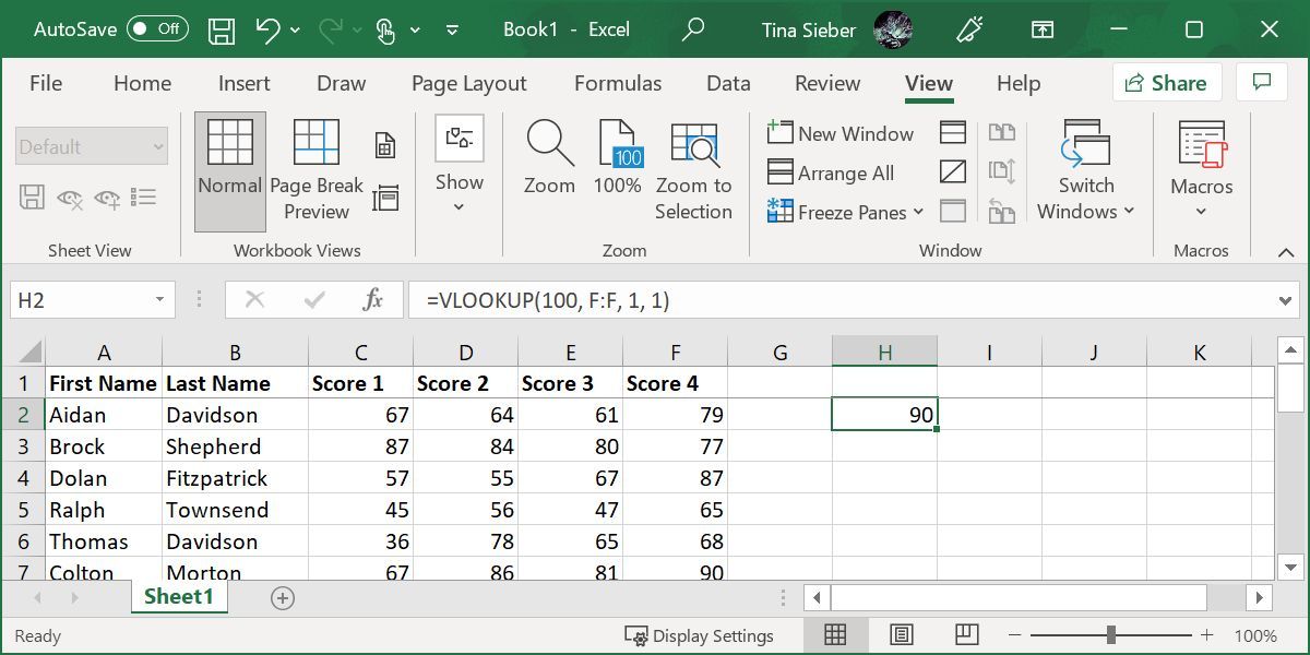
Let’s take a look at how you might use this. This spreadsheet contains student names and scores for four different tests. Let’s say you want to find score #4 for the student with the last name «Davidson.» VLOOKUP makes it easy.

Here’s the formula you’d use:

 =VLOOKUP("Davidson

Because the fourth score is the fifth column over from the last name we’re looking for, 5 is the column index argument. Note that when you’re looking for text, setting [range_lookup] to 0 is a good idea. Without it, you can get bad results.

Here’s the result:

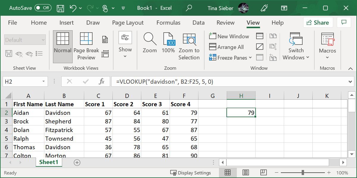
It returned 79, which is score #4 of the student we queried.

Notes on VLOOKUP

A few things are good to remember when you’re using VLOOKUP. Make sure that the first column in your range is the one that includes your lookup value. If it’s not in the first column, the function will return incorrect results. If your columns are well organized, this shouldn’t be a problem.

Also, keep in mind that VLOOKUP will only ever return one value. There was another student with the last name «Davidson,» but VLOOKUP will only ever return results for the first entry, with no indication that there is more than one match.

2. The HLOOKUP Function

Where VLOOKUP finds corresponding values in another column, HLOOKUP finds corresponding values in a different row. Because it’s usually easiest to scan through column headings until you find the right one and use a filter to find what you’re looking for, HLOOKUP is best used when you have huge spreadsheets, or if you’re working with values that are organized by time.

Here’s the syntax of the function:

 =HLOOKUP([lookup_value], [table_array], [row_index_num], [range_lookup])

[lookup_value] is the value that you know and want to find a corresponding value for.
[table_array] is the cells in which you want to search.
[row_index_num] specifies the row that the return value will come from.
[range_lookup] is the same as in VLOOKUP, leave it blank to get the nearest value when possible, or enter 0 to only look for exact matches.

We’ll use the same spreadsheet as before. You can use HLOOKUP to find the score for a specific row. Here’s how we’ll do it:

 =HLOOKUP("Score 4"

As you can see in the image below, the score is returned:

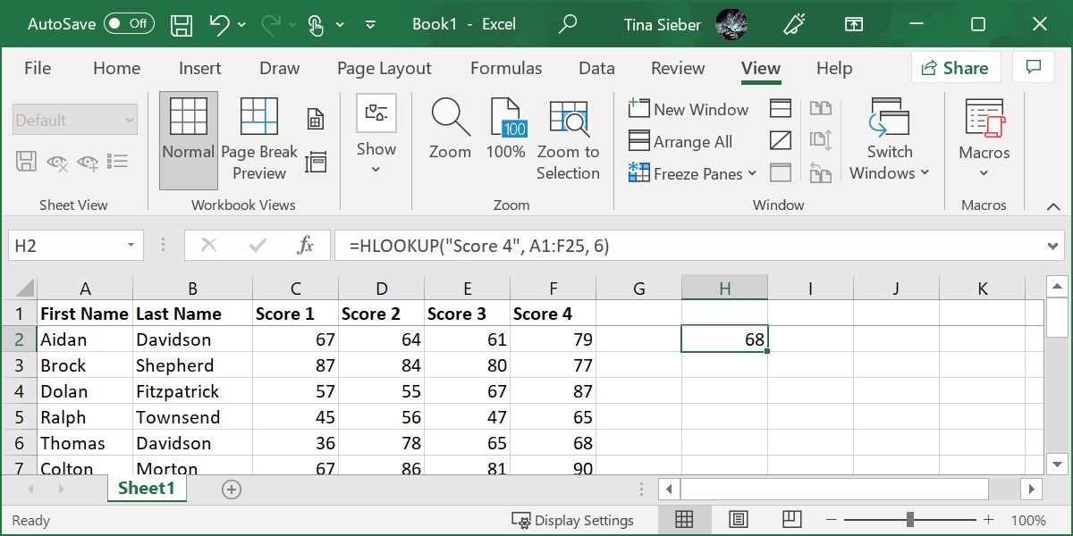
The student in row 6, Thomas Davidson, had a score of 68 on his fourth test.

Notes on HLOOKUP

As with VLOOKUP, the lookup value needs to be in the first row of your table array. This is rarely an issue with HLOOKUP, as you’ll usually be using a column title for a lookup value. HLOOKUP also only returns a single value.

3-4. The INDEX and MATCH Functions

INDEX and MATCH are two different functions, but when they’re used together, they can make searching a large spreadsheet a lot faster. Both functions have drawbacks, but by combining them, we’ll build on the strengths of both.

First, though, the syntax of both functions:

 =INDEX([array], [row_number], [column_number])

[array] is the array in which you’ll be searching.
[row_number] and [column_number] can be used to narrow your search (we’ll take a look at that in a moment).

 =MATCH([lookup_value], [lookup_array], [match_type])

[lookup_value] is a search term that can be a string or a number.
[lookup_array] is the array in which Microsoft Excel will look for the search term.
[match_type] is an optional argument that can be 1, 0, or -1. 1 will return the largest value that is smaller than or equal to your search term. 0 will only return your exact term, and -1 will return the smallest value that is greater than or equal to your search term.

It might not be clear how we’re going to use these two functions together, so I’ll lay it out here. MATCH takes a search term and returns a cell reference. In the image below, you can see that in a search for the last name «Davidson» in column B, MATCH returns 2.

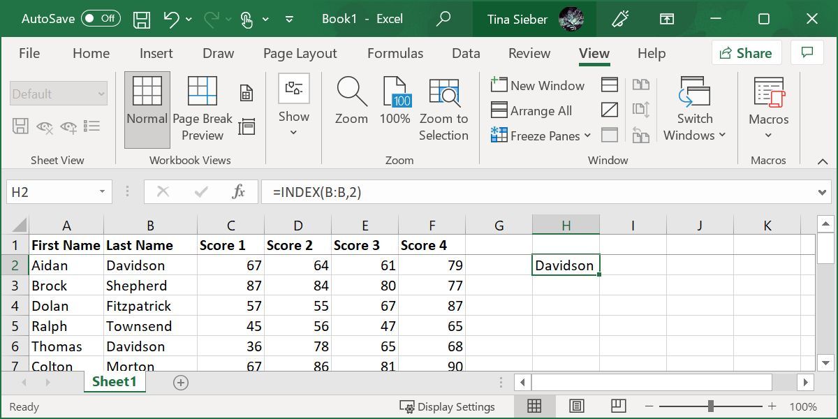
INDEX, on the other hand, does the opposite: it takes a cell reference and returns the value in it. You can see here that, when told to return the second row of column B, INDEX returns «Davidson,» the value from row 2.

What we’re going to do is combine the two so that MATCH returns a cell reference and INDEX uses that reference to look up the value in a cell. Let’s say you remember that there was a student whose last name was Townsend, and you want to see what this student’s fourth score was. Here’s the formula we’ll use:

 =INDEX(F:F, MATCH("Townsend", B:B, 0))

You’ll notice that the match type is set to 0 here. When you’re looking for a string, that’s what you’ll want to use. Here’s what we get when we run that function:

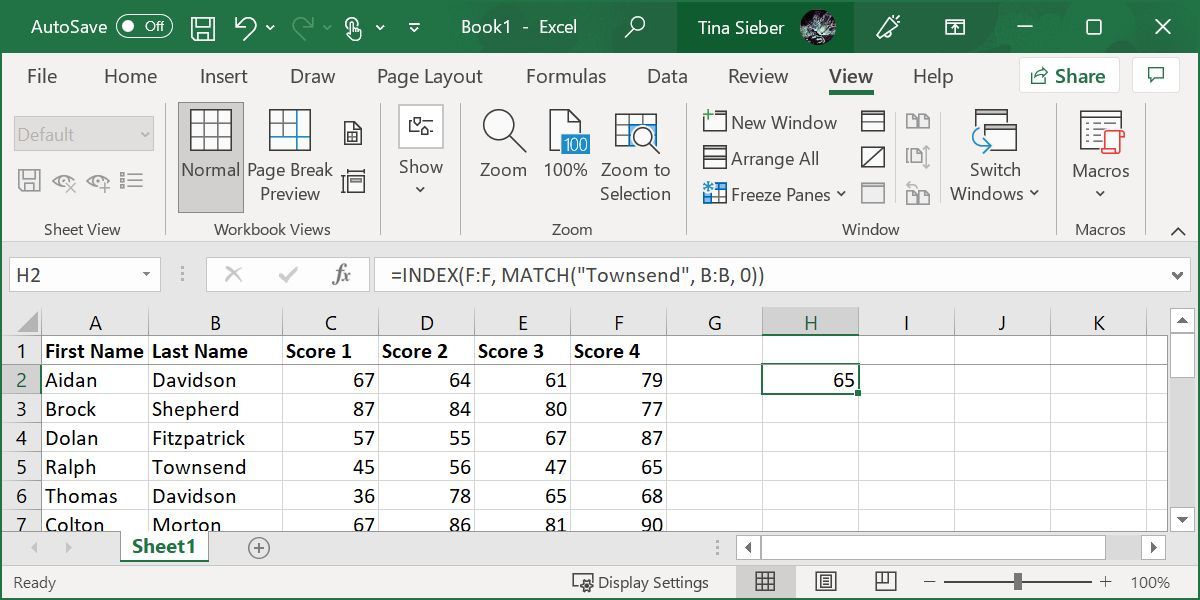
As you can see from the inset, Ralph Townsend scored a 68 in his fourth test, the number that appears when we run the function. This may not seem all that useful when you can just look a few columns over, but imagine how much time you’d save if you had to do it 50 times on a large database spreadsheet that contained several hundred columns!

5. The FIND Function

An article on finding something in Excel wouldn’t be complete without the FIND function. But it might not be what you expect. You can use Excel’s FIND function to identify the position of a string of text within another string of text.

Let’s say, we wanted to find the first occurrence of the letter «x» in the phrase «The brown fox jumped over the fence.» This would be our function:

 =FIND("x", "The brown fox jumped over the fence")

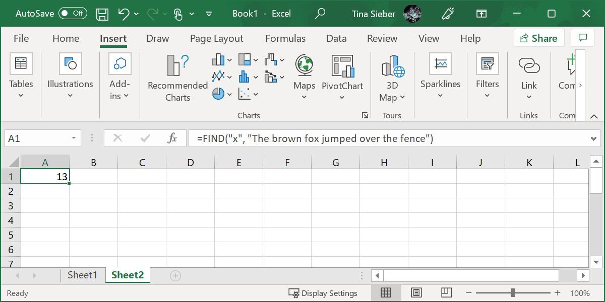
The resulting number represents the position of the queried string. If you’re looking for a multi-character string, let’s say we queried for «fox,» the result would indicate the position of the query’s first character; in this case 11.

Notes on FIND

Like VLOOKUP, HLOOKUP, and other functions, FIND will only identify the first occurrence of a string. Note that FIND is case-sensitive. You can use it to FIND multiple characters. And while we used a letter in our example, it also works with numbers.

On its own, this function might not seem very useful, but it comes into its own when you start nesting functions. For example, you could use your FIND result to split a string of text at the position corresponding to the string identified with FIND.

FIND vs. SEARCH

We can’t cover FIND without mentioning the SEARCH function. Well, it’s essentially the same as FIND, except that it’s not case-sensitive. It also allows wildcards, meaning you can search for matches that aren’t exact.

Excel supports three wildcards:

Asterisk (*), which is a placeholder for any number of characters, including zero.
Question mark (?), which can replace any one character.
Tilde (~), which turns the wildcards «asterisk» and «question mark» into literal characters, meaning it cancels their wildcard function. You’d use it as ~* or ~?.

6. The XLOOKUP Function

XLOOKUP is a new function designed to replace VLOOKUP. Like VLOOKUP, you can use it to find things in a table or range by searching for a known value. It differs from VLOOKUP in that it lets you look up values located in columns to the left or right of the queried value; with VLOOKUP you can only ever find data to the right of the queried column.

Here’s the syntax of the function:

=XLOOKUP(lookup_value, lookup_array, return_array, [if_not_found], [match_mode], [search_mode])

[lookup_value] is the value you’re searching for; i.e. your query.
[lookup_array] is the array or range to search.
[return_array] is the array or range to return. This is the first difference from VLOOKUP.
[if_not_found] is an optional argument that returns a message of your choice if no match is found.
[match_mode] is another optional argument that lets you find exact matches (0), the next smaller item (-1), the next larger item (1), or a wildcard match (2).
[search_mode] is optional and lets you control in which order to search. The default (1) starts the search at the first item. You can also start at the last item (-1), perform a binary search that depends on the lookup_array being sorted in ascending (2) or descending (-2) order.

Let’s take our VLOOKUP example and reverse the search order. This should let us find the score of the second student called Davidson. Here’s the formula:

 =XLOOKUP(G2,B2:B25,F2:F25,,,-1)

Note that we’re pulling the name from column G2, rather than writing it directly into the formula. Below is what it looks like.

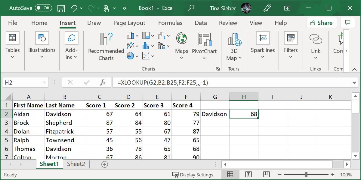
This time, the formula returned Thomas Davidson’s score, rather than that of Aidan Davidson. But it still can’t return more than one result.

Let the Excel Searches Begin

Microsoft Excel has a lot of extremely powerful functions for manipulating data, and the four listed above just scratch the surface. Learning how to use them will make your life much easier.

Источник