
Excel for Microsoft 365 Excel for Microsoft 365 for Mac Excel for the web Excel 2021 Excel 2021 for Mac Excel 2019 Excel 2019 for Mac Excel 2016 Excel 2016 for Mac Excel 2013 Excel 2010 Excel 2007 Excel for Mac 2011 Excel Starter 2010 More…Less
This article describes the formula syntax and usage of the FIND and FINDB functions in Microsoft Excel.
Description
FIND and FINDB locate one text string within a second text string, and return the number of the starting position of the first text string from the first character of the second text string.
Important:
-
These functions may not be available in all languages.
-
FIND is intended for use with languages that use the single-byte character set (SBCS), whereas FINDB is intended for use with languages that use the double-byte character set (DBCS). The default language setting on your computer affects the return value in the following way:
-
FIND always counts each character, whether single-byte or double-byte, as 1, no matter what the default language setting is.
-
FINDB counts each double-byte character as 2 when you have enabled the editing of a language that supports DBCS and then set it as the default language. Otherwise, FINDB counts each character as 1.
The languages that support DBCS include Japanese, Chinese (Simplified), Chinese (Traditional), and Korean.
Syntax
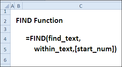
FIND(find_text, within_text, [start_num])
FINDB(find_text, within_text, [start_num])
The FIND and FINDB function syntax has the following arguments:
-
Find_text Required. The text you want to find.
-
Within_text Required. The text containing the text you want to find.
-
Start_num Optional. Specifies the character at which to start the search. The first character in within_text is character number 1. If you omit start_num, it is assumed to be 1.
Remarks
-
FIND and FINDB are case sensitive and don’t allow wildcard characters. If you don’t want to do a case sensitive search or use wildcard characters, you can use SEARCH and SEARCHB.
-
If find_text is «» (empty text), FIND matches the first character in the search string (that is, the character numbered start_num or 1).
-
Find_text cannot contain any wildcard characters.
-
If find_text does not appear in within_text, FIND and FINDB return the #VALUE! error value.
-
If start_num is not greater than zero, FIND and FINDB return the #VALUE! error value.
-
If start_num is greater than the length of within_text, FIND and FINDB return the #VALUE! error value.
-
Use start_num to skip a specified number of characters. Using FIND as an example, suppose you are working with the text string «AYF0093.YoungMensApparel». To find the number of the first «Y» in the descriptive part of the text string, set start_num equal to 8 so that the serial-number portion of the text is not searched. FIND begins with character 8, finds find_text at the next character, and returns the number 9. FIND always returns the number of characters from the start of within_text, counting the characters you skip if start_num is greater than 1.
Examples
Copy the example data in the following table, and paste it in cell A1 of a new Excel worksheet. For formulas to show results, select them, press F2, and then press Enter. If you need to, you can adjust the column widths to see all the data.
|
Data |
||
|
Miriam McGovern |
||
|
Formula |
Description |
Result |
|
=FIND(«M»,A2) |
Position of the first «M» in cell A2 |
1 |
|
=FIND(«m»,A2) |
Position of the first «M» in cell A2 |
6 |
|
=FIND(«M»,A2,3) |
Position of the first «M» in cell A2, starting with the third character |
8 |
Example 2
|
Data |
||
|
Ceramic Insulators #124-TD45-87 |
||
|
Copper Coils #12-671-6772 |
||
|
Variable Resistors #116010 |
||
|
Formula |
Description (Result) |
Result |
|
=MID(A2,1,FIND(» #»,A2,1)-1) |
Extracts text from position 1 to the position of «#» in cell A2 (Ceramic Insulators) |
Ceramic Insulators |
|
=MID(A3,1,FIND(» #»,A3,1)-1) |
Extracts text from position 1 to the position of «#» in cell A3 (Copper Coils) |
Copper Coils |
|
=MID(A4,1,FIND(» #»,A4,1)-1) |
Extracts text from position 1 to the position of «#» in cell A4 (Variable Resistors) |
Variable Resistors |
Need more help?
Want more options?
Explore subscription benefits, browse training courses, learn how to secure your device, and more.
Communities help you ask and answer questions, give feedback, and hear from experts with rich knowledge.
Содержание
- FIND, FINDB functions
- Description
- Syntax
- Remarks
- Examples
- Use Excel built-in functions to find data in a table or a range of cells
- Summary
- Create the Sample Worksheet
- Term Definitions
- Functions
- LOOKUP()
- VLOOKUP()
- INDEX() and MATCH()
- OFFSET() and MATCH()
- FIND Function
- Related functions
- Summary
- Purpose
- Return value
- Arguments
- Syntax
- Usage notes
- Basic Example
- Case-sensitive
- TRUE or FALSE result
- Start number
- Wildcards
- If cell contains
- Excel FIND and SEARCH functions with formula examples
- Excel FIND function
- Excel FIND function — things to remember!
- Excel SEARCH function
- Excel FIND vs. Excel SEARCH
- 1. Case-sensitive FIND vs. case-insensitive SEARCH
- 2. Search with wildcard characters
- Excel FIND and SEARCH formula examples
- Example 1. Find a string preceding or following a given character
- Example 2. Find Nth occurrence of a given character in a text string
- Example 3. Extract N characters following a certain character
- Example 4. Find text between parentheses
FIND, FINDB functions
This article describes the formula syntax and usage of the FIND and FINDB functions in Microsoft Excel.
Description
FIND and FINDB locate one text string within a second text string, and return the number of the starting position of the first text string from the first character of the second text string.
These functions may not be available in all languages.
FIND is intended for use with languages that use the single-byte character set (SBCS), whereas FINDB is intended for use with languages that use the double-byte character set (DBCS). The default language setting on your computer affects the return value in the following way:
FIND always counts each character, whether single-byte or double-byte, as 1, no matter what the default language setting is.
FINDB counts each double-byte character as 2 when you have enabled the editing of a language that supports DBCS and then set it as the default language. Otherwise, FINDB counts each character as 1.
The languages that support DBCS include Japanese, Chinese (Simplified), Chinese (Traditional), and Korean.
Syntax
FIND(find_text, within_text, [start_num])
FINDB(find_text, within_text, [start_num])
The FIND and FINDB function syntax has the following arguments:
Find_text Required. The text you want to find.
Within_text Required. The text containing the text you want to find.
Start_num Optional. Specifies the character at which to start the search. The first character in within_text is character number 1. If you omit start_num, it is assumed to be 1.
FIND and FINDB are case sensitive and don’t allow wildcard characters. If you don’t want to do a case sensitive search or use wildcard characters, you can use SEARCH and SEARCHB.
If find_text is «» (empty text), FIND matches the first character in the search string (that is, the character numbered start_num or 1).
Find_text cannot contain any wildcard characters.
If find_text does not appear in within_text, FIND and FINDB return the #VALUE! error value.
If start_num is not greater than zero, FIND and FINDB return the #VALUE! error value.
If start_num is greater than the length of within_text, FIND and FINDB return the #VALUE! error value.
Use start_num to skip a specified number of characters. Using FIND as an example, suppose you are working with the text string «AYF0093.YoungMensApparel». To find the number of the first «Y» in the descriptive part of the text string, set start_num equal to 8 so that the serial-number portion of the text is not searched. FIND begins with character 8, finds find_text at the next character, and returns the number 9. FIND always returns the number of characters from the start of within_text, counting the characters you skip if start_num is greater than 1.
Examples
Copy the example data in the following table, and paste it in cell A1 of a new Excel worksheet. For formulas to show results, select them, press F2, and then press Enter. If you need to, you can adjust the column widths to see all the data.
Источник
Use Excel built-in functions to find data in a table or a range of cells
Summary
This step-by-step article describes how to find data in a table (or range of cells) by using various built-in functions in Microsoft Excel. You can use different formulas to get the same result.
Create the Sample Worksheet
This article uses a sample worksheet to illustrate Excel built-in functions. Consider the example of referencing a name from column A and returning the age of that person from column C. To create this worksheet, enter the following data into a blank Excel worksheet.
You will type the value that you want to find into cell E2. You can type the formula in any blank cell in the same worksheet.
Term Definitions
This article uses the following terms to describe the Excel built-in functions:
The whole lookup table
The value to be found in the first column of Table_Array.
Lookup_Array
-or-
Lookup_Vector
The range of cells that contains possible lookup values.
The column number in Table_Array the matching value should be returned for.
3 (third column in Table_Array)
Result_Array
-or-
Result_Vector
A range that contains only one row or column. It must be the same size as Lookup_Array or Lookup_Vector.
A logical value (TRUE or FALSE). If TRUE or omitted, an approximate match is returned. If FALSE, it will look for an exact match.
This is the reference from which you want to base the offset. Top_Cell must refer to a cell or range of adjacent cells. Otherwise, OFFSET returns the #VALUE! error value.
This is the number of columns, to the left or right, that you want the upper-left cell of the result to refer to. For example, «5» as the Offset_Col argument specifies that the upper-left cell in the reference is five columns to the right of reference. Offset_Col can be positive (which means to the right of the starting reference) or negative (which means to the left of the starting reference).
Functions
LOOKUP()
The LOOKUP function finds a value in a single row or column and matches it with a value in the same position in a different row or column.
The following is an example of LOOKUP formula syntax:
The following formula finds Mary’s age in the sample worksheet:
The formula uses the value «Mary» in cell E2 and finds «Mary» in the lookup vector (column A). The formula then matches the value in the same row in the result vector (column C). Because «Mary» is in row 4, LOOKUP returns the value from row 4 in column C (22).
NOTE: The LOOKUP function requires that the table be sorted.
For more information about the LOOKUP function, click the following article number to view the article in the Microsoft Knowledge Base:
VLOOKUP()
The VLOOKUP or Vertical Lookup function is used when data is listed in columns. This function searches for a value in the left-most column and matches it with data in a specified column in the same row. You can use VLOOKUP to find data in a sorted or unsorted table. The following example uses a table with unsorted data.
The following is an example of VLOOKUP formula syntax:
The following formula finds Mary’s age in the sample worksheet:
The formula uses the value «Mary» in cell E2 and finds «Mary» in the left-most column (column A). The formula then matches the value in the same row in Column_Index. This example uses «3» as the Column_Index (column C). Because «Mary» is in row 4, VLOOKUP returns the value from row 4 in column C (22).
For more information about the VLOOKUP function, click the following article number to view the article in the Microsoft Knowledge Base:
INDEX() and MATCH()
You can use the INDEX and MATCH functions together to get the same results as using LOOKUP or VLOOKUP.
The following is an example of the syntax that combines INDEX and MATCH to produce the same results as LOOKUP and VLOOKUP in the previous examples:
The following formula finds Mary’s age in the sample worksheet:
The formula uses the value «Mary» in cell E2 and finds «Mary» in column A. It then matches the value in the same row in column C. Because «Mary» is in row 4, the formula returns the value from row 4 in column C (22).
NOTE: If none of the cells in Lookup_Array match Lookup_Value («Mary»), this formula will return #N/A.
For more information about the INDEX function, click the following article number to view the article in the Microsoft Knowledge Base:
OFFSET() and MATCH()
You can use the OFFSET and MATCH functions together to produce the same results as the functions in the previous example.
The following is an example of syntax that combines OFFSET and MATCH to produce the same results as LOOKUP and VLOOKUP:
This formula finds Mary’s age in the sample worksheet:
The formula uses the value «Mary» in cell E2 and finds «Mary» in column A. The formula then matches the value in the same row but two columns to the right (column C). Because «Mary» is in column A, the formula returns the value in row 4 in column C (22).
For more information about the OFFSET function, click the following article number to view the article in the Microsoft Knowledge Base:
Источник
FIND Function

Summary
The Excel FIND function returns the position (as a number) of one text string inside another. When the text is not found, FIND returns a #VALUE error.
Purpose
Return value
Arguments
- find_text — The substring to find.
- within_text — The text to search within.
- start_num — [optional] The starting position in the text to search. Optional, defaults to 1.
Syntax
Usage notes
The FIND function returns the position (as a number) of one text string inside another. If there is more than one occurrence of the search string, FIND returns the position of the first occurrence. When the text is not found, FIND returns a #VALUE error. Also note, when find_text is empty, FIND returns 1. FIND does not support wildcards, and is always case-sensitive. Use the SEARCH function to find the position of text without case-sensitivity and with wildcard support.
Basic Example
The FIND function is designed to look inside a text string for a specific substring. When FIND locates the substring, it returns a position of the substring in the text as a number. If the substring is not found, FIND returns a #VALUE error. For example:
Note that text values entered directly into FIND must be enclosed in double-quotes («»).
Case-sensitive
The FIND function always case-sensitive:
TRUE or FALSE result
To force a TRUE or FALSE result, nest the FIND function inside the ISNUMBER function. ISNUMBER returns TRUE for numeric values and FALSE for anything else. If FIND locates the substring, it returns the position as a number, and ISNUMBER returns TRUE:
If FIND doesn’t locate the substring, it returns an error, and ISNUMBER returns FALSE.
Start number
The FIND function has an optional argument called start_num, that controls where FIND should begin looking for a substring. To find the first match of «the» in any combination of upper or lowercase, you can omit start_num, which defaults to 1:
To start searching at character 5, enter 4 for start_num:
Wildcards
The FIND function does not support wildcards. See the SEARCH function.
If cell contains
To return a custom result with the SEARCH function, use the IF function like this:
Instead of returning TRUE or FALSE, the formula above will return «Yes» if substring is found and «No» if not.
Источник
Excel FIND and SEARCH functions with formula examples
 by Svetlana Cheusheva, updated on February 7, 2023
The tutorial explains the syntax of the Excel FIND and SEARCH functions and provides formula examples of advanced non-trivial uses.
In the last article, we covered the basics of the Excel Find and Replace dialog. In many situations, however, you may want Excel to find and extract data from other cells automatically based on your criteria. So, let’s have a closer look at what the Excel search functions have to offer.
Excel FIND function
The FIND function in Excel is used to return the position of a specific character or substring within a text string.
The syntax of the Excel Find function is as follows:
The first 2 arguments are required, the last one is optional.
- Find_text — the character or substring you want to find.
- Within_text — the text string to be searched within. Usually it’s supplied as a cell reference, but you can also type the string directly in the formula.
- Start_num — an optional argument that specifies from which character the search shall begin. If omitted, the search starts from the 1 st character of the within_text string.
If the FIND function does not find the find_text character(s), a #VALUE! error is returned.
For example, the formula =FIND(«d», «find») returns 4 because «d» is the 4 th letter in the word «find«. The formula =FIND(«a», «find») returns an error because there is no «a» in «find«. 
Excel FIND function — things to remember!
To correctly use a FIND formula in Excel, keep in mind the following simple facts:
- The FIND function is case sensitive. If you are looking for a case-insensitive match, use the SEARCH function.
- The FIND function in Excel does not allow using wildcard characters.
- If the find_text argument contains several characters, the FIND function returns the position of the first character. For example, the formula FIND(«ap»,»happy») returns 2 because «a» in the 2 nd letter in the word «happy».
- If within_text contains several occurrences of find_text, the first occurrence is returned. For example, FIND(«l», «hello») returns 3, which is the position of the first «l» character in the word «hello».
- If find_text is an empty string «», the Excel FIND formula returns the first character in the search string.
- The Excel FIND function returns the #VALUE! error if any of the following occurs:
- Find_text does not exist in within_text.
- Start_num contains more characters than within_text.
- Start_num is 0 (zero) or a negative number.
Excel SEARCH function
The SEARCH function in Excel is very similar to FIND in that it also returns the location of a substring in a text string. Is syntax and arguments are akin to those of FIND:
Unlike FIND, the SEARCH function is case-insensitive and it allows using the wildcard characters, as demonstrated in the following example.
And here’s a couple of basic Excel SEARCH formulas:
=SEARCH(«market», «supermarket») returns 6 because the substring «market» begins at the 6 th character of the word «supermarket».
=SEARCH(«e», «Excel») returns 1 because «e» is the first character in the word «Excel», ignoring the case.
Like FIND, Excel’s SEARCH function returns the #VALUE! error if:
- The value of the find_text argument is not found.
- The start_num argument is greater than the length of within_text.
- Start_num is equal to or less than zero.

Further on in this tutorial, you will find a few more meaningful formula examples that demonstrate how to use SEARCH function in Excel worksheets.
Excel FIND vs. Excel SEARCH
As already mentioned, the FIND and SEARCH functions in Excel are very much alike in terms of syntax and uses. However, they do have a couple of differences.
1. Case-sensitive FIND vs. case-insensitive SEARCH
The most essential difference between the Excel SEARCH and FIND functions is that SEARCH is case-insensitive, while FIND is case-sensitive.
For example, SEARCH(«e», «Excel») returns 1 because it ignores the case of «E», while FIND(«e», «Excel») returns 4 because it minds the case. 
2. Search with wildcard characters
Unlike FIND, the Excel SEARCH function accepts wildcard characters in the find_text argument:
- A question mark (?) matches one character, and
- An asterisk (*) matches any series of characters.
To see how it works on real data, consider the following example: 
As you see in the screenshot above, the formula SEARCH(«function*2013», A2) returns the position of the first character («f») in the substring if the text string referred to in the within_text argument contains both «function» and «2013», no matter how many other characters there are in between.
Tip. To find an actual question mark (?) or asterisk (*), type a tilde (
) before the corresponding character.
Excel FIND and SEARCH formula examples
In practice, the Excel FIND and SEARCH functions are rarely used on their own. Typically, you would utilize them in combination with other functions such as MID, LEFT or RIGHT, and the following formula examples demonstrate some real-life uses.
Example 1. Find a string preceding or following a given character
This example shows how you can find and extract all characters in a text string to the left or to the right of a specific character. To make things easier to understand, consider the following example.
Supposing you have a column of names (column A) and you want to pull the First name and Last name into separate columns.
To get the first name, you can use FIND (or SEARCH) in conjunction with the LEFT function:
=LEFT(A2, FIND(» «, A2)-1)
=LEFT(A2, SEARCH(» «, A2)-1)
As you probably know, the Excel LEFT function returns the specified number of left-most characters in a string. And you use the FIND function to determine the position of a space (» «) to let the LEFT function know how many characters to extract. At that, you subtract 1 from the space’s position because you don’t want the returned value to include the space.
To extract the last name, use the combination of the RIGHT, FIND / SEARCH and LEN functions. The LEN function is needed to get the total number of characters in the string, from which you subtract the position of the space:
The following screenshot demonstrates the result: 
For more complex scenarios, such as extracting a middle name or splitting names with suffixes, please see How to split cells in Excel using formulas.
Example 2. Find Nth occurrence of a given character in a text string
Supposing you have some text strings in column A, say a list of SKUs, and you want to find the position of the 2 nd dash in a string. The following formula works a treat:
The first two arguments are easy to interpret: locate a dash («-«) in cell A2. In the third argument (start_num), you embed another FIND function that tells Excel to start searching beginning with the character that comes right after the first occurrence of dash (FIND(«-«,A2)+1).
To return the position of the 3 rd occurrence, you embed the above formula in the start_num argument of another FIND function and add 2 to the returned value:
=FIND(«-«,A2, FIND(«-«, A2, FIND(«-«,A2)+1) +2) 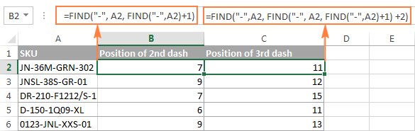
Another and probably a simpler way of finding the Nth occurrence of a given character is using the Excel FIND function in combination with CHAR and SUBSTITUTE:
Where «-» is the character in question and «3» is the Nth occurrence you want to find.
In the above formula, the SUBSTITUTE function replaces the 3rd occurrence of dash («-«) with CHAR(1), which is the unprintable «Start of Heading» character in the ASCII system. Instead of CHAR(1) you can use any other unprintable character from 1 to 31. And then, the FIND function returns the position of that character in the text string. So, the general formula is as follows:
At first sight, it may seem that the above formulas have little practical value, but the next example will show how useful they are in solving real tasks.
Note. Please remember that the Excel FIND function is case-sensitive. In our example, this makes no difference, but if you are working with letters and you want a case-insensitive match, use the SEARCH function instead of FIND.
To locate a substring of a given length within any text string, use Excel FIND or Excel SEARCH in combination with the MID function. The following example demonstrates how you can use such formulas in practice.
In our list of SKUs, supposing you want to find the first 3 characters following the first dash and pull them in another column.
If the group of characters preceding the first dash always contains the same number of items (e.g. 2 chars) this would be a trivial task. You could use the MID function to return 3 characters from a string, starting at position 4 (skipping the first 2 characters and a dash):
Translated into English, the formula says: «Look in cell A2, begin extracting from character 4, and return 3 characters». 
However, in real-life worksheets, the substring you need to extract could start anywhere within the text string. In our example, you may not know how many characters precede the first dash. To cope with this challenge, use the FIND function to determine the starting point of the substring that you want to retrieve.
The FIND formula to return the position of the 1 st dash is as follows:
Because you want to start with the character that follows the dash, add 1 to the returned value and embed the above function in the second argument (start_num) of the MID function:
In this scenario, the Excel SEARCH function works equally well:
=MID(A2, SEARCH(«-«,A2)+1, 3) 
It’s great, but what if the group of chars following the first dash contains a different number of characters? Hmm. this might be a problem: 
As you see in the above screenshot, the formula works perfectly for rows 1 and 2. In rows 4 and 5, the second group contains 4 characters, but only the first 3 chars are returned. In rows 6 and 7, there are only 2 characters in the second group, and therefore our Excel Search formula returns a dash following them.
If you wanted to return all chars between the 1 st and 2 nd occurrences of a certain character (dash in this example), how would you proceed? Here is the answer:
=MID(A2, FIND(«-«,A2)+1, FIND(«-«, A2, FIND(«-«,A2)+1) — FIND(«-«,A2)-1) 
For better understanding of this MID formula, let’s examine its arguments one by one:
- 1 st argument (text). It’s the text string containing the characters you want to extract, cell A2 in this example.
- 2 nd argument (start_position). Specifies the position of the first character you want to extract. You use the FIND function to locate the first dash in the string and add 1 to that value because you want to start with the character that follows the dash: FIND(«-«,A2)+1.
- 3 rd argument (num_chars). Specifies the number of characters you want to return. In our formula, this is the trickiest part. You use two FIND (or SEARCH) functions, one determines the position of the first dash: FIND(«-«,A2). And the other returns the position of the second dash: FIND(«-«, A2, FIND(«-«,A2)+1). Then you subtract the former from the latter, and then subtract 1 because you don’t want to include either dash. As the result, you will get the number of characters between the 1 st and 2 nd dashes, which is exactly what we are looking for. So, you feed that value to the num_chars argument of the MID function.
In a similar fashion, you can return 3 characters after the 2 nd dash:
=MID(A2, FIND(«-«,A2, FIND(«-«, A2, FIND(«-«,A2)+1) +2), 3)
Or, extract all the characters between the 2 nd and 3 rd dashes:
=MID(A2, FIND(«-«, A2, FIND(«-«,A2)+1)+1, FIND(«-«,A2, FIND(«-«, A2, FIND(«-«,A2)+1) +2) — FIND(«-«, A2, FIND(«-«,A2)+1)-1) 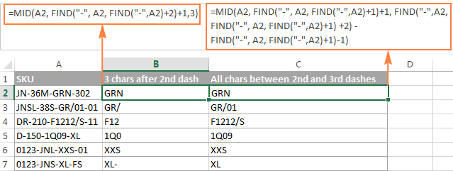
Example 4. Find text between parentheses
Supposing you have some long text string in column A and you want to find and extract only the text enclosed in (parentheses).
To do this, you would need the MID function to return the desired number of characters from a string, and either Excel FIND or SEARCH function to determine where to start and how many characters to extract.
The logic of this formula is similar to the ones we discussed in the previous example. And again, the most complex part is the last argument that tells the formula how many characters to return. That pretty long expression in the num_chars argument does the following:
- First, you find the position of the closing parenthesis: SEARCH(«)»,A2)
- After that you locate the position of the opening parenthesis: SEARCH(«(«,A2)
- And then, you calculate the difference between the positions of the closing and opening parentheses and subtract 1 from that number, because you don’t want either parenthesis in the result: SEARCH(«)»,A2)-SEARCH(«(«,A2))-1

Naturally, nothing prevents you from using the Excel FIND function instead of SEARCH, because case-sensitivity or case-insensitivity makes no difference in this example.
Hopefully, this tutorial has shed some light on how to use SEARCH and FIND functions in Excel. In the next tutorial, we are going to closely examine the REPLACE function, so please stay tuned. Thank you for reading!
Источник
Purpose
Get location substring in a string
Return value
A number representing the location of substring
Usage notes
The FIND function returns the position (as a number) of one text string inside another. If there is more than one occurrence of the search string, FIND returns the position of the first occurrence. When the text is not found, FIND returns a #VALUE error. Also note, when find_text is empty, FIND returns 1. FIND does not support wildcards, and is always case-sensitive. Use the SEARCH function to find the position of text without case-sensitivity and with wildcard support.
Basic Example
The FIND function is designed to look inside a text string for a specific substring. When FIND locates the substring, it returns a position of the substring in the text as a number. If the substring is not found, FIND returns a #VALUE error. For example:
=FIND("p","apple") // returns 2
=FIND("z","apple") // returns #VALUE!
Note that text values entered directly into FIND must be enclosed in double-quotes («»).
Case-sensitive
The FIND function always case-sensitive:
=FIND("a","Apple") // returns #VALUE!
=FIND("A","Apple") // returns 1
TRUE or FALSE result
To force a TRUE or FALSE result, nest the FIND function inside the ISNUMBER function. ISNUMBER returns TRUE for numeric values and FALSE for anything else. If FIND locates the substring, it returns the position as a number, and ISNUMBER returns TRUE:
=ISNUMBER(FIND("p","apple")) // returns TRUE
=ISNUMBER(FIND("z","apple")) // returns FALSE
If FIND doesn’t locate the substring, it returns an error, and ISNUMBER returns FALSE.
Start number
The FIND function has an optional argument called start_num, that controls where FIND should begin looking for a substring. To find the first match of «the» in any combination of upper or lowercase, you can omit start_num, which defaults to 1:
=FIND("x","20 x 30 x 50") // returns 4To start searching at character 5, enter 4 for start_num:
=FIND("x","20 x 30 x 50",5) // returns 9
Wildcards
The FIND function does not support wildcards. See the SEARCH function.
If cell contains
To return a custom result with the SEARCH function, use the IF function like this:
=IF(ISNUMBER(FIND(substring,A1)), "Yes", "No")
Instead of returning TRUE or FALSE, the formula above will return «Yes» if substring is found and «No» if not.
Notes
- The FIND function returns the location of the first find_text in within_text.
- The location is returned as the number of characters from the start.
- Start_num is optional and defaults to 1.
- FIND returns 1 when find_text is empty.
- FIND returns #VALUE if find_text is not found.
- FIND is case-sensitive but does not support wildcards.
- Use the SEARCH function to find a substring with wildcards.
|
Функция производит поиск текстового значения в заданном диапазоне листа, Взято с сайта Чипа Пирсона: cpearson.com/excel/FindAll.aspx Function FindAll(SearchRange As Range, _ FindWhat As Variant, _ Optional LookIn As XlFindLookIn = xlValues, _ Optional LookAt As XlLookAt = xlWhole, _ Optional SearchOrder As XlSearchOrder = xlByRows, _ Optional MatchCase As Boolean = False, _ Optional BeginsWith As String = vbNullString, _ Optional EndsWith As String = vbNullString, _ Optional BeginEndCompare As VbCompareMethod = vbTextCompare) As Range ''''''''''''''''''''''''''''''''''''''''''''''''''''''''''''''''''''''''''''''''''''' ' FindAll ' This searches the range specified by SearchRange and returns a Range object ' that contains all the cells in which FindWhat was found. The search parameters to ' this function have the same meaning and effect as they do with the ' Range.Find method. If the value was not found, the function return Nothing. If ' BeginsWith is not an empty string, only those cells that begin with BeginWith ' are included in the result. If EndsWith is not an empty string, only those cells ' that end with EndsWith are included in the result. Note that if a cell contains ' a single word that matches either BeginsWith or EndsWith, it is included in the ' result. If BeginsWith or EndsWith is not an empty string, the LookAt parameter ' is automatically changed to xlPart. The tests for BeginsWith and EndsWith may be ' case-sensitive by setting BeginEndCompare to vbBinaryCompare. For case-insensitive ' comparisons, set BeginEndCompare to vbTextCompare. If this parameter is omitted, ' it defaults to vbTextCompare. The comparisons for BeginsWith and EndsWith are ' in an OR relationship. That is, if both BeginsWith and EndsWith are provided, ' a match if found if the text begins with BeginsWith OR the text ends with EndsWith. ''''''''''''''''''''''''''''''''''''''''''''''''''''''''''''''''''''''''''''''''''''' Dim FoundCell As Range, FirstFound As Range, LastCell As Range, rngResultRange As Range Dim XLookAt As XlLookAt, Include As Boolean, CompMode As VbCompareMethod Dim Area As Range, MaxRow As Long, MaxCol As Long, BeginB As Boolean, EndB As Boolean CompMode = BeginEndCompare XLookAt = LookAt: If BeginsWith <> vbNullString Or EndsWith <> vbNullString Then XLookAt = xlPart ' this loop in Areas is to find the last cell of all the areas. That is, the cell whose row ' and column are greater than or equal to any cell in any Area. For Each Area In SearchRange.Areas With Area If .Cells(.Cells.Count).Row > MaxRow Then MaxRow = .Cells(.Cells.Count).Row If .Cells(.Cells.Count).Column > MaxCol Then MaxCol = .Cells(.Cells.Count).Column End With Next Area Set LastCell = SearchRange.Worksheet.Cells(MaxRow, MaxCol) Set FoundCell = SearchRange.Find(what:=FindWhat, after:=LastCell, _ LookIn:=LookIn, LookAt:=XLookAt, _ SearchOrder:=SearchOrder, MatchCase:=MatchCase) If Not FoundCell Is Nothing Then Set FirstFound = FoundCell Do Until False ' Loop forever. We'll "Exit Do" when necessary. Include = False If BeginsWith = vbNullString And EndsWith = vbNullString Then Include = True Else If BeginsWith <> vbNullString Then If StrComp(Left(FoundCell.Text, Len(BeginsWith)), _ BeginsWith, BeginEndCompare) = 0 Then Include = True End If If EndsWith <> vbNullString Then If StrComp(Right(FoundCell.Text, Len(EndsWith)), _ EndsWith, BeginEndCompare) = 0 Then Include = True End If End If If Include = True Then If rngResultRange Is Nothing Then Set rngResultRange = FoundCell Else Set rngResultRange = Application.Union(rngResultRange, FoundCell) End If End If Set FoundCell = SearchRange.FindNext(after:=FoundCell) If (FoundCell Is Nothing) Then Exit Do If (FoundCell.Address = FirstFound.Address) Then Exit Do Loop End If Set FindAll = rngResultRange End Function
Не получается применить макрос? Не удаётся изменить код под свои нужды? Оформите заказ у нас на сайте, не забыв прикрепить примеры файлов, и описать, что и как должно работать. |
Вчера в марафоне 30 функций Excel за 30 дней у нас был разгрузочный день с функцией N (Ч), где мы выяснили, что она может возвратить число, основываясь на типе содержимого ячейки.
23-й день марафона мы посвятим изучению функции FIND (НАЙТИ). Она очень похожа на функцию SEARCH (ПОИСК), с которой мы встречались ранее, но функция FIND (НАЙТИ) чувствительна к регистру.
Итак, давайте посмотрим сведения и примеры по функции FIND (НАЙТИ). Если у Вас есть дополнительная информация или примеры, пожалуйста, делитесь ими в комментариях.
Содержание
- Функция 23: FIND (НАЙТИ)
- Как можно использовать функцию FIND (НАЙТИ)?
- Синтаксис FIND (НАЙТИ)
- Ловушки FIND (НАЙТИ)
- Пример 1: Находим текст в текстовой строке
- Пример 2: Находим точные значения на листе
- Пример 3: Находим название улицы в адресе
Функция 23: FIND (НАЙТИ)
Функция FIND (НАЙТИ) находит текстовую строку внутри другой текстовой строки с учётом регистра.
Как можно использовать функцию FIND (НАЙТИ)?
Функция FIND (НАЙТИ) может найти текст внутри текстовой строки, учитывая регистр символов. Например:
- Найти начальную позицию текста в текстовой строке.
- Найти точные данные на листе.
- Найти название улицы в адресе.
Синтаксис FIND (НАЙТИ)
Функция FIND (НАЙТИ) имеет вот такой синтаксис:
FIND(find_text,within_text,[start_num])
НАЙТИ(искомый_текст;просматриваемый_текст;[нач_позиция])
- find_text (искомый_текст) – текст, который Вы ищете.
- within_text (просматриваемый_текст) – текстовая строка, внутри которой происходит поиск.
- start_num (нач_позиция) – если не указан, то поиск начнётся с первого символа.
Ловушки FIND (НАЙТИ)
- Функция FIND (НАЙТИ) возвратит позицию первой совпадающей строки с учётом регистра. Для того, чтобы произвести поиск без учёта регистра, используйте функцию SEARCH (ПОИСК), которую мы уже рассматривали ранее в рамках марафона 30 функций Excel за 30 дней.
- В аргументе find_text (искомый_текст) функции FIND (НАЙТИ) нельзя использовать символы подстановки. Если Вы все-таки хотите их использовать, то применяйте функцию SEARCH (ПОИСК).
Пример 1: Находим текст в текстовой строке
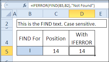
Чтобы найти нужный текст в текстовой строке, используйте функцию FIND (НАЙТИ). Она чувствительна к регистру, поэтому на рисунке ниже первые два символа «i» игнорируются.
=FIND(B5,B2)
=НАЙТИ(B5;B2)
Чтобы обработать ошибки, возникающие, если текст не найден, поместите FIND (НАЙТИ) в функцию IFERROR (ЕСЛИОШИБКА). Если у Вас Excel 2003 или более ранняя версия, вместо IFERROR (ЕСЛИОШИБКА) используйте функцию IF (ЕСЛИ) вместе с ISERROR (ЕОШИБКА).
=IFERROR(FIND(B5,B2),"Not Found")
=ЕСЛИОШИБКА(НАЙТИ(B5;B2);"Not Found")
Пример 2: Находим точные значения на листе
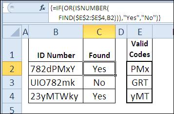
Пользуясь тем, что функция FIND (НАЙТИ) чувствительна к регистру, Вы можете использовать её для точного поиска строки текста внутри другой строки. В этом примере в столбце E записаны значения допустимых кодов (Valid Codes). При помощи функции FIND (НАЙТИ) мы можем определить содержит ли значение в ячейке B2 хотя бы один из допустимых кодов.
Эта формула должна быть введена, как формула массива, нажатием Ctrl+Shift+Enter.
=IF(OR(ISNUMBER(FIND($E$2:$E$4,B2))),"Yes","No")
=ЕСЛИ(ЕЧИСЛО(НАЙТИ($E$2:$E$4;B2)));"Yes";"No")
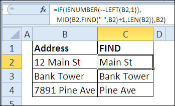
Пример 3: Находим название улицы в адресе
В следующем примере большинство адресов в столбце B начинается с номера. При помощи формулы в столбце C мы проверяем, является ли первый символ цифрой. Если это цифра, то функция FIND (НАЙТИ) находит первый символ пробела, а функция MID (ПСТР) возвращает весь оставшийся текст, начиная со следующего символа.
=IF(ISNUMBER(--LEFT(B2,1)),MID(B2,FIND(" ",B2)+1,LEN(B2)),B2)
=ЕСЛИ(ЕЧИСЛО(--ЛЕВСИМВ(B2;1));ПСТР(B2;НАЙТИ(" ";B2)+1;ДЛСТР(B2));B2)
Оцените качество статьи. Нам важно ваше мнение: