
Summary
This step-by-step article describes how to find data in a table (or range of cells) by using various built-in functions in Microsoft Excel. You can use different formulas to get the same result.
Create the Sample Worksheet
This article uses a sample worksheet to illustrate Excel built-in functions. Consider the example of referencing a name from column A and returning the age of that person from column C. To create this worksheet, enter the following data into a blank Excel worksheet.
You will type the value that you want to find into cell E2. You can type the formula in any blank cell in the same worksheet.
|
A |
B |
C |
D |
E |
||
|
1 |
Name |
Dept |
Age |
Find Value |
||
|
2 |
Henry |
501 |
28 |
Mary |
||
|
3 |
Stan |
201 |
19 |
|||
|
4 |
Mary |
101 |
22 |
|||
|
5 |
Larry |
301 |
29 |
Term Definitions
This article uses the following terms to describe the Excel built-in functions:
|
Term |
Definition |
Example |
|
Table Array |
The whole lookup table |
A2:C5 |
|
Lookup_Value |
The value to be found in the first column of Table_Array. |
E2 |
|
Lookup_Array |
The range of cells that contains possible lookup values. |
A2:A5 |
|
Col_Index_Num |
The column number in Table_Array the matching value should be returned for. |
3 (third column in Table_Array) |
|
Result_Array |
A range that contains only one row or column. It must be the same size as Lookup_Array or Lookup_Vector. |
C2:C5 |
|
Range_Lookup |
A logical value (TRUE or FALSE). If TRUE or omitted, an approximate match is returned. If FALSE, it will look for an exact match. |
FALSE |
|
Top_cell |
This is the reference from which you want to base the offset. Top_Cell must refer to a cell or range of adjacent cells. Otherwise, OFFSET returns the #VALUE! error value. |
|
|
Offset_Col |
This is the number of columns, to the left or right, that you want the upper-left cell of the result to refer to. For example, «5» as the Offset_Col argument specifies that the upper-left cell in the reference is five columns to the right of reference. Offset_Col can be positive (which means to the right of the starting reference) or negative (which means to the left of the starting reference). |
Functions
LOOKUP()
The LOOKUP function finds a value in a single row or column and matches it with a value in the same position in a different row or column.
The following is an example of LOOKUP formula syntax:
=LOOKUP(Lookup_Value,Lookup_Vector,Result_Vector)
The following formula finds Mary’s age in the sample worksheet:
=LOOKUP(E2,A2:A5,C2:C5)
The formula uses the value «Mary» in cell E2 and finds «Mary» in the lookup vector (column A). The formula then matches the value in the same row in the result vector (column C). Because «Mary» is in row 4, LOOKUP returns the value from row 4 in column C (22).
NOTE: The LOOKUP function requires that the table be sorted.
For more information about the LOOKUP function, click the following article number to view the article in the Microsoft Knowledge Base:
How to use the LOOKUP function in Excel
VLOOKUP()
The VLOOKUP or Vertical Lookup function is used when data is listed in columns. This function searches for a value in the left-most column and matches it with data in a specified column in the same row. You can use VLOOKUP to find data in a sorted or unsorted table. The following example uses a table with unsorted data.
The following is an example of VLOOKUP formula syntax:
=VLOOKUP(Lookup_Value,Table_Array,Col_Index_Num,Range_Lookup)
The following formula finds Mary’s age in the sample worksheet:
=VLOOKUP(E2,A2:C5,3,FALSE)
The formula uses the value «Mary» in cell E2 and finds «Mary» in the left-most column (column A). The formula then matches the value in the same row in Column_Index. This example uses «3» as the Column_Index (column C). Because «Mary» is in row 4, VLOOKUP returns the value from row 4 in column C (22).
For more information about the VLOOKUP function, click the following article number to view the article in the Microsoft Knowledge Base:
How to Use VLOOKUP or HLOOKUP to find an exact match
INDEX() and MATCH()
You can use the INDEX and MATCH functions together to get the same results as using LOOKUP or VLOOKUP.
The following is an example of the syntax that combines INDEX and MATCH to produce the same results as LOOKUP and VLOOKUP in the previous examples:
=INDEX(Table_Array,MATCH(Lookup_Value,Lookup_Array,0),Col_Index_Num)
The following formula finds Mary’s age in the sample worksheet:
=INDEX(A2:C5,MATCH(E2,A2:A5,0),3)
The formula uses the value «Mary» in cell E2 and finds «Mary» in column A. It then matches the value in the same row in column C. Because «Mary» is in row 4, the formula returns the value from row 4 in column C (22).
NOTE: If none of the cells in Lookup_Array match Lookup_Value («Mary»), this formula will return #N/A.
For more information about the INDEX function, click the following article number to view the article in the Microsoft Knowledge Base:
How to use the INDEX function to find data in a table
OFFSET() and MATCH()
You can use the OFFSET and MATCH functions together to produce the same results as the functions in the previous example.
The following is an example of syntax that combines OFFSET and MATCH to produce the same results as LOOKUP and VLOOKUP:
=OFFSET(top_cell,MATCH(Lookup_Value,Lookup_Array,0),Offset_Col)
This formula finds Mary’s age in the sample worksheet:
=OFFSET(A1,MATCH(E2,A2:A5,0),2)
The formula uses the value «Mary» in cell E2 and finds «Mary» in column A. The formula then matches the value in the same row but two columns to the right (column C). Because «Mary» is in column A, the formula returns the value in row 4 in column C (22).
For more information about the OFFSET function, click the following article number to view the article in the Microsoft Knowledge Base:
How to use the OFFSET function
Need more help?
Assuming we have a Sheet1 like this:

note, the Sheet1is sorted by Start_Pos, End_Pos in ascending order.
and a Sheet2 like this:

Then the formula in Sheet2!B2 downwards could be:
=INDEX(Sheet1!A:A,IF(MATCH(A2,Sheet1!B:B)>IFERROR(MATCH(A2-(10^-10),Sheet1!C:C),0),MATCH(A2,Sheet1!B:B),NA()))
See MATCH: https://support.office.com/en-us/article/MATCH-function-e8dffd45-c762-47d6-bf89-533f4a37673a
The idea is: MATCH without exact matching (without parameter match_type) gets the row of the largest value which is smaller or equal the search value. So in the Start_Pos column it will get the row from which we can get the S2_Symbol. But from the End_Pos column it should get one row beforehand if the value is not outside the given ranges.
There is only one exception. If the value is exact the value in the End_Pos column, then it will return the same row as in the Start_Pos column. Considering this exception, we can search in the End_Pos column with a little bit smaller value. Thanks to Tom Sharpe for his comment.
The formula in Sheet2!D2 downwards is:
{=INDEX(Sheet1!A:A,MIN(IF($A2>=Sheet1!$B$2:$B$300000,IF($A2<=Sheet1!$C$2:$C$300000,ROW(Sheet1!$A$2:$A$300000),2^20+1))))}
this is an array formula which is exactly formulated respecting the requirements. But this is very bad in performance for using in much many cells. But using this, the Sheet1 is not required to be sorted.
Benchmark test:
Have the following Sheet1:

Formulas:
A2:A300002: ="S"&(ROW(A1)-1)*10&"-"&(ROW(A1)-1)*10+7
B2:B300002: =(ROW(A1)-1)*10
C2:C300002: =B2+7
and the following Sheet2:

Formulas:
A2:A300002: =RANDBETWEEN(0,3000007)
B2:B300002: =INDEX(Sheet1!A:A,IF(MATCH(A2,Sheet1!B:B)>IFERROR(MATCH(A2-10^-9,Sheet1!C:C),0),MATCH(A2,Sheet1!B:B),NA()))
Note the -10^-9 instead of -10^-10 in previous version. This is because we have only 16 digits precision. In previous version this was maximum 6 digits integer part and then 10 digits decimal part. Now it is maximum 7 digits integer part and then 9 digits decimal part.
Calculation after pressing F9 in Sheet2 takes ca. 2 s. (Excel 2007, Windows 7, 4 core processor).
We usually require certain metrics to understand the data that we are working with. There are a number of such representative metrics, like the average, the median, etc. Among these metrics, an often-used value is the ‘Range’.
In this tutorial, we will show you two easy ways in which you can find the range of a series of numbers in Excel:
- Using a formula with the MIN and MAX built-in functions
- Using a formula with the SMALL and LARGE built-in functions
What is Range and How is it Calculated?
The range is a measure of the spread of values in a series. In other words, it is the variation between the upper and lower limits of the series on a particular scale.
To find the range of a set of numbers, you need to find the difference between the largest and smallest numbers.
For example, if you have a series of numbers {4,2,6,5,3} then the range can be calculated as follows:
Range = largest value - smallest value
= 6 – 2
Calculation of the range is a very simple process, requiring three basic arithmetic operations:
- Finding the largest value
- Finding the smallest value
- Finding the difference between the two
Given below are two methods to quickly calculate the range of a set of numbers in Excel. To demonstrate both methods, we will use the following dataset:

Finding the Range in Excel with MIN and MAX Functions
The first way to find the range is to use a combination of the MIN and MAX functions.
The MIN Function
The Excel MIN function returns the smallest numeric value in a range of values. The syntax for the MIN function is as follows:
=MIN (number1, [number2], ...)
Here,
- number1 can be a numeric value, a reference to a numeric value, or a range of numeric values.
- number2,… is optional. It can be a numeric value, a reference to a numeric value, or a range of numeric values.
For example, to find the minimum value of numbers in the range B2:B7, you will write the MIN function as follows:
=MIN(B2:B7)
The MAX Function
The Excel MAX function returns the largest numeric value in a range of values. The syntax for the MAX function is as follows:
=MAX (number1, [number2], ...)
Here,
- number1 can be a numeric value, a reference to a numeric value, or a range of numeric values.
- number2, … is optional. It can be a numeric value, a reference to a numeric value, or a range of numeric values.
For example, to find the maximum value of numbers in the range B2:B7, you will write the MAX function as follows:
=MAX(B2:B7)
Note: Both MIN and MAX functions ignore empty cells, logical values like TRUE and FALSE, as well as text values.
Using the MIN and MAX functions to Find the Range of A Series
To find the range of values in the given dataset, we can use the MIN and MAX functions as follows:
- Select the cell where you want to display the range (B8 in our example).
- Type in the formula: =MAX(B2:B7)-MIN(B2:B7)
- Press the Return key.

Note: You can replace the reference B2:B7 with reference to the cells containing the values you want to calculate the range for.
Explanation of the Formula
The formula simply performed the basic steps required to calculate the range:
- Finding the largest value: =MAX(B2:B7)
- Finding the smallest value: =MIN(B2:B7)
- Finding the difference between the two: =MAX(B2:B7) – MIN(B2:B7)
Finding the Range in Excel with SMALL and LARGE Functions
The second way to find the range is to use a combination of the SMALL and LARGE function.
The SMALL Function
The Excel SMALL function returns the ‘n-th smallest value’ in a range of values. So you can use it to find the 1st smallest value, 2nd smallest value, 3rd smallest value, and so on.
The syntax for the SMALL function is as follows:
=SMALL (array, n)
Here,
- array is the range of cells that you want to find the n-th smallest value from.
- n is an integer that specifies the position from the smallest value, i.e. the nth position.
For example, to find the 3rd smallest value in the range B2:B7, you will write the SMALL function as follows:
=SMALL(B2:B7,3)
Similarly, to find the smallest value in the range B2:B7, you will write the function as follows:
=SMALL(B2:B7, 1)
Notice the above function gives a result equivalent to the function:
=MIN(A2:A7)
The LARGE Function
The Excel LARGE function returns the ‘n-th largest value’ in a range of values. So you can use it to find the 1st largest value, 2nd largest value, 3rd largest value and so on.
The syntax for the LARGE function is as follows:
= LARGE (array, n)
Here,
- array is the range of cells that you want to find the n-th largest value from.
- n is an integer that specifies the position from the largest value, i.e. the nth position.
For example, to find the 3rd largest value in the range B2:B7, you will write the LARGE function as follows:
= LARGE (B2:B7,3)
Similarly, to find the largest value in the range B2:B7, you will write the function as follows:
= LARGE (B2:B7, 1)
Notice the above function gives a result equivalent to the function:
=MAX(B2:B7)
Note: In cases where you’re working with large volumes of data, using the MIN and MAX functions are more efficient to use than the SMALL and LARGE. This is because the SMALL and LARGE functions require more computing and resources.
Using the SMALL and LARGE functions to Find the Range of A Series
To find the range of values in the given dataset, we can use the SMALL and LARGE functions as follows:
- Select the cell where you want to display the range (B8 in our example).
- Type in the formula: =LARGE(B2:B7,1) – SMALL(B2:B7,1)
- Press the Return key.

Note: You can replace the reference B2:B7 with reference to the cells containing the values you want to calculate the range for.
Explanation of the Formula
The formula simply performed the basic steps required to calculate the range:
- Finding the largest value: = LARGE(B2:B7,1)
- Finding the smallest value: = SMALL(B2:B7,1)
- Finding the difference between the two: =LARGE(B2:B7,1)-SMALL(B2:B7,1)
Applications and Limitations of the Range
The range provides a great way for us to get a basic understanding of how spread out the numbers in the dataset are.
So, a higher range value means the data is quite spread out, while a smaller range value means the data is less spread out, or more concentrated.
It must be noted, though, that the range is a very crude measurement since it is quite sensitive to outliers.
A single value that is too high or too low can completely alter the range, giving an erroneous representation of the data. As such, it doesn’t always provide a true indication of the spread in the dataset.
Having said that, the range is easy to calculate. It only requires basic operations. So, it is a good way to help you get a very basic understanding of the nature of your data.
Other Excel tutorials you may also like:
- How to Calculate Standard Error In Excel
- How to Square a Number in Excel
- How to Use Pi (π) in Excel
- How to Calculate Antilog in Excel
- How to Use e in Excel | Euler’s Number in Excel
- How to Find Outliers in Excel
- How to Find Slope in Excel (Easy Formula)
- How to Find Percentile in Excel (PERCENTILE Function)
In this example, the goal is to use a formula to check if a specific value exists in a range. The easiest way to do this is to use the COUNTIF function to count occurences of a value in a range, then use the count to create a final result.
COUNTIF function
The COUNTIF function counts cells that meet supplied criteria. The generic syntax looks like this:
=COUNTIF(range,criteria)Range is the range of cells to test, and criteria is a condition that should be tested. COUNTIF returns the number of cells in range that meet the condition defined by criteria. If no cells meet criteria, COUNTIF returns zero. In the example shown, we can use COUNTIF to count the values we are looking for like this
COUNTIF(data,E5)Once the named range data (B5:B16) and cell E5 have been evaluated, we have:
=COUNTIF(data,E5)
=COUNTIF(B5:B16,"Blue")
=1
COUNTIF returns 1 because «Blue» occurs in the range B5:B16 once. Next, we use the greater than operator (>) to run a simple test to force a TRUE or FALSE result:
=COUNTIF(data,B5)>0 // returns TRUE or FALSEBy itself, the formula above will return TRUE or FALSE. The last part of the problem is to return a «Yes» or «No» result. To handle this, we nest the formula above into the IF function like this:
=IF(COUNTIF(data,E5)>0,"Yes","No")This is the formula shown in the worksheet above. As the formula is copied down, COUNTIF returns a count of the value in column E. If the count is greater than zero, the IF function returns «Yes». If the count is zero, IF returns «No».
Slightly abbreviated
It is possible to shorten this formula slightly and get the same result like this:
=IF(COUNTIF(data,E5),"Yes","No")Here, we have remove the «>0» test. Instead, we simply return the count to IF as the logical_test. This works because Excel will treat any non-zero number as TRUE when the number is evaluated as a Boolean.
Testing for a partial match
To test a range to see if it contains a substring (a partial match), you can add a wildcard to the formula. For example, if you have a value to look for in cell C1, and you want to check the range A1:A100 for partial matches, you can configure COUNTIF to look for the value in C1 anywhere in a cell by concatenating asterisks on both sides:
=COUNTIF(A1:A100,"*"&C1&"*")>0
The asterisk (*) is a wildcard for one or more characters. By concatenating asterisks before and after the value in C1, the formula will count the text in C1 anywhere it appears in each cell of the range. To return «Yes» or «No», nest the formula inside the IF function as above.
An alternative formula using MATCH
As an alternative, you can use a formula that uses the MATCH function with the ISNUMBER function instead of COUNTIF:
=ISNUMBER(MATCH(value,range,0))
The MATCH function returns the position of a match (as a number) if found, and #N/A if not found. By wrapping MATCH inside ISNUMBER, the final result will be TRUE when MATCH finds a match and FALSE when MATCH returns #N/A.
Normally, when I use the word range in my tutorials about Excel, it’s a reference to a cell or a collection of cells in the worksheet.
But this tutorial is not about that range.
A ‘Range’ is also a mathematical term that refers to the range in a data set (i.e., the range between the minimum and the maximum value in a given dataset)
In this tutorial, I will show you really simple ways to calculate the range in Excel.
What is a Range?
In a given data set, the range of that data set would be the spread of values in that data set.
To give you a simple example, if you have a data set of student scores where the minimum score is 15 and the maximum score is 98, then the spread of this data set (also called the range of this data set) would be 73
Range = 98 – 15
‘Range’ is nothing but the difference between the maximum and the minimum value of that data set.
How to Calculate Range in Excel?
If you have a list of sorted values, you just have to subtract the first value from the last value (assuming that the sorting is in the ascending order).
But in most cases, you would have a random data set where it’s not already sorted.
Finding the range in such a data set is quite straightforward as well.
Excel has the functions to find out the maximum and the minimum value from a range (the MAX and the MIN function).
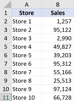
Suppose you have a data set as shown below, and you want to calculate the range for the data in column B.
Below is the formula to calculate the range for this data set:
=MAX(B2:B11)-MIN(B2:B11)
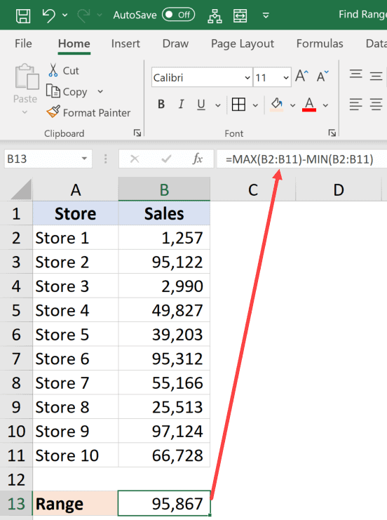
The above formula finds the maximum and the minimum value and gives us the difference.
Quite straightforward… isn’t it?
Calculate Conditional Range in Excel
In most practical cases, finding the range would not be as simple as just subtracting the minimum value from the maximum value
In real-life scenarios, you might also need to account for some conditions or outliers.
For example, you may have a data set where all the values are below 100, but there is one value that is above 500.
If you calculate arrange for this data set, it would lead to you making misleading interpretations of the data.
Thankfully, Excel has many conditional formulas that can help you sort out some of the anomalies.
Below I have a data set where I need to find the range for the sales values in column B.
If you look closely at this data, you would notice that there are two stores where the values are quite low (Store 1 and Store 3).
This could be because these are new stores or there were some external factors that impacted the sales for these specific stores.
While calculating the range for this data set, it might make sense to exclude these newer stores and only consider stores where there are substantial sales.
In this example, let’s say I want to ignore all those stores where the sales value is less than 20,000.
Below is the formula that would find the range with the condition:
=MAX(B2:B11)-MINIFS(B2:B11,B2:B11,">20000")
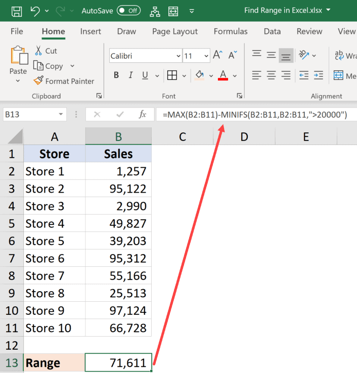
In the above formula, instead of using the MIN function, I have used the MINIFS function (it’s a new function in Excel 2019 and Microsoft 365).
This function finds the minimum value if the criteria mentioned in it are met. In the above formula, I specified the criteria to be any value that is more than 20,000.
So, the MINIFS function goes through the entire data set, but only considers those values that are more than 20,000 while calculating the minimum value.
This makes sure that values lower than 20,000 are ignored and the minimum value is always more than 20,000 (hence ignoring the outliers).
Note that the MINIFS is a new function in Excel is available only in Excel 2019 and Microsoft 365 subscription. If you’re using prior versions, you would not have this function (and can use the formula covered later in this tutorial)
If you don’t have the MINIF function in your Excel, use the below formula that uses a combination of IF function and MIN function to do the same:
=MAX(B2:B11)-MIN(IF(B2:B11>20000,B2:B11))
Just like I have used the conditional MINIFS function, you can also use the MAXIFS function if you want to avoid data points that are outliers in the other direction (i.e., a couple of large data points that can skew the data)
So, this is how you can quickly find the range in Excel using a couple of simple formulas.
I hope you found this tutorial useful.
Other Excel tutorials you may like:
- How to Calculate Standard Deviation in Excel
- How to Calculate Square Root in Excel
- How to Calculate and Format Percentages in Excel