Find a range name in excel - Word и Excel - помощь в работе с программами

So, you’ve named a range of cells, and … perhaps you forgot the location. You can find a named range by using the Go To feature—which navigates to any named range throughout the entire workbook.

You can find a named range by going to the Home tab, clicking Find & Select, and then Go To.

Or, press Ctrl+G on your keyboard.
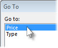
In the Go to box, double-click the named range you want to find.

Notes:

The Go to popup window shows named ranges on every worksheet in your workbook.
To go to a range of unnamed cells, press Ctrl+G, enter the range in the Reference box, and then press Enter (or click OK). The Go to box keeps track of ranges as you enter them, and you can return to any of them by double-clicking.
To go to a cell or range on another sheet, enter the following in the Reference box: the sheet name together with an exclamation point and absolute cell references. For example: sheet2!$D$12 to go to a cell, and sheet3!$C$12:$F$21 to go to range.
You can enter multiple named ranges or cell references in the Reference box. Separating each with a comma, like this: Price, Type, or B14:C22,F19:G30,H21:H29. When you press Enter or click OK, Excel will highlight all the ranges.

More about finding data in Excel

Find or replace text and numbers on a worksheet
Find merged cells
Remove or allow a circular reference
Find cells that contain formulas
Find cells that have conditional formats
Locate hidden cells on a worksheet

Need more help?

Want more options?

Explore subscription benefits, browse training courses, learn how to secure your device, and more.

Communities help you ask and answer questions, give feedback, and hear from experts with rich knowledge.

Источник

All is looking upright in Excel; you’ve been so organized, have stacked all the worksheets in the most logical order, and have obsessively named over a dozen ranges down to the T. That is what Named Ranges are for, after all, to make the usage of a cell or a range easier in your spreadsheet life.

That is just great going but how far are we falling from greatness when we can’t recall range names or their location? Uh oh. Before you write off Named Ranges as a bad idea, Excel has a few very easy-peasy ways to find Named Ranges.

By the end of this tutorial, you will learn how to find Named Ranges using the Name Manager and Paste Name feature and how to find and select a Named Range using the Find & Select feature and the Name Box.

Magnifying glasses at the ready, let’s get searching!

Method #1 – Using Find & Select Feature

Purpose: Selecting a Named Range.

Find a Named Range in Excel with the Go To command of the Find & Select feature. Find & Select is used for finding the cells containing certain data e.g., formulas, Conditional Formatting, etc. The Go To option enlists the Named Ranges in the workbook and you can select the cells of a Named Range by selecting it from the list.

The steps below demonstrate the usage of the Find & Select feature to select a Named Range in Excel:

From the Home tab, click on the Find & Select button in the Editing group and select Go To from the menu. Alternatively, use the F5 key or the keyboard shortcut Ctrl + G.

The Go To dialog box will open, listing the Named Ranges in the workbook.
Double-click on the name of the range that you want to select.
Let’s say we want to select the range named JanSales in our case example. We have named the range of the January sales figures in C6:C15 as JanSales.

Once you double-click, the Go To dialog box will close, and the Named Range will be selected on the worksheet, jumping to wherever the range is in the workbook even if it is in a different sheet.

With the help of the Go To command, we have selected the Named Range JanSales i.e. C6:C15. The name of the range is also confirmed through the Name Box.

Note: With this feature, you can only select one Named Range at a time.

Method #2 – Using Name Box

Purpose: Selecting a Named Range.

Using the Name Box you can find and select a Named Range in Excel. The Name Box is another Excel feature that shows all the Named Ranges in the file. You can find the Name Box above the worksheet area, left of the Formula Bar. Other than displaying the address of the selected cell, the Name Box is also used for creating and locating Named Ranges.

To locate a Named Range quickly with the Name Box, use these steps:

Click on the downward arrow in the Name Box to display the names in the workbook.

Select the Named Range from the drop-down menu.
Using our case example, we are going with JanSales.

When the name is clicked on, the range it corresponds to will be selected:

Method #3 – Using Name Manager

Purpose: View the location of the Named Ranges.

The Name Manager can be used to find Named Ranges in Excel. The Name Manager is a tool for handling (creating, viewing, editing, deleting, and finding) names in the spreadsheet. As the main log that holds the names in a workbook, the location of the Named Ranges is readily available in Excel’s Name Manager.

However, the Name Manager does not select a Named Range, it only displays its location. When you want to view the location of all the Named Ranges (or of any particular one) in the workbook, you can utilize the Name Manager. The steps are as follows:

Launch the Name Manager from the Formulas tab by selecting the Name Manager icon in the Defined Named Or you can use the keyboard shortcut Ctrl + F3 to do the same.

The Refers To column in the Name Manager displays the location of every Named Range in the spreadsheet.

View the location(s) as you like. Close the Name Manager after use.

Method #4 – Using Paste Name Feature

Purpose: Create a list of the location of the Named Ranges or enter values of a Named Range.

The Paste Name feature in Excel assists in finding Named Ranges. If you want the list that you just saw in the previous section extracted to somewhere in the workbook, that is a work cut out for Paste Name.

In the below-mentioned steps, you will see how to create a list of all the workbook’s Named Ranges along with their locations. There’s a little bonus trick for entering a Named Range’s value at the end of this section.

Select the cell on a worksheet where you want the list to begin.
The list will consist of 2 columns so make sure that the area you pick has the required free space for the list.

Press the F3 key to open the Paste Name dialog box.
Select the Paste List command in the dialog box.

The dialog box will close and a 2-column list of all the workbook’s names and their location will be created, starting from the selected cell.

Bonus Trick: Enter Values of Named Range

Here we have a little bonus trick using the Paste Name feature to enter the values of a Named Range. The scenario is that we know we have created a Named Range of the January sales figures but we don’t remember where in the workbook we’ve done that.

There are two less preferable methods. One is checking each tab for copy-pasting the figures. Second is locating the Named Range first before copying it. The preferable trick is to stay on the same sheet and fetch the values with a couple of steps. Those couple of steps for entering values of a Named Range using the Paste Name feature are mentioned below:

On the worksheet, select the cell that you would want the Named Range to begin from.
We’re selecting D3 as shown:

Open the Paste Name dialog box by pressing the F3
Select the Named Range that you want to enter on the worksheet.
Hit the OK

After the dialog box closes, the selected name will be first entered in D3:
Press the Enter key to enter the values of the Named Range.

The values of the selected Named Range JanSales will be entered starting from D3:

Notes:

Only the values of the Named Range will be pasted. The values will carry no format of the original Named Range.
The Named Range can be pasted from any sheet in the workbook to the active worksheet.
Only one Named Range can be pasted at a time.

Give the magnifying glass a break, today’s search ends here. We’ve covered plenty of tricks to hunt Named Ranges in Excel down. Let’s polish the magnifiers readying them and us for another Excel search. Ready? Tricky? Go!

Источник

Dim sampleRange as Range
Set sampleRange = Worksheet.Range(Cells(1,1),Cells(1,4)
sampleRange.Name = "Range1"
MsgBox sampleRange.Name

The above code will show the actual address of the range, not the name. Why?
How do I get a named range to return its name?

w5m

2,2763 gold badges33 silver badges46 bronze badges

asked Sep 2, 2010 at 19:27

For a Range, Name isn’t a string it’s a Name object, that you then take the Name property of to get the string:

MsgBox sampleRange.Name.Name

answered Sep 2, 2010 at 19:38

Lance RobertsLance Roberts

22.2k32 gold badges112 silver badges129 bronze badges

Источник

Normally, when I use the word range in my tutorials about Excel, it’s a reference to a cell or a collection of cells in the worksheet.

But this tutorial is not about that range.

A ‘Range’ is also a mathematical term that refers to the range in a data set (i.e., the range between the minimum and the maximum value in a given dataset)

In this tutorial, I will show you really simple ways to calculate the range in Excel.

What is a Range?

In a given data set, the range of that data set would be the spread of values in that data set.

To give you a simple example, if you have a data set of student scores where the minimum score is 15 and the maximum score is 98, then the spread of this data set (also called the range of this data set) would be 73

Range = 98 – 15

‘Range’ is nothing but the difference between the maximum and the minimum value of that data set.

How to Calculate Range in Excel?

If you have a list of sorted values, you just have to subtract the first value from the last value (assuming that the sorting is in the ascending order).

But in most cases, you would have a random data set where it’s not already sorted.

Finding the range in such a data set is quite straightforward as well.

Excel has the functions to find out the maximum and the minimum value from a range (the MAX and the MIN function).

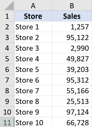
Suppose you have a data set as shown below, and you want to calculate the range for the data in column B.

Below is the formula to calculate the range for this data set:

=MAX(B2:B11)-MIN(B2:B11)

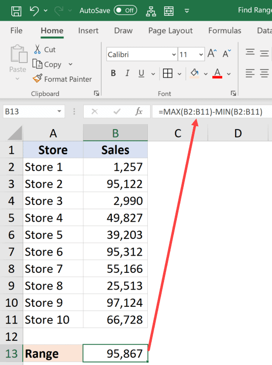
The above formula finds the maximum and the minimum value and gives us the difference.

Quite straightforward… isn’t it?

Calculate Conditional Range in Excel

In most practical cases, finding the range would not be as simple as just subtracting the minimum value from the maximum value

In real-life scenarios, you might also need to account for some conditions or outliers.

For example, you may have a data set where all the values are below 100, but there is one value that is above 500.

If you calculate arrange for this data set, it would lead to you making misleading interpretations of the data.

Thankfully, Excel has many conditional formulas that can help you sort out some of the anomalies.

Below I have a data set where I need to find the range for the sales values in column B.

If you look closely at this data, you would notice that there are two stores where the values are quite low (Store 1 and Store 3).

This could be because these are new stores or there were some external factors that impacted the sales for these specific stores.

While calculating the range for this data set, it might make sense to exclude these newer stores and only consider stores where there are substantial sales.

In this example, let’s say I want to ignore all those stores where the sales value is less than 20,000.

Below is the formula that would find the range with the condition:

=MAX(B2:B11)-MINIFS(B2:B11,B2:B11,">20000")

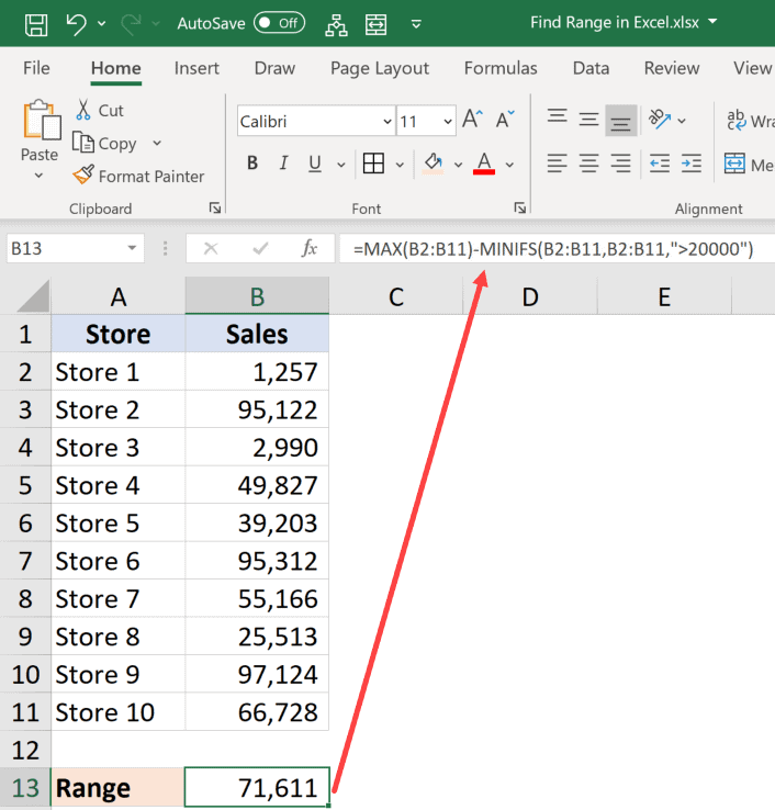
In the above formula, instead of using the MIN function, I have used the MINIFS function (it’s a new function in Excel 2019 and Microsoft 365).

This function finds the minimum value if the criteria mentioned in it are met. In the above formula, I specified the criteria to be any value that is more than 20,000.

So, the MINIFS function goes through the entire data set, but only considers those values that are more than 20,000 while calculating the minimum value.

This makes sure that values lower than 20,000 are ignored and the minimum value is always more than 20,000 (hence ignoring the outliers).

Note that the MINIFS is a new function in Excel is available only in Excel 2019 and Microsoft 365 subscription. If you’re using prior versions, you would not have this function (and can use the formula covered later in this tutorial)

If you don’t have the MINIF function in your Excel, use the below formula that uses a combination of IF function and MIN function to do the same:

=MAX(B2:B11)-MIN(IF(B2:B11>20000,B2:B11))

Just like I have used the conditional MINIFS function, you can also use the MAXIFS function if you want to avoid data points that are outliers in the other direction (i.e., a couple of large data points that can skew the data)

So, this is how you can quickly find the range in Excel using a couple of simple formulas.

I hope you found this tutorial useful.

Other Excel tutorials you may like:

How to Calculate Standard Deviation in Excel
How to Calculate Square Root in Excel
How to Calculate and Format Percentages in Excel

Источник

Naming a range of cells in Excel provide an easy way to reference those cells in a formula. If you have a workbook with a lot of data on the worksheets, naming ranges of cells can make your formulas easier to read and less confusing.

RELATED: How to Assign a Name to a Range of Cells in Excel

But if you have a particularly big spreadsheet, you may not remember which names refer to which ranges. We’ll show you how to generate a list of names and their associated cell ranges you can reference as you make formulas for that spreadsheet.

Depending on how many names you have in your workbook, you may want to use a new worksheet to store the list. Our list is not very long, but we still want to keep it separate from the rest of our data. So, right-click on the worksheet tabs at the bottom of the Excel window and select “Insert” from the popup menu. When the “Insert” dialog box displays, make sure the “General” tab is active and “Worksheet” is selected in the right box. Then, click “OK”.

Select the cell on your new worksheet where you want the list of names to start and click the Formulas tab. You can add some headings above your list if you want, like we did below.

In the Defined Names section, click “Use In Formula” and select “Paste Names” from the drop-down menu. You can also press “F3”.

NOTE: If there are no named cell ranges in your workbook, the “Use In Formula” button is not available.

On the Paste Name dialog box, all the named cell ranges display in the Paste name list. To insert the entire list into the worksheet, click “Paste List”.

The list is inserted starting in the selected cell. You might want to widen the columns so the names don’t get cut off. Simply put the cursor over the right edge of the column you want to widen until it becomes a double arrow and then double-click.

Your list of names and the corresponding cell ranges display in your worksheet. You can save your workbook like this so you have a list of your names and you can also print the worksheet if you want.

If you add names to or remove names from the workbook, delete the generated list and generate it again to obtain an updated list.