Find a number in a table in excel

We have the table in which the sales volumes of certain products are recorded in different months. It is necessary to find the data in the table, and the search criteria will be the headings of rows and columns. But the search must be performed separately by the range of the row or column. That is, only one of the criteria will be used. Therefore, you can`t apply the INDEX function here, but you need a special formula.



Finding values in the Excel table

To solve this problem, let us illustrate the example in the schematic table that corresponds to the conditions are described above.

The sheet with the table to search for values vertically and horizontally:

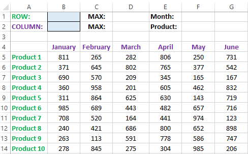
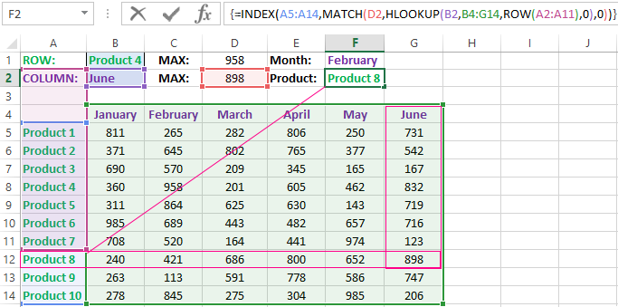
Above this table we can see the row with results. In the cell B1 we introduce the criterion for the search query, that is, the column header or the ROW name. And in the cell D1, to a search formula should return to the result of the calculation of the corresponding value. Then the second formula will work in the cell F1. She will already use the values of the cells B1 and D1 as the criteria for searching of the corresponding month.



Search of the value in the Excel ROW

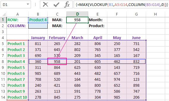
Now we are learning, in what maximum volume and in what month has been the maximum sale of the Product 4.

To search by columns:

1. In the cell B1 you need to enter the value of the Product 4 — the name of the row, that will act as the criterion.
2. In the cell D1 you need to enter the following:
3. To confirm after entering the formula, you need to press the CTRL + SHIFT + Enter hotkey combination, because she must be executed in the array. If everything is done correctly, the curly braces will appear in the formula ROW.



4. In the cell F1 you need to enter the second:
5. For confirmation, to press the key combination CTRL + SHIFT + Enter again.

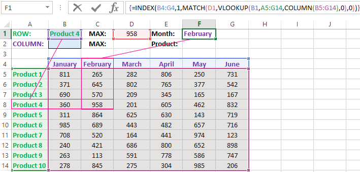
So we have found, in what month and what was the largest sale of the Product 4 for two quarters.

The principle of the formula for finding the value in the Excel ROW:

In the first argument of the VLOOKUP function (Vertical Look Up), indicates to the reference to the cell, where the search criterion is located. In the second argument indicates to the range of the cells for viewing during in the process of searching.

In the third argument of the VLOOKUP function should be indicated the number of the column from which you should to take the value against of the row named the Item 4. But since we do not previously know this number, we use the COLUMN function for creating the array of column numbers for the range B4:G15.

This allows the VLOOKUP function to collect the whole array of values. As a result, all relevant values are stored in memory for each column in the row Product 4 (namely: 360; 958; 201; 605; 462; 832). After that, the MAX function will only take the maximum number from this array and return it as the value for the cell D1, as the result of calculating.

As you can see, the construction of the formula is simple and concise. On its basis, it is possible in a similar way to find other indicators for a certain product. For example, the minimum or an average value of sales volume you need to find using for this purpose MIN or AVERAGE functions. Nothing hinders you from applying this skeleton of the formula to apply with more complex functions for implementation the most comfortable analysis of the sales report.

How can I get to the column headings from a single cell value?

For example, how effectively we displayed the month with the maximum sale, using of the second. It’s not difficult to notice that in the second formula we used the skeleton of the first formula without the MAX function. The main structure of the function is: VLOOKUP. We replaced the MAX on the MATCH, which in the first argument uses the value obtained by the previous formula. It acts as the criterion for searching for the month now.

And as a result, the MATCH function returns the column number 2, where the maximum value of the sales volume for the product is located for the product 4. After that, the INDEX function is included in the work. This function returns the value by the number of terms and column from the range specified in its arguments. Because the we have the number of column 2, and the row number in the range where the names of months are stored in any cases will be the value 1. Then we have the INDEX function to get the corresponding value from the range of B4:G4 — February (the second month).

Search the value in the Excel column

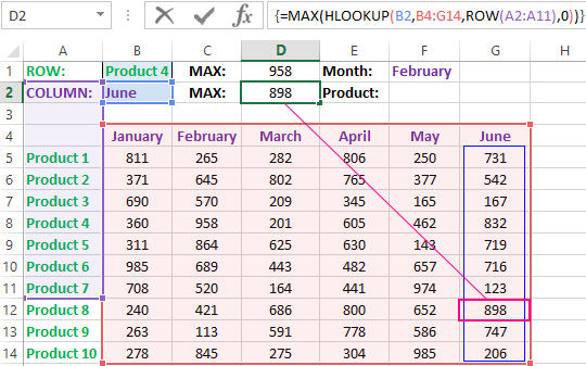
The second version of the task will be searching in the table with using the month name as the criterion. In such cases, we have to change the skeleton of our formula: the VLOOKUP function is replaced by the HLOOKUP (Horizontal Look Up) one, and the COLUMN function is replaced by the row one.

This will allow us to know what volume and what of the product the maximum sale was in a certain month.

To find what kind of the product had the maximum sales in a certain month, you should:

1. In the cell B2 to enter the name of the month June — this value will be used as the search criterion.
2. In the cell D2, you should to enter the formula:
3. To confirm after entering the formula you need to press the combination of keys CTRL + SHIFT + Enter, as this formula will be executed in the array. And the curly braces will appear in the function ROW.



4. In the cell F1, you need to enter the second:
5. You need to click CTRL + SHIFT + Enter for confirmation again.

The principle of the formula for finding the value in the Excel column

In the first argument of the HLOOKUP function, we indicate to the reference by the cell with the criterion for the search. In the second argument specifies the reference to the table argument being scanned. The third argument is generated by the ROW function, what creates in the array of ROW numbers of 10 elements in memory. So there are 10 rows in the table section.

Further the HLOOKUP function, alternately using to each number of the row, creates the array of corresponding sales values from the table for the certain month (June). Further, the MAX function is left only to select the maximum value from this array.

Then just a little modifying to the first formula by using the INDEX and MATCH functions, we created the second function to display the names of the table rows according to the cell value. The names of the corresponding rows (products) we output in F2.

ATTENTION! When using the formula skeleton for other tasks, you need always to pay attention to the second and the third argument of the search HLOOKUP function. The number of covered rows in the range is specified in the argument, must match with the number of rows in the table. And also the numbering should begin with the second ROW!

Download example search values in the columns and rows

Read also: The searching of the value in a range Excel table in columns and rows

Indeed, the content of the range generally we don’t care — we just need the row counter. That is, you need to change the arguments to: ROW(B2:B11) or ROW(C2:C11) — this does not affect in the quality of the formula. The main thing is that — there are 10 rows in these ranges, as well as in the table. And the numbering starts from the second row!

Following on from my other Microsoft Excel articles, this one is devoted to looking up information from within a range of values such as a table of data but using the functions that Excel provides.

We will look at four functions used for finding operations within Excel; VLOOKUP, HLOOKUP, MATCH and INDEX. First we will have an explanation of each and then walk through some examples of their usage. Finally in this article I will explain how to look up a value in a table based on multiple criteria using SUMPRODUCT.

Excel finding function descriptions

INDEX(array of values, row number, column number)

The INDEX function allows you to find a value within an array of values (usually a table). It takes three arguments (an argument is a value, a range or could even be another formula). The array of values (i.e. the range which can be a single row or column or have multiple rows and columns such as a table), the row and column number for which to return the intersecting value. To put it simply, specifying INDEX(my_table,3,4) will return the value of the fourth column on the third row.

You can also replace either row number of column number with a zero to specify that it should use all values of the row or column, in which case it will return an array of values rather than a single value. For example INDEX(my_table,0,4) returns all values of column 4 in my table.

MATCH(value to find, array of values, [match type])

The MATCH function finds the first occurrence of a value to find within an array of values. The function returns an error if not found or the position in the sequence of the first occurrence. The match type is optional so it can be left out or can be specified with 0, 1 or -1. Leaving it out assumes 0 as the default match type. The 0 is for an exact match but if no exact match is found you can tell Excel what do return in its place with 1 being the value nearest but below the value specified and -1 being the value higher than the one specified. However, any match type other than 0 only works when the array of values are in ascending order.

VLOOKUP(value to find, table of values, column number, [range lookup])

The VLOOKUP function stands for Vertical Lookup and searches through the rows of the first column in a table of values and returns the value from a column number specified.

The values in the first column must be in ascending order from top to bottom. If you have a table of values and you want to find a record by using the identifier in the first column and return a value from the row of date for that identifier then this is a very useful function. The range lookup is an optional setting with TRUE being a nearest match and FALSE being an exact match. FALSE will return an error if not found whereas TRUE will return the exact match if it is found but if not will still return the value in the sequence at the position before the value to find.

For example a search for “Spurs” in the following data sequence; “Queens Park Rangers”, “Southampton”, “Stoke City”, “Sunderland”, “Swansea City”, “Tottenham Hotspur” and “West Bromwich Albion” would produce “#N/A” if the range lookup was FALSE and “Southampton” if the range lookup was TRUE.

HLOOKUP(value to find, array of values, row number, [range lookup])

The HLOOKUP function stands for Horizontal Lookup and searches through the columns of the first row in an array of values and returns the value from a row number specified. The values in the first row must be in ascending order from left to right. Other than that it works and behaves in exactly the same was as a VLOOKUP.

MATCH and INDEX work fine on a range that has more than one column and row but VLOOKUP and HLOOKUP require a table with more than one column and row.

Excel finding function example workbook

The following examples look at the fixture list at the start of the English Premier League football season. I will work though a few situations where you can combine them to get the data you require.

If you want to download these examples you can do so here Fixtures.xlsx. The workbook has 3 sheets; Matches, MatchDays and Calculations.

At the beginning of the season, the fixtures are set on a week commencing basis for all 38 games and then the TV companies as well as UAFA rules come in to place and quite a few of the games are moved to alternative days. During the season, games are also postponed to other days but this workbook was put together early in August before the season started so we will just use the Match Week Number and the Date of the Commencement of fixtures for that week.

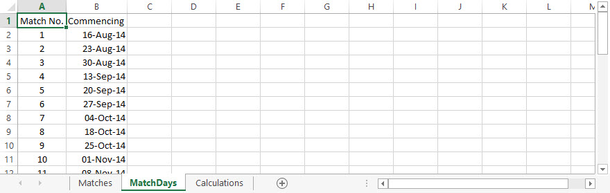
MatchDays has a simple table with two columns depicting Week Number and Date Commencing.

The Matches sheet contains a table that has its first column for the home team and first row for the away team names. So basically, using the rows and columns you can look up a home team and an away team and at their intersection find the week number when the game is due to be played. We can then look up the week commencing date on the MatchDays sheet.

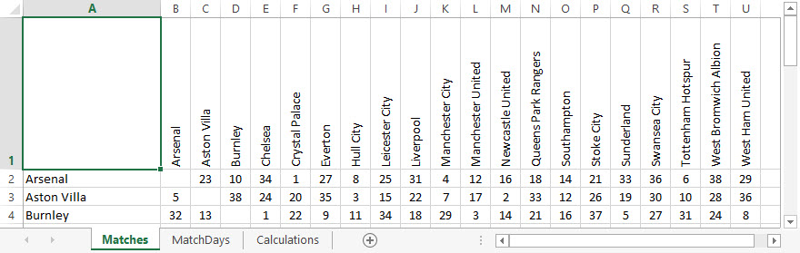
In the workbook, I’ve used some named ranges. On the MatchDays sheet the only one is Match_Days for the area of the table. On the Matches sheet, the named ranges are Matches_Matrix for the whole of the table, Match_Home_Teams for the home team column of team names and Match_Away_Teams for the away team row of team names. There are also named ranges for each home team using that teams name for some of the later examples. If you want a reminder about specifying named ranges please visit my page “Using Excel cell references and named ranges“.

Finding information examples

In the first examples, I will do something straight forward to show the functionality of the INDEX and MATCH functions.

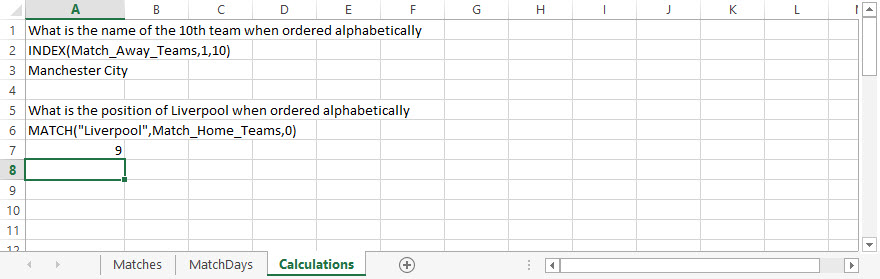
You can use the INDEX function to return a value from a list at a specified position. So if I were to ask, “What is the name of the 10th team when ordered alphabetically” I would use INDEX(Match_Away_Teams,1,10) to show that the 10th team is Manchester City.

We can also determine the position within a range of values of that a value occurs by using MATCH. So if you were to ask, “What is the position of Liverpool when the teams are ordered alphabetically” I would use MATCH(“Liverpool”,Match_Home_Teams,0) to show that the position is 9th.

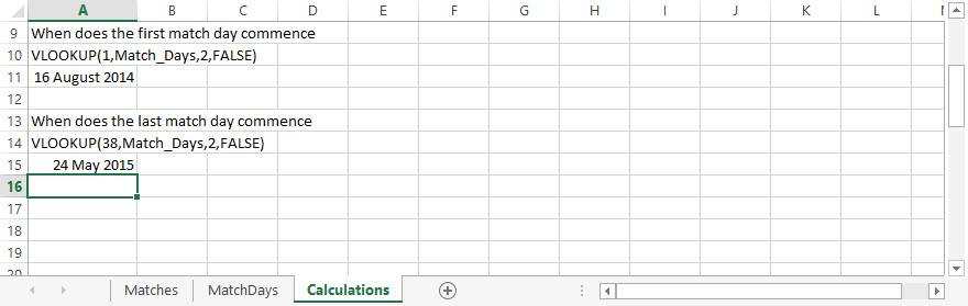
Now let us find some dates based on the MatchDays table using VLOOKUP. The table is in ascending order and I know there is a value for the commencement week for each week from 1 to 38 so I can use VLOOKUP(1,Match_Days,2,FALSE) to show the first match day (week 1) commences on the 16th August 2014 (column 2) and that the last match day (week 38) is on the 24th May 2015 using VLOOKUP(38,Match_Days,2,FALSE).

Now on to something more interesting. I’m going to use a combination of methods to look up when two teams play each other. Firstly, what week number are Everton away to Tottenham Hotspur and then what week number does the corresponding home fixture commence.

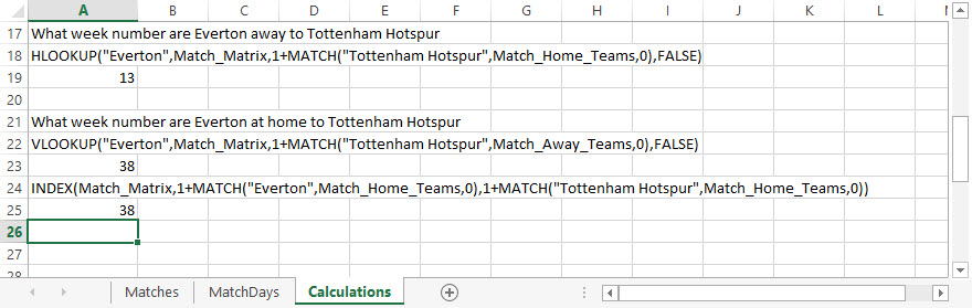
I can see that using HLOOKUP(“Everton”,Match_Matrix,1+MATCH(“Tottenham Hostpur”,Match_Home_Teams,0),FALSE) shows that Everton are away to Tottenham on the 13th week. What I am doing here is using a horizontal lookup for the column of “Everton” on the Match_Matrix table and looking up the row number using the MATCH function on the Match_Home_Team but I have to add 1 to the returned value because the Match_Matrix has both its first row and column with team names and not the matches themselves.

The corresponding fixture to find when Everton are at home to Tottenham could have been accomplished using the previous code but swapping the team names around or we can use the VLOOKUP with the same values. As a MATCH on Match_Away_Teams and Match_Home_Teams would return the same value I didn’t really need to change that in the syntax but I did do so.

There is a slightly longer way of performing the same functionality without VLOOKUP or HLOOKUP and that is using INDEX. INDEX(Match_Matrix,1+MATCH(“Everton”,Match_Home_Teams,0),1+MATCH(“Tottenham Hotspur”,Match_Home_Teams,0)) will also show that Everton are at home to Tottenham on week 38. The INDEX function uses the same table but within it you specify the row and column.

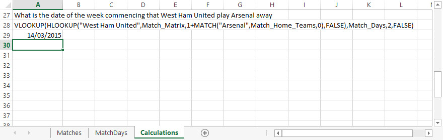
This next example gets the actual date by using a VLOOKUP on Match_Days for the week returned from a HLOOKUP of when West Ham are away to Arsenal. The result of 14 th March 2015 is given for as a result for VLOOKUP(HLOOKUP(“West Ham United”,Match_Matrix,1+MATCH(“Arsenal”,Match_Home_Teams,0),FALSE),Match_Days,2,FALSE).

Now let us say that we want to find out who a team is playing on a particular week number. For these examples I’ve simplified the code by introducing a named range for each home team’s fixture weeks. So Newcastle United have a named range of Newcastle_United.

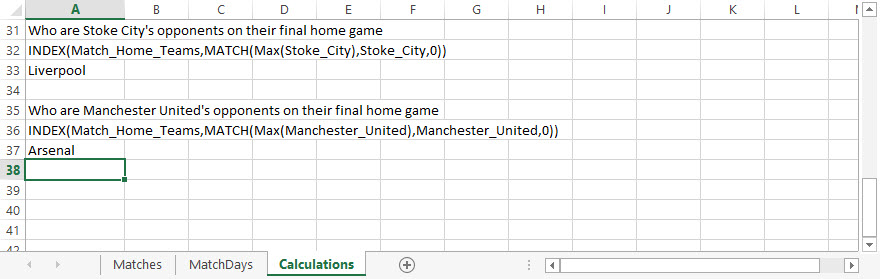
Let’s find out who Stoke City are playing on the first game of the season. This can be done using INDEX(Match_Home_Teams,MATCH(Max(Stoke_City),Stoke_City,0)) to return Liverpool as Stoke’s opponents.

I have not only introduced the additional named range for each team but I’ve also used the MAX function which takes a range of values and returns the highest regardless of the order. Basically, because a team could be home or away on the last day of the season I have used the MAX function to determine the week number of their final home game. For stoke they are at home on week 38 but in my next example, who are Manchester Unit playing on their last home match, I find that their last home game is in week 37 against Arsenal.

Using multiple criteria within Excel to find a value

We have covered the different ways to quickly find something from within something in Excel using INDEX, MATCH, VLOOKUP and HLOOKUP. All of these functions have something in common and that is they all find a single value within a table or array of values.

If you want to find values based on multiple criteria it gets a bit more complex and that job is usually undertaken by a database. However, Excel does have a function that can be used and it is called SUMPRODUCT. I had better warn you that it is not very fast when you have a lot of data but you can specify any number of criteria to look up on a table. You can download the following example here sumproduct.xlsx.

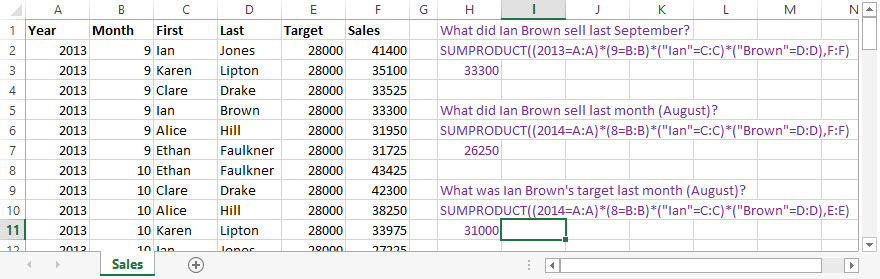
In this example, I’ve set up a table for sales and it does not need to be in any particular order as SUMPRODUCT will search through until it finds a match for the criteria you specify. The syntax to use is SUMPRODUCT(criteria, array of results). So for my example, let’s say I want to find what Ian Brown’s sales were in August 2014. I would write SUMPRODUCT((2014=A:A)*(8=B:B)*(“Ian”=C:C)*(“Brown”=D:D),F:F). Each of the criteria you specify you wrap in parentheses and use the multiplication operator to join them. I haven’t named any ranges here but you can see that I am saying column A must have 2014 in it, column B must have an 8 in it, column C must have the value “Ian” and column D must equal “Brown”. The final part is what to return and I want the corresponding value from the Sales column, which is column F.

That’s it for finding values using functions in Excel and I hope you found these examples useful.

In this example, the goal is to test the passwords in column B to see if they contain a number. This is a surprisingly tricky problem because Excel doesn’t have a function that will let you test for a number inside a text string directly. Note this is different from checking if a cell value is a number. You can easily perform that test with the ISNUMBER function. In this case, however, we to test if a cell value contains a number, which may occur anywhere. One solution is to use the FIND function with an array constant. In Excel 365, which supports dynamic array formulas, you can use a different formula based on the SEQUENCE function. Both approaches are explained below.

FIND function

The FIND function is designed to look inside a text string for a specific substring. If FIND finds the substring, it returns a position of the substring in the text as a number. If the substring is not found, FIND returns a #VALUE error. For example:

=FIND("p","apple") // returns 2
=FIND("z","apple") // returns #VALUE!

We can use this same idea to check for numbers as well:

=FIND(3,"app637") // returns 5
=FIND(9,"app637") // returns #VALUE!

The challenge in this case is that we need to check the values in column B for ten different numbers, 0-9. One way to do that is to supply these numbers as the array constant {0,1,2,3,4,5,6,7,8,9}. This is the approach taken in the formula in cell D5:

=COUNT(FIND({0,1,2,3,4,5,6,7,8,9},B5))>0

Inside the COUNT function, the FIND function is configured to look for all ten numbers in cell B5:

FIND({0,1,2,3,4,5,6,7,8,9},B5)

Because we are giving FIND ten values to look for, it returns an array with 10 results. In other words, FIND checks the text in B5 for each number and returns all results at once:

{#VALUE!,4,5,6,#VALUE!,#VALUE!,#VALUE!,#VALUE!,#VALUE!,#VALUE!}

Unless you look at arrays often, this may look pretty cryptic. Here is the translation: The number 1 was found at position 4, the number 2 was found at position 5, and the number 3 was found at position 6. All other numbers were not found and returned #VALUE errors. 

We are very close now to a final formula. We simply need to tally up results. To do this, we nest the FIND formula above inside the COUNT function like this:

=COUNT(FIND({0,1,2,3,4,5,6,7,8,9},B5))

FIND returns the array of results directly to COUNT, which counts the numbers in the array. COUNT only counts numeric values, and ignores errors. This means COUNT will return a number greater than zero if there are any numbers in the value being tested. In the case of cell B5, COUNT returns 3.

The last step is to check the result from COUNT and force a TRUE or FALSE result. We do this by adding «>0» to the end of formula:

=COUNT(FIND({0,1,2,3,4,5,6,7,8,9},B5))>0

Now the formula will return TRUE or FALSE. To display a custom result, you can use the IF function:

=IF(COUNT(FIND({0,1,2,3,4,5,6,7,8,9},B5))>0, "Yes", "No")

The original formula is now nested inside IF as the logical_test argument. This formula will return «Yes» if B5 contains a number and «No» if not.

SEQUENCE function

In Excel 365, which offers dynamic array formulas, we can take a different approach to this problem.

=COUNT(--MID(B5,SEQUENCE(LEN(B5)),1))>0

This isn’t necessarily a better approach, just a different way to solve the same problem. At the core, this formula uses the MID function together with the SEQUENCE function to split the text in cell B5 into an array:

MID(B5,SEQUENCE(LEN(B5)),1)

Working from the inside out, the LEN function returns the length of the text in cell B5:

LEN(B5) // returns 6

This number is returned to the SEQUENCE function as the rows argument, and SEQUENCE returns an array of numbers, 1-6:

=SEQUENCE(LEN(B5))
=SEQUENCE(6)
={1;2;3;4;5;6}

This array is returned to the MID function as the start_num argument, and, with num_chars set to 1, the MID function returns an array that contains the characters in cell B5:

=MID(B5,{1;2;3;4;5;6},1)
={"a";"b";"c";"1";"2";"3"}

We can now simplify the original formula to:

=COUNT(--{"a";"b";"c";"1";"2";"3"})>0

We use the double-negative (—) to get Excel to try and coerce the values in the array into numbers. The result looks like this:

=COUNT({#VALUE!;#VALUE!;#VALUE!;1;2;3})>0

The math operation created by the double negative (—) returns an actual number when successful and a #VALUE! error when the operation fails. The COUNT function counts the numbers, ignoring any errors, and returns 3. As above, we check the final count with «>0», and the result for cell B5 is TRUE.

Note: as you might guess, you can easily adapt this formula to count numbers in a text string.

Cell equals number?

Note that the formulas above are too complex if you only want to test if a cell equals a number. In that case, you can simply use the ISNUMBER function like this:

=ISNUMBER(A1)