
PivotTables are great for taking large datasets and creating in-depth detail summaries.

You can insert one or more slicers for a quick and effective way to filter your data. Slicers have buttons you can click to filter the data, and they stay visible with your data, so you always know what fields are shown or hidden in the filtered PivotTable.
-
Select any cell within the PivotTable, then go to Pivot Table Analyze > Insert Slicer
 .
. -
Select the fields you want to create slicers for. Then select OK.
-
Excel will place one slicer on the worksheet for each selection you made, but it’s up to you to arrange and size them however is best for you.
-
Click the slicer buttons to select the items you want to show in the PivotTable.
 .
.
Manual filters use AutoFilter. They work in conjunction with slicers, so you can use a slicer to create a high-level filter, then use AutoFilter to dive deeper.
-
To display AutoFilter, select the Filter drop-down arrow
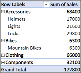
, which varies depending on the report layout.Compact Layout
The Value field is in the Rows area
The Value field is in the Columns area
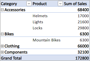
Outline/Tabular Layout
Displays the Values field name in the top left corner
-
To filter by creating a conditional expression, select Label Filters, and then create a label filter.
-
To filter by values, select Values Filters and then create a values filter.
-
To filter by specific row labels (in Compact Layout) or column labels (in Outline or Tabular Layout), uncheck Select All, and then select the check boxes next to the items you want to show. You can also filter by entering text in the Search box.
-
Select OK.
 , which varies depending on the report layout.
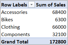
Tip: You can also add filters to the PivotTable’s Filter field. This also gives you the ability to create individual PivotTable worksheets for each item in the Filter field. For more information, see Use the Field List to arrange fields in a PivotTable.
You can also apply filters to show the top or bottom 10 values or data that meets the certain conditions.
-
To display AutoFilter, select the Filter drop-down arrow
, which varies depending on the report layout.Compact Layout
The Value field is in the Rows area
The Value field is in the Columns area
Outline/Tabular Layout
Displays the Values field name in the top left corner
-
Select Values Filters > Top 10.
-
In the first box, select Top or Bottom.
-
In the second box, enter a number.
-
In the third box, do the following:
-
To filter by number of items, pick Items.
-
To filter by percentage, pick Percentage.
-
To filter by sum, pick Sum.
-
-
In the fourth box, select a Values field.
By using a report filter, you can quickly display a different set of values in the PivotTable. Items you select in the filter are displayed in the PivotTable, and items that are not selected will be hidden. If you want to display filter pages (the set of values that match the selected report filter items) on separate worksheets, you can specify that option.
Add a report filter
-
Click anywhere inside the PivotTable.
The PivotTable Fields pane appears.
-
In the PivotTable Field List, click on the field in an area and select Move to Report Filter.
You can repeat this step to create more than one report filter. Report filters are displayed above the PivotTable for easy access.
-
To change the order of the fields, in the Filters area, you can either drag the fields to the position that you want, or double-click on a field and select Move Up or Move Down. The order of the report filters will be reflected accordingly in the PivotTable.
Display report filters in rows or columns
-
Click the PivotTable or the associated PivotTable of a PivotChart.
-
Right-click anywhere in the PivotTable, and then click PivotTable Options.
-
In the Layout tab, specify these options:
-
In Report Filter area, in the Arrange fields list box, do one of the following:
-
To display report filters in rows from top to bottom, select Down, Then Over.
-
To display report filters in columns from left to right, select Over, Then Down.
-
-
In the Filter fields per column box, type or select the number of fields to display before taking up another column or row (based on the setting of Arrange fields you specified in the previous step).
-
Select items in the report filter
-
In the PivotTable, click the dropdown arrow next to the report filter.
-
Select the checkboxes next to the items that you want to display in the report. To select all items, click the checkbox next to (Select All).
The report filter now displays the filtered items.
Display report filter pages on separate worksheets
-
Click anywhere in the PivotTable (or the associated PivotTable of a PivotChart ) that has one or more report filters.
-
Click PivotTable Analyze (on the ribbon) > Options > Show Report Filter Pages.
-
In the Show Report Filter Pages dialog box, select a report filter field, and then click OK.
-
In the PivotTable, select one or more items in the field that you want to filter by selection.
-
Right-click an item in the selection, and then click Filter.
-
Do one of the following:
-
To display the selected items, click Keep Only Selected Items.
-
To hide the selected items, click Hide Selected Items.
Tip: You can display hidden items again by removing the filter. Right-click another item in the same field, click Filter, and then click Clear Filter.
-
If you want to apply multiple filters per field, or if you don’t want to show Filter buttons in your PivotTable, here’s how you can turn these and other filtering options on or off:
-
Click anywhere in the PivotTable to show the PivotTable tabs on the ribbon.
-
On the PivotTable Analyze tab, click Options.
-
In the PivotTable Options dialog box, click the Totals & Filters tab.
-
In the Filters area, check or uncheck the Allow multiple filters per field box depending on what you need.
-
Click the Display tab, and then check or uncheck the Display Field captions and filters check box, to show or hide field captions and filter drop downs.
-
You can view and interact with PivotTables in Excel for the web by creating slicers and by manual filtering.
Slicers provide buttons that you can click to filter tables, or PivotTables. In addition to quick filtering, slicers also indicate the current filtering state, which makes it easy to understand what exactly is currently displayed.

For more information, see Use slicers to filter data.
If you have the Excel desktop application, you can use the Open in Excel button to open the workbook and create new slicers for your PivotTable data there. Click Open in Excel and filter your data in the PivotTable.
Manual filters use AutoFilter. They work in conjunction with slicers, so you can use a slicer to create a high-level filter, then use AutoFilter to dive deeper.
-
To display AutoFilter, select the Filter drop-down arrow
, which varies depending on the report layout.Single Column
The default Layout displays the Value field in the Rows areaSeparate Column
Displays the nested Row field in a distinct column -
To filter by creating a conditional expression, select <Field name> > Label Filters, and then create a label filter.
-
To filter by values, select <Field name> > Values Filters and then create a values filter.
-
To filter by specific row labels, select Filter, uncheck Select All, and then select the check boxes next to the items you want to show. You can also filter by entering text in the Search box.
-
Select OK.
Tip: You can also add filters to the PivotTable’s Filter field. This also gives you the ability to create individual PivotTable worksheets for each item in the Filter field. For more information, see Use the Field List to arrange fields in a PivotTable.
-
Click anywhere in the PivotTable to show the PivotTable tabs (PivotTable Analyze and Design) on the ribbon.
-
Click PivotTable Analyze > Insert Slicer.
-
In the Insert Slicers dialog box, check the boxes of the fields you want to create slicers for.
-
Click OK.
A slicer appears for each field you checked in the Insert Slicers dialog box.
-
In each slicer, click the items you want to show in the PivotTable.
Tip: To change how the slicer looks, click the slicer to show the Slicer tab on the ribbon. You can apply a slicer style or change settings using the various tab options.
-
In the PivotTable, click the arrow
on Row Labels or Column Labels. -
In the list of row or column labels, uncheck the (Select All) box at the top of the list, and then check the boxes of the items you want to show in your PivotTable.
-
The filtering arrow changes to this icon
to indicate that a filter is applied. Click it to change or clear the filter by clicking Clear Filter From <Field Name>.To remove all filtering at once, click PivotTable Analyze tab > Clear > Clear Filters.
 to indicate that a filter is applied. Click it to change or clear the filter by clicking Clear Filter From <Field Name>.
By using a report filter, you can quickly display a different set of values in the PivotTable. Items you select in the filter are displayed in the PivotTable, and items that are not selected will be hidden. If you want to display filter pages (the set of values that match the selected report filter items) on separate worksheets, you can specify that option.
Add a report filter
-
Click anywhere inside the PivotTable.
The PivotTable Fields pane appears.
-
In the PivotTable Field List, click on the field in an area and select Move to Report Filter.
You can repeat this step to create more than one report filter. Report filters are displayed above the PivotTable for easy access.
-
To change the order of the fields, in the Filters area, you can either drag the fields to the position that you want, or double-click on a field and select Move Up or Move Down. The order of the report filters will be reflected accordingly in the PivotTable.
Display report filters in rows or columns
-
Click the PivotTable or the associated PivotTable of a PivotChart.
-
Right-click anywhere in the PivotTable, and then click PivotTable Options.
-
In the Layout tab, specify these options:
-
In Report Filter area, in the Arrange fields list box, do one of the following:
-
To display report filters in rows from top to bottom, select Down, Then Over.
-
To display report filters in columns from left to right, select Over, Then Down.
-
-
In the Filter fields per column box, type or select the number of fields to display before taking up another column or row (based on the setting of Arrange fields you specified in the previous step).
-
Select items in the report filter
-
In the PivotTable, click the dropdown arrow next to the report filter.
-
Select the checkboxes next to the items that you want to display in the report. To select all items, click the checkbox next to (Select All).
The report filter now displays the filtered items.
Display report filter pages on separate worksheets
-
Click anywhere in the PivotTable (or the associated PivotTable of a PivotChart ) that has one or more report filters.
-
Click PivotTable Analyze (on the ribbon) > Options > Show Report Filter Pages.
-
In the Show Report Filter Pages dialog box, select a report filter field, and then click OK.
You can also apply filters to show the top or bottom 10 values or data that meets the certain conditions.
-
In the PivotTable, click the arrow
next to Row Labels or Column Labels. -
Right-click an item in the selection, and then click Filter > Top 10 or Bottom 10.
-
In the first box, enter a number.
-
In the second box, pick the option you want to filter by. The following options are available:
-
To filter by number of items, pick Items.
-
To filter by percentage, pick Percentage.
-
To filter by sum, pick Sum.
-
-
In the search box, you can optionally search for a particular value.
-
In the PivotTable, select one or more items in the field that you want to filter by selection.
-
Right-click an item in the selection, and then click Filter.
-
Do one of the following:
-
To display the selected items, click Keep Only Selected Items.
-
To hide the selected items, click Hide Selected Items.
Tip: You can display hidden items again by removing the filter. Right-click another item in the same field, click Filter, and then click Clear Filter.
-
If you want to apply multiple filters per field, or if you don’t want to show Filter buttons in your PivotTable, here’s how you can turn these and other filtering options on or off:
-
Click anywhere in the PivotTable to show the PivotTable tabs on the ribbon.
-
On the PivotTable Analyze tab, click Options.
-
In the PivotTable Options dialog box, click the Layout tab.
-
In the Layout area, check or uncheck the Allow multiple filters per field box depending on what you need.
-
Click the Display tab, and then check or uncheck the Field captions and filters check box, to show or hide field captions and filter drop downs.
-
Need more help?
You can always ask an expert in the Excel Tech Community or get support in the Answers community.
See Also
Video: Filter data in a PivotTable
Create a PivotTable to analyze worksheet data
Create a PivotTable to analyze external data
Create a PivotTable to analyze data in multiple tables
Sort data in a PivotTable
Group or ungroup data in a PivotTable
There are different ways you can filter data in a Pivot Table in Excel.
As you’ll go through this tutorial, you’ll see there are different data filter options available based on the data type.
Types of Filters in a Pivot Table
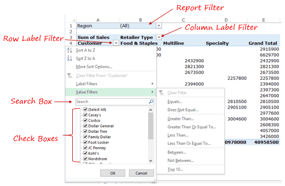
Here is a demo of the types of filters available in a Pivot Table.
Let’s look at these filters one by one:
- Report Filter: This filter allows you to drill down into a subset of the overall dataset. For example, if you have retail sales data, you can analyze data for each region by selecting one or more than regions (yes, it allows multiple selections as well). You create this filter by dragging and dropping the Pivot Table field into the Filters area.
- Row/Column Label Filter: These filters allow you to filter relevant data based on the field items (such as filter specific item or item that contains a specific text) or the values (such as filter top 10 items by value or items with a value greater than/less than a specified value).
- Search Box: You can access this filter within the row/column label filter and this allows you to quickly filter based on the text you enter. For example, if you want data for Costco only, just type Costco here and it will filter that for you.
- Check Boxes: These allow you to select specific items from a list. For example, if you want to hand pick retailers to analyze, you can do this here. Alternatively, you can also selectively exclude some retailers by unchecking it.
Note, there are two more filtering tools available to a user: Slicers and Timelines (which are not covered in this tutorial).
Let’s see some practical examples of how to use these to filter data in a Pivot Table.
Examples of Using Filters in Pivot Table
The following examples are covered in this section:
- Filter Top 10 Items by Value/Percent/Sum.
- Filter Items based on Value.
- Filter Using Label Filter.
- Filter Using Search Box.
Filter Top 10 Items in a Pivot Table
You can use the top 10 filter option in a Pivot Table to:
- Filter top/bottom items by value.
- Filter top/bottom items that make up a Specified Percent of the Values.
- Filter top/bottom Items that make up a Specified Value.
Suppose you have a Pivot Table as shown below:

Let’s see how to use the Top 10 filter with this data set.
Filter Top/Bottom Items by Value
You can use the Top 10 filter to get a list of top 10 retailers based on the sales value.
Here are the steps to do this:
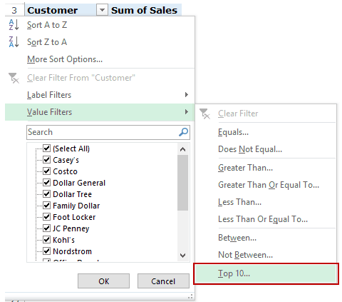
- Go to Row Label filter –> Value Filters –> Top 10.

- In the Top 10 Filter dialog box, there are four options that you need to specify:
This will give you a filtered list of 10 retailers based on their sales value.

You can use the same process to get the bottom 10 (or any other number) items by value.
Filter Top/Bottom Items that make up a Specified Percent of the Value
You can use the top 10 filter to get a list of top 10 percent (or any other number, say 20 percent, 50 percent, etc.) of items by value.
Let’s say you want to get the list of retailers that make up 25% of the total sales.
Here are the steps to do this:
- Go to Row Label filter –> Value Filters –> Top 10.
- In the Top 10 Filter dialog box, there are four options that you need to specify:
This will give you a filtered list of retailers that make up 25% of the total sales.

You can use the same process to get the retailers that make up the bottom 25% (or any other percentage) of the total sales.
Filter Top/Bottom Items that make up a Specified Value
Let’s say you want to find out the top retailers that account for 20 million in sales.
You can do this using the Top 10 filter in the Pivot Table.
To do this:
- Go to Row Label filter –> Value Filters –> Top 10.
- In the Top 10 Filter dialog box, there are four options that you need to specify:
This will give you a filtered list of top retailers that make up 20 Million of the total sales.

Filter Items based on Value
You can filter items based on the values in the columns in the values area.
Suppose you have a pivot table created using retail sales data as shown below:
You can filter this list based on the sales value. For example, suppose you want to get a list of all the retailers that have sales more than 3 million.
Here are the steps to do this:
- Go to Row Label filter –> Value Filters –> Greater Than.

- In the Value Filter dialog box:
- Click OK.

This would instantly filter the list and show only those retailers that have sales more than 3 million.

Similarly, there are many other conditions that you can use such as equal to, does not equal to, less than, between, etc.

Filter Data Using Label Filters
Label filters come in handy when you have a huge list and you want to filter specific items based on its name/text.
For example, in the list of retailers, I can quickly filter all the dollar stores by using the condition ‘dollar’ in the name.
Here are the steps to do this:
- Go to Row Label filter –> Label Filters –> Contains.

- In the label filter dialog box:
- Click OK.

You can also use wildcard characters along with the text.
Note that these filters are not additive. So if you search for the term ‘Dollar’, it will give you a list of all the stores that have the word ‘dollar’ in it, but if you then again use this filter to get a list using another term, it will filter based on the new term.
Similarly, you can use other label filters such as begins with, ends with does not contain, etc.
Filter Data Using Search Box
Filtering a list using search box is a lot like the contains option in the label filter.
For example, if you have to filter all the retailers that have the name ‘dollar’ in it, simply type dollar in the search box and it will filter the results.
Here are the steps:
This would instantly filter all the retailers that contain the term ‘dollar’.

You can use wildcard characters in the search box. For example, if you want to get the name of all the retailers that start with the alphabet T, use the search string as T* (T followed by an asterisk). Since asterisk represents any number of characters, this means that the name can contain any number of characters after T.

Similarly, if you want to get the list of all the retailers that end with the alphabet T, use the search term as *T (asterisk followed by T).
There are a few important things to know about the search bar:
- If you filter once with one criterion and then filter again with another, the first criterion is discarded and you get a list of the second criteria. The filtering is not additive.
- A benefit of using search box is that you can manually deselect some of the results. For example, if you have a huge list of financial companies and you only want to filter banks, you can search for the term ‘bank’. But in case some companies creep in that are not banks, you can simply uncheck it and keep it out.
- You can not exclude specific results. For example, if you want to exclude only the retailers that contain dollar in it, there is no way to do this using the search box. This can, however, be done using the label filter using the ‘does not contain’ condition.
You May Also Like the Following Pivot Table Tutorials:
- Creating a Pivot Table in Excel – A Step by Step Tutorial.
- Preparing Source Data For Pivot Table.
- Group Numbers in Pivot Table in Excel.
- Group Dates in Pivot Tables in Excel.
- Refresh Pivot Table in Excel.
- Delete a Pivot Table in Excel.
- How to Add and Use an Excel Pivot Table Calculated Field.
- Apply Conditional Formatting in a Pivot Table in Excel.
- Pivot Cache in Excel – What Is It and How to Best Use It?
- Replace Blank Cells with Zeros in Excel Pivot Tables.
- Count Distinct Values in Pivot Table
Filters in PivotTables are not similar to filters in the tables or data we use. In PivotTable filters, we have two methods to use. One is by right-clicking on the PivotTable, and we will find the “Filter” option for the PivotTable filter. Another way is using the filter options provided in the PivotTable fields.
How to Filter in a Pivot Table?
The PivotTable is an Excel spreadsheet tool that allows us to summarize, group, and perform mathematical operations like SUM, AVERAGE, COUNT, etc., from the organized data stored in a database. Apart from the mathematical operations, the PivotTable has one of the best features: filtering, which allows us to extract defined results from our data.
Let us look at multiple ways of using a filter in an Excel Pivot table: –
Table of contents
- How to Filter in a Pivot Table?
- #1 – Inbuilt filter in the Excel Pivot Table
- #2 – Create a filter to Values Area of an Excel Pivot table
- #3 – Display a list of multiple items in a Pivot Table Filter.
- Using Slicers
- Create List of cells with Pivot Table Filter Criteria: –
- List of Comma Separated Values in Excel Pivot Table Filter: –
- Things to remember about Excel Pivot Table Filter
- Recommended Articles
#1 – Inbuilt filter in the Excel Pivot Table
- Let us have the data in one of the worksheets.
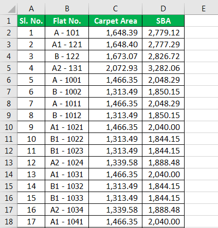
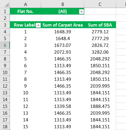
The above data consists of 4 columns: Sr.No, Flat No., Carpet Area, and SBA.
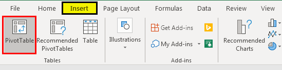
- Go to the “Insert” tab and select a PivotTable, as shown below.
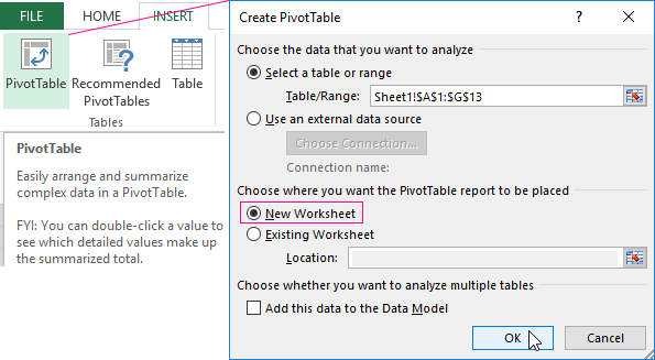
- The “Create a PivotTable” window pops out when you click on the PivotTable.
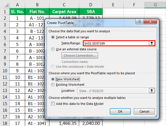
In this window, we can select a table or a range to create a PivotTable. Else, we can also use an external data source.
We can also place the PivotTable report in the same worksheet or a new one. For example, we can see this in the above picture.
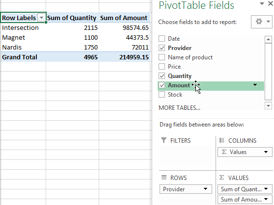
- The “PivotTable Fields” is available on the right end of the sheet as below.
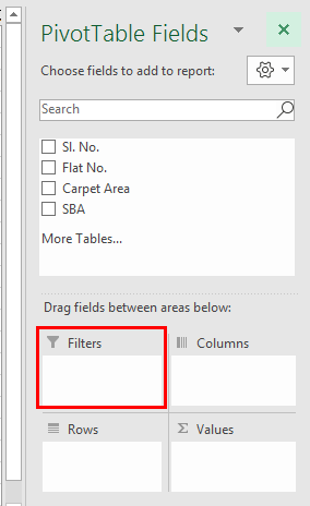
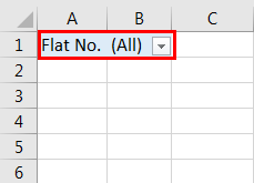
- We can observe the filter field, where we can drag the fields into filters to create a PivotTable filter. Let us drag the “Flat.No” field into “Filters.” We can see the filter for flat no’s would have been created.
- From this, we can filter the flat numbers as per our requirement, which is the normal way of creating the filter in the PivotTable.
#2 – Create a filter for the Values Area of an Excel Pivot table
Generally, when we take data into value areas, we would not create any filter for those Pivot Table fieldsPivot table calculated fields are formulas with reference to other fields, and calculated values refer to other values within a specific pivot field.read more. However, we can see it below.
We can observe that there is no filter option for value areas: Sum of SBA and Sum of Carpet Area. But we can create it, which helps us in various decision-making purposes.
- Firstly, we must select any cell next to the table and click on the “Filter” in the “Data” tab.
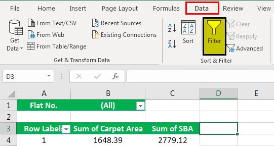
- We can see the filter gets in the “Values” area.
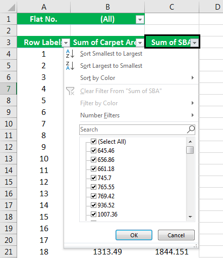
As we got the filters, we can perform different types of operations from value areas, like sorting them from largest to smallest to know top sales/area/anything. Similarly, we can sort from smallest to largest, sorting by color, and even perform number filters like <=,<,>=,>, and many more. So, it plays a major role in decision-making in any organization.
#3 – Display a list of multiple items in a Pivot Table Filter.
The above example taught us about creating a filter in the PivotTable.
Now, let us look at how we display the list differently.
The three most important ways of displaying a list of multiple items in a PivotTable filter are:
- Using Slicers.
- Creating a list of cells with filter criteria.
- List of comma-separated-values.
Using Slicers
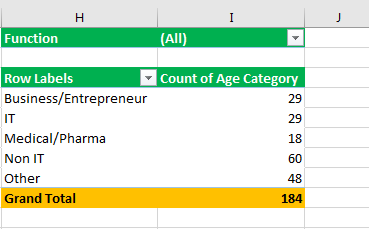
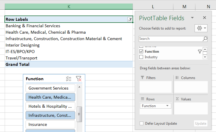
- Let us have a simple PivotTable with columns: Region, Month, Unit no, Function, Industry, Age Category.
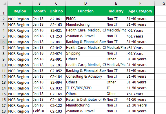
- First, create a PivotTable using the above-given data. Then, select the data, go to the “Insert” tab, select a “PivotTable” option, and create a PivotTable.
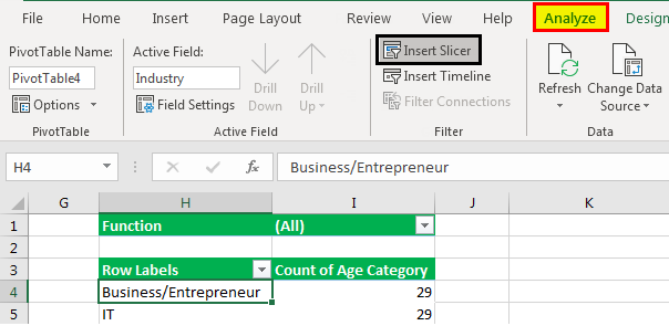
- From this example, we will consider the function of our filter. First, let us check how it can be listed using slicers and varies as per our selection. It is simple: we select any cell inside the PivotTable, go to the “Analyze” tab on the ribbon, and choose the “Insert Slicer.”
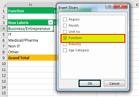
- Then, we need to insert the slide in the slicer of the field in our filter area. So, in this case, we must select the “Function” field in our filter area and then press the “OK” button, which will add a slicer to the sheet.
- We can see items highlighted in the slicer are those highlighted in our PivotTable filter criteria in the filter drop-down menu.
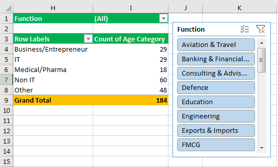
Now, this is a pretty simple solution that does display the filter criteria. By this, we can easily filter out multiple items and can see the result varying in value areas. From the below example, it is clear that we had selected the functions that are visible in the slicer and can find out the count of age category for different industries (which are row labels that we had dragged into the row label field), which are associated with those functions that are in a slicer. We can change the function per our requirement and observe that the results vary as per the selected items.
However, suppose you have many items on your list here, which is long. In that case, we might not display those items properly. You might have to scroll to see which items are selected, leading us to the next solution: list the filter criteria in cells.
So, “Create List of Cells With Pivot Table Filter Criteria” comes to our rescue.
Create a List of cells with Pivot Table Filter Criteria: –
We will use a connected PivotTable and the above slicer here to connect two PivotTables.
- Let us create a duplicate copy of the existing PivotTable and paste it into a blank cell.
So, we have a duplicate copy of our PivotTable, and we will modify it slightly to show the “Function” field in the “Rows” area.
To do this, we have to select any cell inside our PivotTable here, go over to the PivotTable field list, and remove industry from the “Rows.” Also, removing the “Count of Age” category from the “Values” area, we will take the “Function” that is in our “Filters” area to the “Rows” area. So, now we can see that we have a list of our filter criteria. If we look over here in our filter drop-down menu, we have the list of items in slicers and function filters.
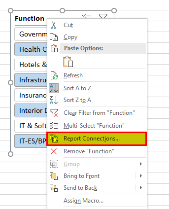
- Now, we have a list of our PivotTable filter criteria. It works because both of these PivotTables are connected by the slicer. We can right-click anywhere on the slicer to report connections.
- PivotTable connections will open up a menu showing that these PivotTables are connected as checkboxes are checked.
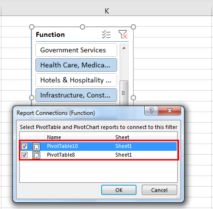
It means whenever one change is made in the first PivotTable, it automatically gets reflected in the other.
We can move PivotTables anywhere. For example, we can use it in any financial model and change row labels.
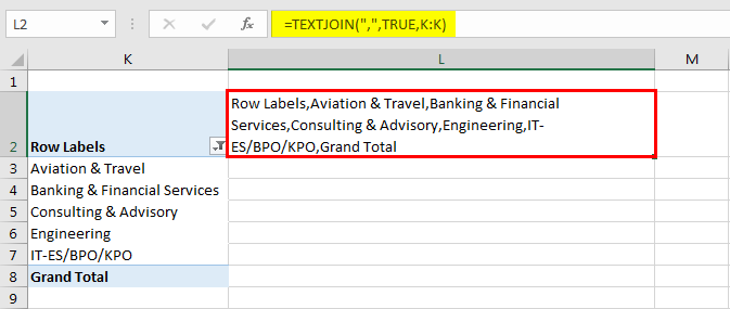
List of Comma Separated Values in Excel Pivot Table Filter: –
So, the third way to display our PivotTable filter criteria is in a single cell with a list of comma-separated values. We can do that with the TEXTJOIN function. We still need the tables we used earlier and just used a formula to create this string of values and separate them with commas.
It is a new formula or function introduced in Excel 2016, called TEXTJOIN(If there is no 2016, you can also use the CONCATENATE function); text joining makes this process much easier.
The TEXTJOIN function provides us with three different arguments:
- Delimiter – It can be a comma or space.
- Ignore empty – TRUE or FALSE to ignore blank cells or not.
- Text – Add or specify a range of cells that contain the values we want to concatenate.
Let us type the TEXTJOIN – (delimiter- which would be “,” in this case, TRUE (as we should ignore empty cells), K: K(like the list of selected items from the filter will be available in this column)to join any value and also ignore any empty value).
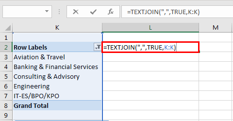
- Now, we see getting a list of all our PivotTable filter criteria joined by a string. So it is a comma-separated list of values.
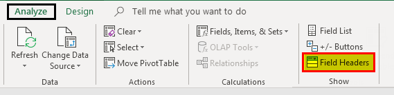
- We could hide the cell if we did not want to show these filter criteria in the formula. Select the cell and go to the “Analyze” options tab. Click on “Field Headers,” and that will hide the cell.
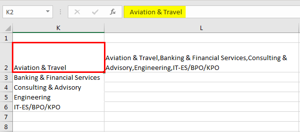
So, now we have the list of values in their PivotTable filter criteria. If we change the PivotTable filter, it reflects in all the methods. We can use any one of them. But eventually, for a comma-separated solution, a slicer and the list are required. We can hide them if we do not want to display the tables.
Things to remember about Excel Pivot Table Filter
- The PivotTable filtering is not an additive because when we select one criterion and want to filter again with other criteria, the first one will get discarded.
- We got a special feature in the PivotTable filter: “Search Box,” which allows us to manually deselect some of the results we do not want. E.g., If we have a huge list and there are blanks too, then to select blank, we can easily choose by searching for blanks in the search box rather than scrolling down till the end.
- We cannot exclude certain results with a condition in the PivotTable filter, but we can do it by using the “Label Filter.” E.g., If we want to select any product with a certain currency like rupee or dollar, etc., then we can use a label filter – ‘does not contain’ and should give the condition.
You can download this Excel Pivot table filter template from here – Pivot Table Filter Excel Template.
Recommended Articles
This article is a guide to the PivotTable Filter in Excel. Here, we discuss how to filter data in a PivotTable with the help of examples and a downloadable Excel template. You may learn more about Excel from the following articles: –
- Excel Pivot Table From Multiple SheetsPivot Table is a basic data analysis tool that calculates, summarizes, & analyses the data of a more extensive table. To create a Pivot Table from Multiple Sheets, you can use a few shortcuts & features as per the specified conditions. read more
- Pivot Table Count Unique
- How to Delete the Pivot Table?To delete a pivot table in Excel, you must first select it. Then go to the Analyze menu tab under the Design and Analyze menu tabs and select actions. Then, from the Select option’s drop-down option, select Entire Pivot Table to delete it.read more
- Pivot Chart in ExcelIn Excel, a pivot chart is a built-in feature that allows you to summarize selected rows and columns of data in a spreadsheet. It is a visual representation of a pivot table that helps in the summarization and analysis of datasets, patterns, and trends.read more
See all How-To Articles
This tutorial demonstrates how to filter pivot table values in Excel and Google Sheets.
Built-in Pivot Table Filter
When you create a pivot table, the column headers from the data become fields for the pivot table. Filtering in a pivot table is similar to applying any other filter in Excel.
- In the PivotTable Fields window, drag fields down to one of four areas to build the table. One area is for Filters.
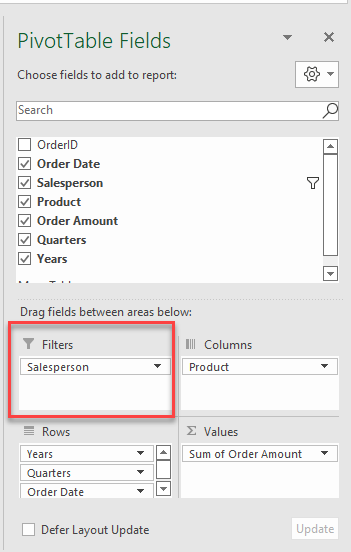
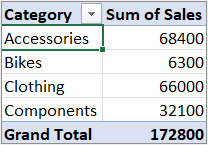
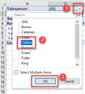
- You can then filter your pivot table by the field(s) from the Filters area (here, Salesperson). Find the filter field(s) at the top of your pivot table, above column headings and a blank row. Click the arrow for the filter field and choose the item to filter on (e.g., Collins). Then click OK.
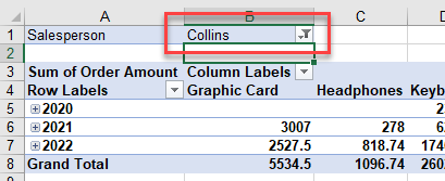
Now the pivot table shows all the information set up in the PivotTable Fields window, but only for rows where the Salesperson is Collins.
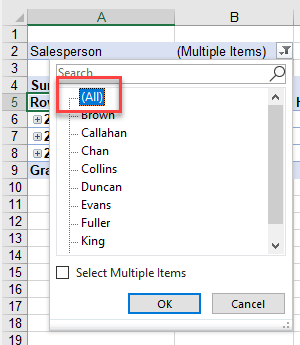
- To clear the filter, click the filter drop down on the right side of the cell. Choose (All) then click OK.
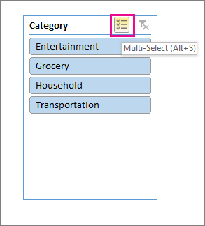
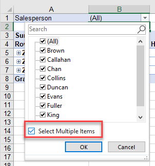
- If you want to filter on multiple items, tick Select Multiple Items. Notice how each item in the drop down now has a checkbox next to it.
- Uncheck the (All) box and tick the items you wish to filter on (e.g., Chan and Collins). Click OK.
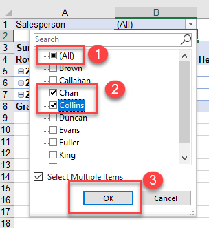
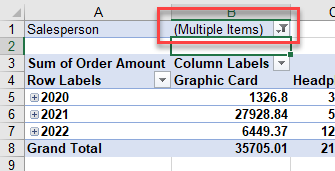
The cell with the filter drop down (here, B1) shows that multiple items are included, but you cannot see which items without clicking the arrow on the right.
- To clear the filter once again, choose (All) from the filter drop down and click OK.
Filter by Row / Column
You can also filter by the row and column labels.
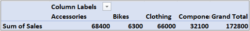
- Click the filter drop down to the right of the Column Labels heading. Remove the checkmark from (Select All), and then tick the item you wish to filter on.
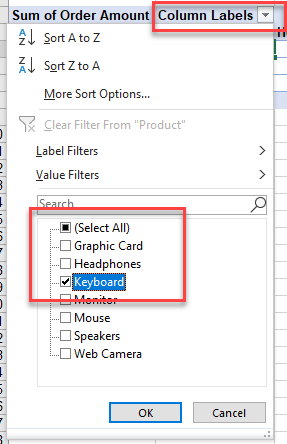
- Click OK to apply the filter.
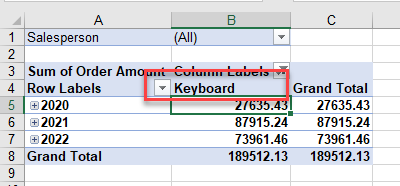
Filter Row Labels in the same way.
Filter Values by Date
If you have dates in your pivot table, you can filter by these dates. This can be done in the Filters, Rows, and/or Columns areas.
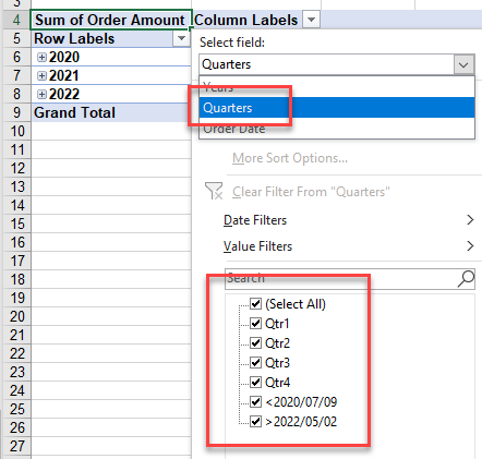
Filter by Year or Quarter
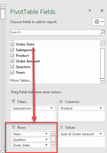
When a date is added to the Rows or Columns area, it is automatically broken down into three groups – Years, Quarters, and the actual value of the date field itself. All three fields are added to the relevant area.
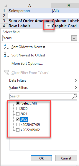
You can then click the Row Labels filter drop down and choose the specific field to filter on (e.g., Years) in the Select field drop down.
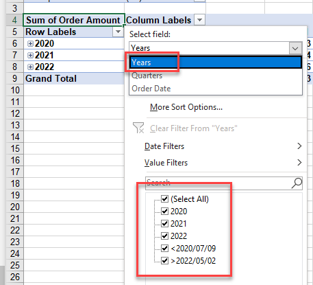
Also try changing the filter field to filter by quarters instead of years.
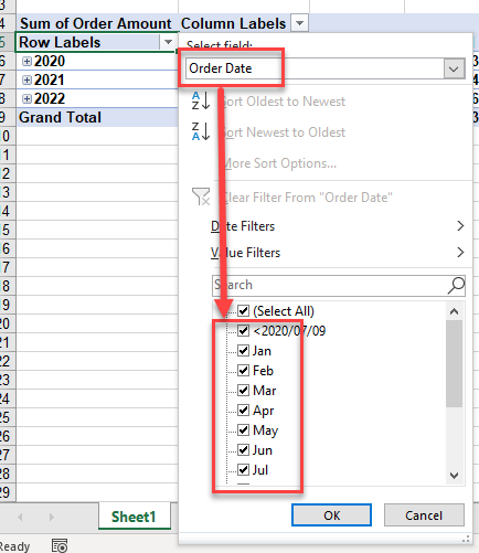
Filter by Month
To filter by month, choose the original field (e.g., Order Date) from the drop down instead of the automatically generated years or quarters.
Other Date Filters
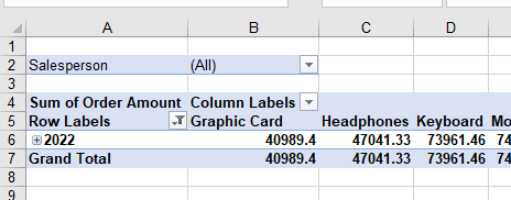
You can also choose Date Filters from the Row Labels drop down, and then choose the criteria you need – for example, This Year.
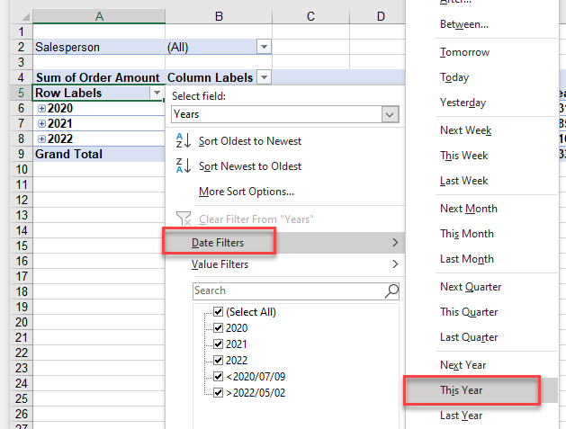
This immediately restricts the data shown to this year only.
Date Range
You can also be more specific and choose the start and end dates to filter on.
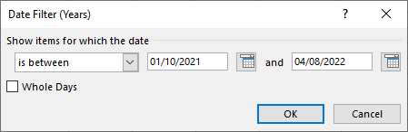
- From the Row Labels drop down, go to Date Filters > Between…
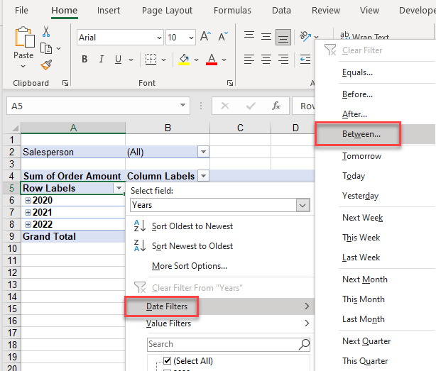
- Select the start and end dates and click OK.
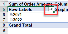
Notice a small icon in the Row Labels drop down (on the right side of the cell) indicating that a filter is applied.
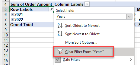
- To get rid of the filter, click Clear Filter from “Years” in the drop down.
Add Additional Filters
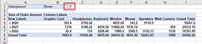
Individual columns of a pivot table do not have filters automatically in place.
- To create a filter on these values, select the cell to the right of the pivot table (here, J5), and then in the Ribbon, go to Home > Editing > Filter.
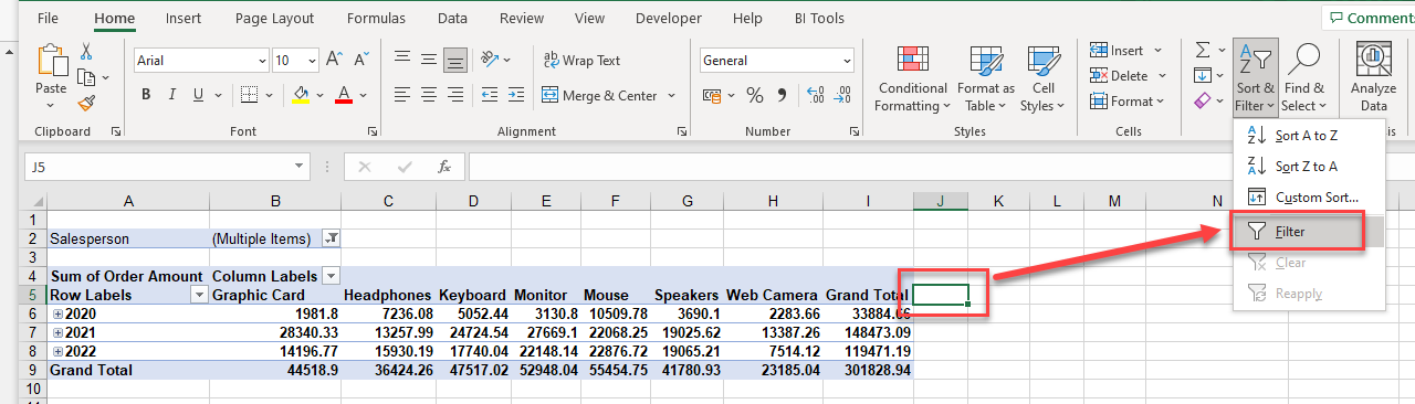
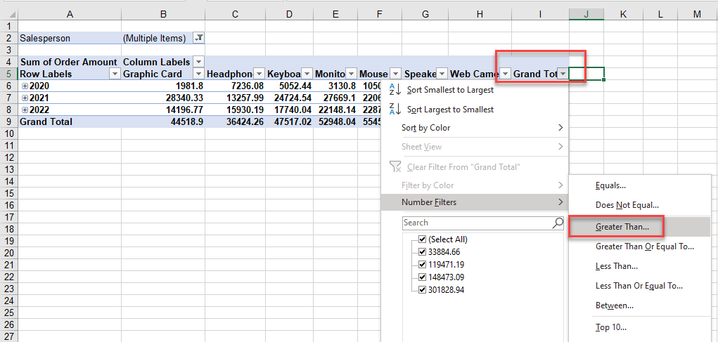
- This adds a filter to each column label. You can then filter on each value. For example, you can tick any of the individual values in the Grand Total list, or you can use a Number Filter, such as one that includes only values Greater Than a certain amount.
Tip: Try using some shortcuts when you’re working with pivot tables.
Filter Pivot Table in Google Sheets
Pivot tables, especially the window where the table is built and structured, look a little different in Google Sheets, but the methods for filtering are similar.
- In the Pivot table editor, click Add.
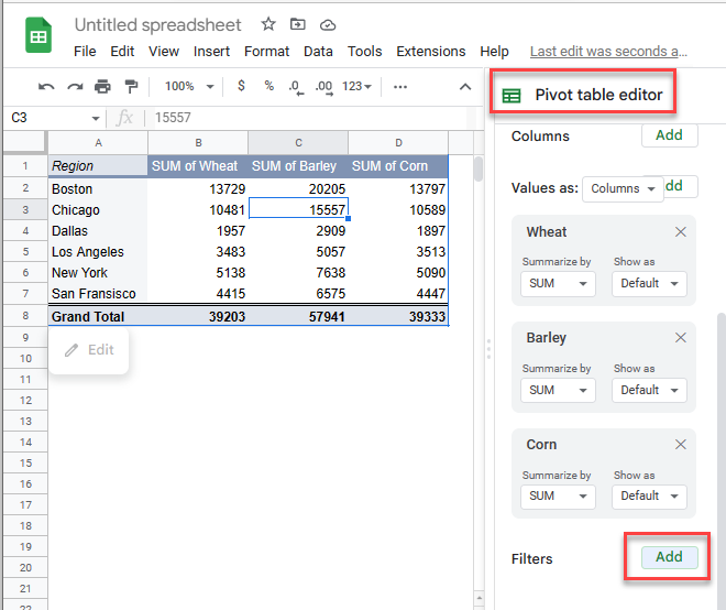
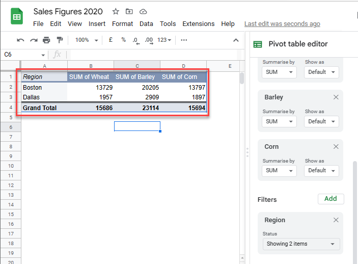
- Choose the field you wish to filter on (e.g., Region).
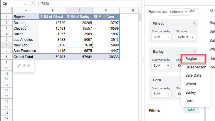
- Under Filter by values, click Clear. Then individually tick the values to include in the filter.
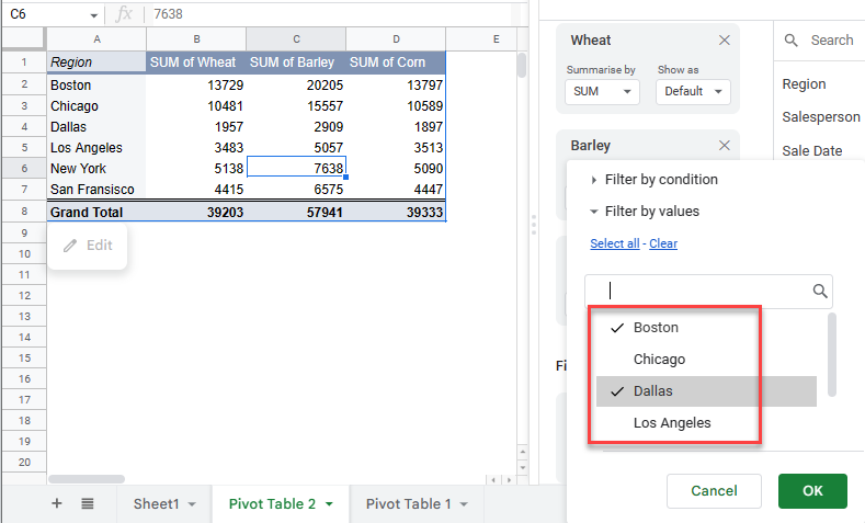
- Click OK to apply the filter.
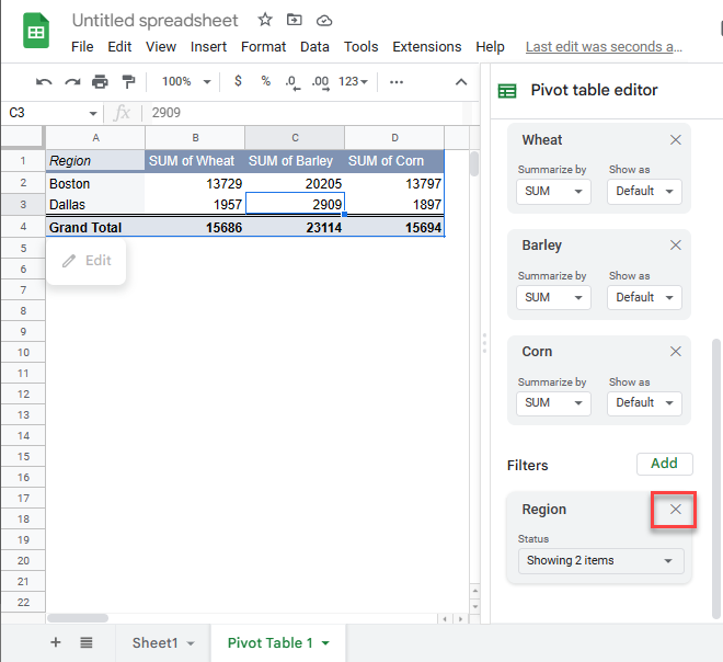
- To clear the filter, click the X to the right of the filtered field.
Filter by Condition
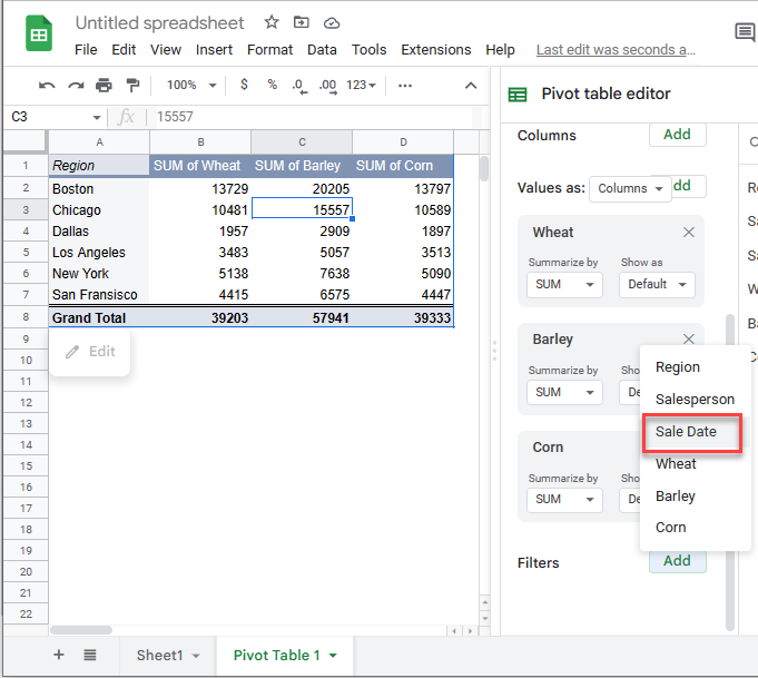
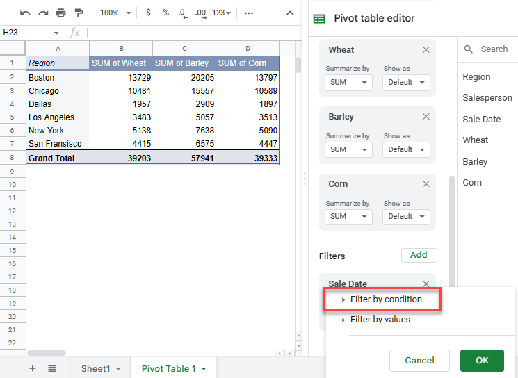
- Now, add a filter for the Sale Date to the pivot table.
- Click Filter by condition.
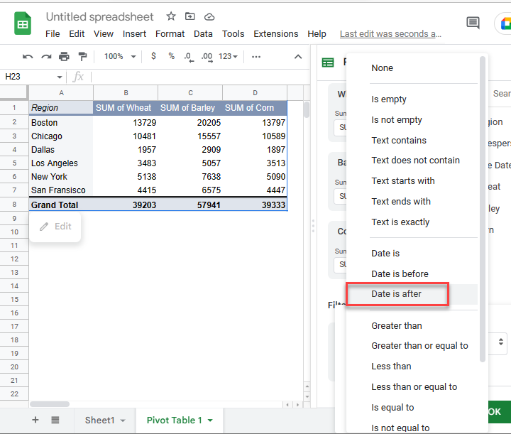
- Choose Date is after from the drop down.
- Then, click exact date from the next drop down.
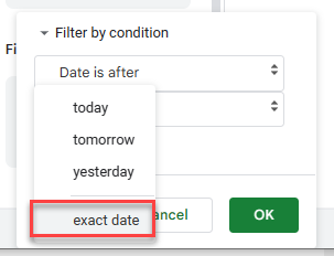
- In the bottom box, type in the date you need. Click OK.

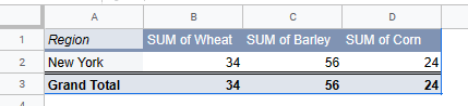
The pivot table is filtered accordingly.
The Pivot Table is a powerful tool for Microsoft Excel. With its help the user analyzes large ranges and sums up just in a few clicks. He can display only the information that he need at this very moment.
Filter in the Excel Pivot Table
You can convert almost any range of data in the Pivot Table: the results of financial transactions, information about suppliers and buyers, the home library catalog, etc.
For example, take the following table:
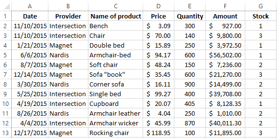
We will create a summary table: «INSERT» — «PivotTable». Put it on a new sheet.
We added information about suppliers including quantity and cost. Now it’s in our consolidated report.
Let’s remind how the summary report dialog box looks like:
We set the program instructions to generate a summary report while dragging the headers. If you accidentally make an error, you can delete the header from the bottom area or replace it with another one.
Totals appears according to the data which are placed in the field «Values». In automatic mode it’s the sum. But you can set «average», «maximum», etc. If you need to do this for the values of the entire field, then click on the name of the column and change the way the totals are presented:
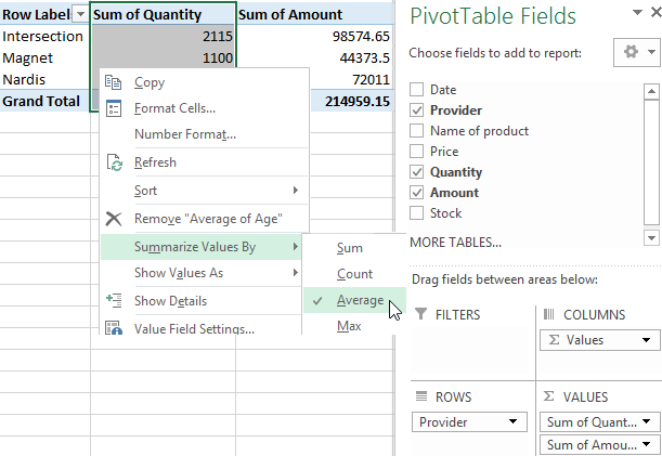
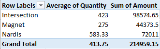
For example, the average number of orders for each supplier:
Results can be changed not in all columns but only in a separate cell. Then we right-click on this cell.
Set the filter in the summary report:
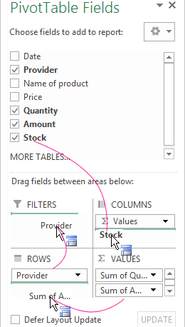
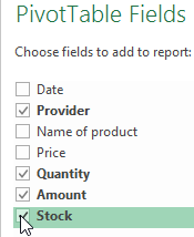
- Put a tick in front of the «Stock» header in the list of fields to add to the table filters we need.
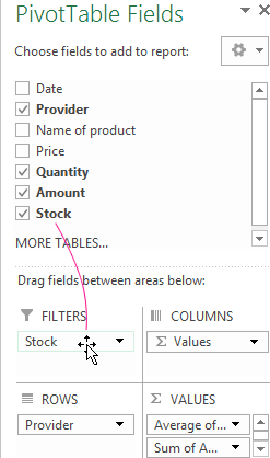
- Drag this field to the «FILTERS» area.
- The table became three-dimensional and the «Stock» tag turn up at the top.
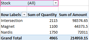
Now we can filter the values in the report by warehouse number. Click on the arrow in the right corner of the cell and select the items we are interested in:
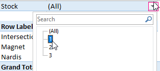
For example, «1»:
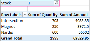
The report displays information only for the first warehouse. We see above the value and the icon of the filter.
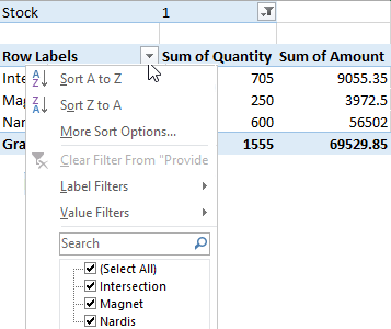
You can also filter the report using the values in the first column.
Sorting in the Excel Pivot Table
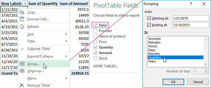
Let’s transform our consolidated report: we will remove the value «Suppliers» and add the «Date» tag.
Let’s make the table more useful. We will group the dates by quarters. To do this right-click on any cell with a date. In the drop-down menu select «Group». Fill in the grouping parameters:
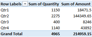
The Pivot Table takes the following form after clicking OK:
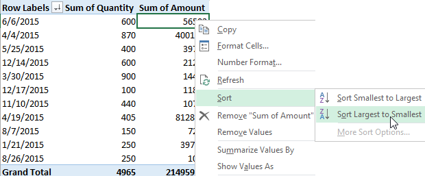
Let’s sort the data in the report by the value of the column «Amount». Click the right mouse button on any cell or column name. Select «Sort» and sorting method.
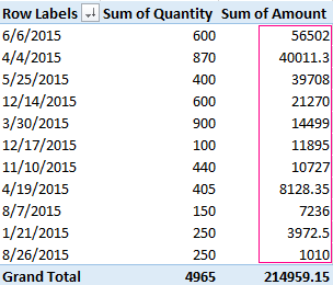
The values in the summary report will be changed according to the sorted data:
Now let’s sort the data by date. Click right mouse button and choose «Sort». You can select the sorting method and stop with this step. But we will follow an otherwise pathway. Click «More Sort Options»-«More Options…». A window like this will open:
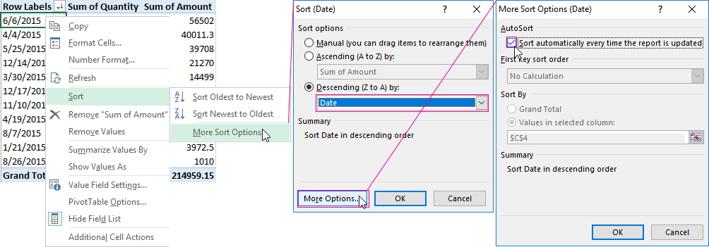
Let’s set sorting parameters: «Sort Date in descending order». Click on the «More Options» button. Put a checkmark next to «AutoSort»-«Sort automatically every time the report is updated».
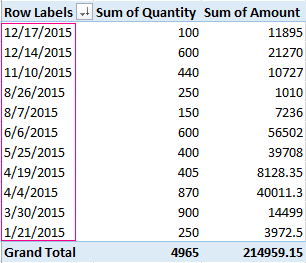
Now Excel will sort dates in descending order (from new to old) when the new dates will appear in the Pivot Table:
Formulas in Excel Pivot Table
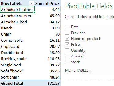
Firstly, we will compile a consolidated report, where the totals will be presented not only by the sum. Let’s start from scratch with an empty table. For one we learn how to add a column in the Pivot Table.
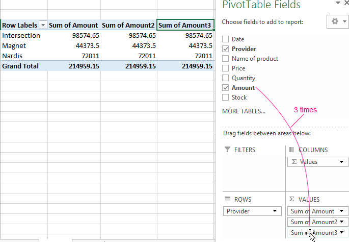
- Add the «Provider» header to the report. We will drag «Amount» header for three times in the «Value» field. Now three identical columns will be added to the Pivot Table.
- Leave the value «Sum» for totals in the first column. For the second one choose «Average». For the third one set «Count».
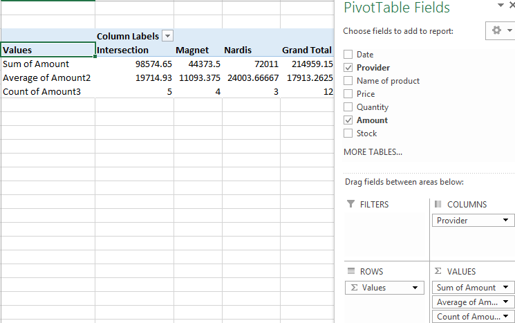
- We swap column values and row values. «Provider» goes to the column names. «Σ values» goes to the lines names.
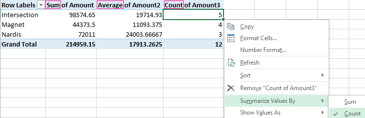
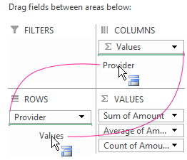
The consolidated report became more convenient for perception:
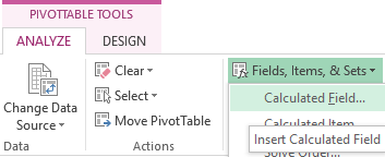
Let’s study how to prescribe formulas in a summary table. Click on any cell in the report to activate the «PIVOTTABLE TOOLS» tool.
On the «ANALYZE» tab we select «Fields, Items and Sets» — «Calculated Field».
Click and a dialog box opens. Enter the name of the calculated area and the formula to find the values.
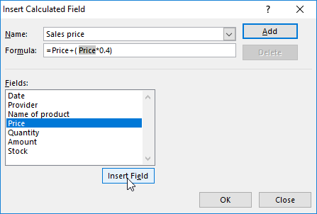
We get the added additional column with the result of calculations using the formula.
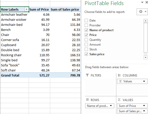
Download Pivot Table example
Make an experiments: summary table tools are hothouse. You can always delete the unsuccessful version and redo it If something does not work out.