Filter with function excel

The FILTER function allows you to filter a range of data based on criteria you define.

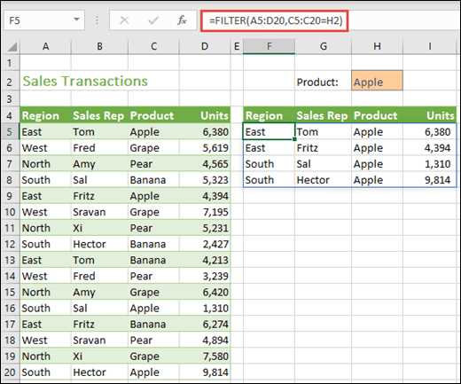
In the following example we used the formula =FILTER(A5:D20,C5:C20=H2,»») to return all records for Apple, as selected in cell H2, and if there are no apples, return an empty string («»).

The FILTER function filters an array based on a Boolean (True/False) array.

=FILTER(array,include,[if_empty])

Argument	Description
array Required	The array, or range to filter
include Required	A Boolean array whose height or width is the same as the array
[if_empty] Optional	The value to return if all values in the included array are empty (filter returns nothing)

Notes: 

• An array can be thought of as a row of values, a column of values, or a combination of rows and columns of values. In the example above, the source array for our FILTER formula is range A5:D20.

• The FILTER function will return an array, which will spill if it’s the final result of a formula. This means that Excel will dynamically create the appropriate sized array range when you press ENTER. If your supporting data is in an Excel table, then the array will automatically resize as you add or remove data from your array range if you’re using structured references. For more details, see this article on spilled array behavior.

• If your dataset has the potential of returning an empty value, then use the 3rd argument ([if_empty]). Otherwise, a #CALC! error will result, as Excel does not currently support empty arrays.

• If any value of the include argument is an error (#N/A, #VALUE, etc.) or cannot be converted to a Boolean, the FILTER function will return an error.  

• Excel has limited support for dynamic arrays between workbooks, and this scenario is only supported when both workbooks are open. If you close the source workbook, any linked dynamic array formulas will return a #REF! error when they are refreshed.

Examples

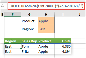
FILTER used to return multiple criteria

In this case, we’re using the multiplication operator (*) to return all values in our array range (A5:D20) that have Apples AND are in the East region: =FILTER(A5:D20,(C5:C20=H1)*(A5:A20=H2),»»).

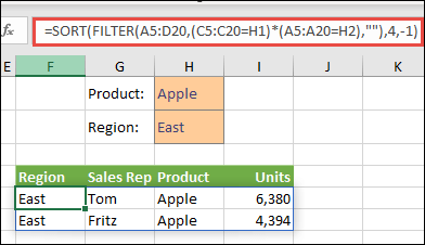
FILTER used to return multiple criteria and sort

In this case, we’re using the previous FILTER function with the SORT function to return all values in our array range (A5:D20) that have Apples AND are in the East region, and then sort Units in descending order: =SORT(FILTER(A5:D20,(C5:C20=H1)*(A5:A20=H2),»»),4,-1)

In this case, we’re using the FILTER function with the addition operator (+) to return all values in our array range (A5:D20) that have Apples OR are in the East region, and then sort Units in descending order: =SORT(FILTER(A5:D20,(C5:C20=H1)+(A5:A20=H2),»»),4,-1).

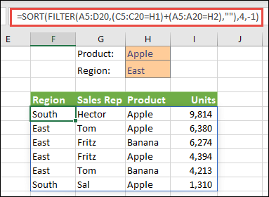
Notice that none of the functions require absolute references, since they only exist in one cell, and spill their results to neighboring cells.

Need more help?

You can always ask an expert in the Excel Tech Community or get support in the Answers community.

See Also

RANDARRAY function

SEQUENCE function

SORT function

SORTBY function

UNIQUE function

#SPILL! errors in Excel

Dynamic arrays and spilled array behavior

Implicit intersection operator: @

The FILTER function «filters» a range of data based on supplied criteria. The result is an array of matching values from the original range. In plain language, the FILTER function will extract matching records from a set of data by applying one or more logical tests. Logical tests are supplied as the include argument and can include many kinds of formula criteria. For example, FILTER can match data in a certain year or month, data that contains specific text, or values greater than a certain threshold.

The FILTER function takes three arguments: array, include, and if_empty. Array is the range or array to filter. The include argument should consist of one or more logical tests. These tests should return TRUE or FALSE based on the evaluation of values from array. The last argument, if_empty, is the result to return when FILTER finds no matching values. Typically this is a message like «No records found», but other values can be returned as well. Supply an empty string («») to display nothing.

The results from FILTER are dynamic. When values in the source data change, or the source data array is resized, the results from FILTER will update automatically. Results from FILTER will «spill» onto the worksheet into multiple cells.

Basic example

To extract values in A1:A10 that are greater than 100:

=FILTER(A1:A10,A1:A10>100)

To extract rows in A1:C5 where the value in A1:A5 is greater than 100:

=FILTER(A1:C5,A1:A5>100)

Notice the only difference in the above formulas is that the second formula provides a multi-column range for array. The logical test used for the include argument is the same.

Note: FILTER will return a #CALC! error if no matching data is found

Filter for Red group

In the example shown above, the formula in F5 is:

=FILTER(B5:D14,D5:D14=H2,"No results")

Since the value in H2 is «red», the FILTER function extracts data from array where the Group column contains «red». All matching records are returned to the worksheet starting from cell F5, where the formula exists.

Values can be hardcoded as well. The formula below has the same result as above with «red» hardcoded into the criteria:

=FILTER(B5:D14,D5:D14="red","No results")

No matching data

The value for is_empty is returned when FILTER does not find matching results. If a value for if_empty is not provided, FILTER will return a #CALC! error if no matching data is found:

=FILTER(range,logic) // #CALC! error

Often, is_empty is configured to provide a text message to the user:

=FILTER(range,logic,"No results") // display message

To display nothing when no matching data is found, supply an empty string («») for if_empty:

=FILTER(range,logic,"") // display nothing

Values that contain text

To extract data based on a logical test for values that contain specific text, you can use a formula like this:

=FILTER(rng1,ISNUMBER(SEARCH("txt",rng2)))

In this formula, the SEARCH function is used to look for «txt» in rng2, which would typically be a column in rng1. The ISNUMBER function is used to convert the result from SEARCH into TRUE or FALSE. Read a full explanation here.

Filter by date

FILTER can be used with dates by constructing logical tests appropriate for Excel dates. For example, to extract records from rng1 where the date in rng2 is in July you can use a generic formula like this:

=FILTER(rng1,MONTH(rng2)=7,"No data") 

This formula relies on the MONTH function to compare the month of dates in rng2 to 7.  See full explanation here.

Multiple criteria

At first glance, it’s not obvious how to apply multiple criteria with the FILTER function. Unlike older functions like COUNTIFS and SUMIFS, which provide multiple arguments for entering multiple conditions, the FILTER function only provides a single argument, include, to target data. The trick is to create logical expressions that use Boolean algebra to target the data of interest and supply these expressions as the include argument. For example, to extract only data where one value is «A» and another is greater than 80, you can use a formula like this:

=FILTER(range,(range="A")*(range>80),"No data")

The math operation of addition (*) joins the two conditions with AND logic: both conditions must be TRUE in order for FILTER to retrieve the data. See a detailed explanation here.

Complex criteria

To filter and extract data based on multiple complex criteria, you can use the FILTER function with a chain of expressions that use boolean logic. For example, the generic formula below filters based on three separate conditions: account begins with «x» AND region is «east», and month is NOT April.

=FILTER(data,(LEFT(account)="x")*(region="east")*NOT(MONTH(date)=4))

See this page for a full explanation. Building criteria with logical expressions is an elegant and flexible approach that can be extended to handle many complex scenarios. See below for more examples.

Notes

1. FILTER can work with both vertical and horizontal arrays.
2. The include argument must have dimensions compatible with the array argument, otherwise FILTER will return #VALUE!
3. If the include array includes any errors, FILTER will return an error.

Filtering is a common everyday action for most Excel users. Whether using AutoFilter or a Table, it is a convenient way to view a subset of data quickly. Until the FILTER function in Excel was released, there was no easy way to achieve this with formulas. When Microsoft announced the changes to Excel’s calculation engine, they also introduced a host of new functions. One of those new functions is FILTER, which returns all the cells from a range that meet specific criteria.

At the time of writing, the FILTER function is only available in Excel 365, Excel 2021 and Excel Online. It will not be available in Excel 2019 or earlier versions.

Download the example file: Click the link below to download the example file used for this post:

Watch the video:

Watch the video on YouTube

Arguments of the FILTER function

Before we look at the arguments required for the FILTER function, let’s look at a basic example to appreciate what it does.

Here the FILTER function returns all the values in cells B3-B10 where the number of characters is greater than 15. Not a scenario that many of us will need, but it perfectly demonstrates the power of the new FILTER function.

FILTER has three arguments:

=FILTER(array, include, [if_empty])

• array: The range of cells, or array of values to filter.
• include: An array of TRUE/FALSE results, where only the TRUE values are retained in the filter.
• [if_empty]: The value to display if no rows are returned.

Examples of using the FILTER function

The following examples illustrate how to use the FILTER function.

Example 1 – FILTER returns an array of rows and columns

In this example, cell F3 contains a single formula, but this formula returns an array of values into the neighboring rows and columns.

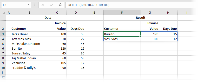
The formula in cell F3 is:

=FILTER(B3:D10,C3:C10>100)

This single formula is returning 2 rows and 3 columns of data where the values in C3-C10 are higher than 100.

Example 2 – #CALC! error caused by the FILTER function

The screenshot below displays what happens when the result of the FILTER function has zero results; we get the #CALC! error.

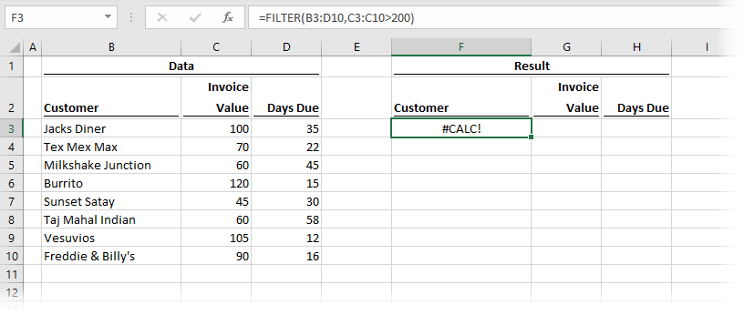
The formula in cell F3 is:

=FILTER(B3:D10,C3:C10>200)

As no rows meet the criteria of Invoice Value being higher than 200, the FILTER cannot return a value, so the #CALC! error is displayed.

Thankfully, Microsoft has given us the if_empty argument, which displays a message if there are no rows returned.

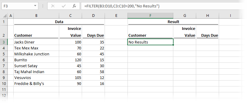
The formula in cell F3 is:

=FILTER(B3:D10,C3:C10>200,"No Results")

In the screenshot above, No Results displays instead of the #CALC! error.

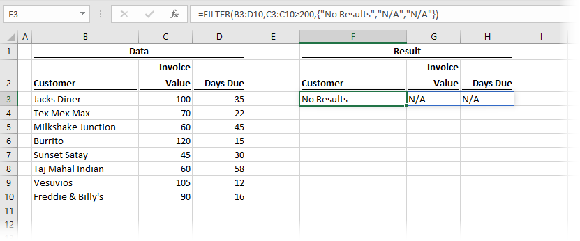
If we wanted to display a result in each column, we could include a constant array within the if_empty argument. The following shows n/a in the Invoice Value and Days Due columns.

=FILTER(B3:D10,C3:C10>200,{"No Results","n/a","n/a"})

This formula would result in the following:

Example 3 – FILTER expands automatically when linked to a table

This example shows how the FILTER function responds when linked to an Excel table.

The FILTER is set to show items where Invoice Value is higher than 100. New records added to the Table which meet the criteria are automatically added to the spill range of the function. Amazing stuff!

Example 4 – Using FILTER with multiple criteria.

Example 4 shows how to apply FILTER with multiple criteria.

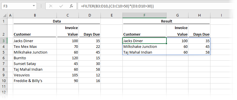
The formula in cell F3 is:

=FILTER(B3:D10,(C3:C10>50)*(D3:D10>30))

For anybody who has used the SUMPRODUCT function, this method of applying multiple conditions will be familiar. Multiplication creates AND logic (i.e., all the criteria must be TRUE). The example above shows where the Invoice Value is greater than 50 and the Days Due is greater than 30.

Addition creates OR logic (i.e., any individual condition can be TRUE).

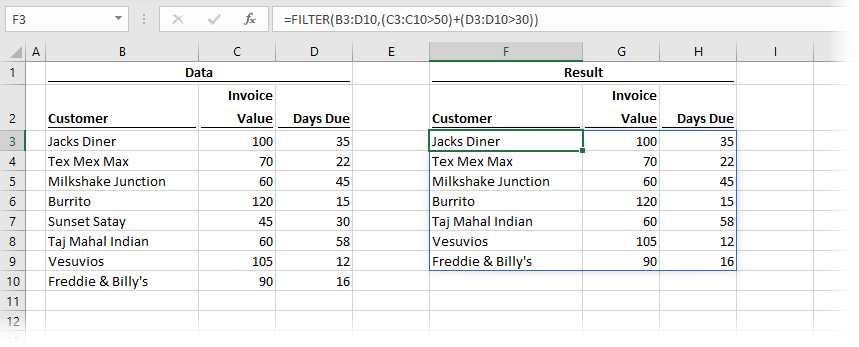
The formula in cell G3 is:

=FILTER(B3:D10,(C3:C10>50)+(D3:D10>30))

The example above shows where the Invoice Value is greater than 50 or the Days Due is greater than 30.

Example 5 – Using FILTER for dependent dynamic drop-down lists

Drop-down lists are a data validation technique. Dependent drop-down lists are an advanced technique where the lists change depending on the result of another cell. For example, if the first drop-down list displays country names, the second drop-down list should only display cities that exist in that country. In Excel 2019 and before there are only tedious methods to achieve this effect, but the new FILTER function makes this super easy.

The formula in cell H3 is:

=UNIQUE(B3:B10)

The UNIQUE function creates a unique list to populate the drop-down in cell F4.

The formula in cell I3 is:

=FILTER(C3:C10,B3:B10=F4)

Depending on the value in cell F4, the values returned by the FILTER function change. The second drop-down in cell F6 changes dynamically based on the value in Cell F4.

Example 6 – Using FILTER with other functions

In this final example, FILTER is nested inside the SORT function.

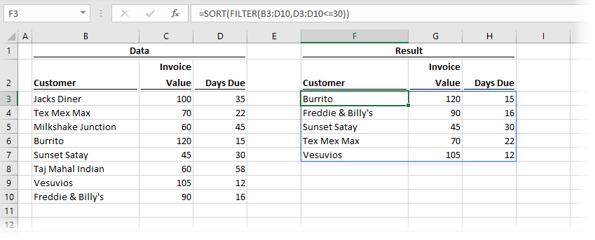
The formula in cell F3 is:

=SORT(FILTER(B3:D10,D3:D10<=30))

First, the FILTER function returns the cells based on the Days Due being less than or equal to 30. The SORT function then puts the Customers into ascending alphabetical order.

Example 7 – Using FILTER to show matching items from a list

How can we match a list of items that could have an unknown size? We can’t keep updating our FILTER function by adding and removing criteria. And, if we had a lot of items to match, it would soon become unmanageable. So, let’s see how we can solve this.

In the example below, the formula in cell H3 returns only the customers listed in F3:F4.

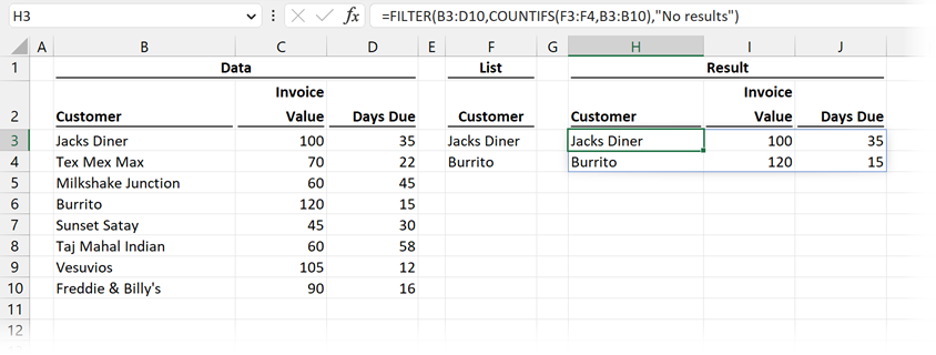
The formula in cell H3 is:

=FILTER(B3:D10,COUNTIFS(F3:F4,B3:B10),"No results")

The COUNTIFS function returns a positive number if the item exists in both the data and the list, or zero if it exists in only one. Since positive numbers are always TRUE and zeros are always FALSE, this provides the TRUE/FALSE logic required for the FILTER function to return only the matching items.

NOTE: If the list starting in F3 were generated by another array formula, or by Power Query this solution would be completely dynamic (that is outside the scope of the current post, so we have used static ranges for this example).

Example 8 – Simulating wildcard search with FILTER

The FILTER function does not allow wildcard characters in the criteria. However, by using a combination of SEARCH and ISNUMBER we can simulate a similar effect.

In the example below, the formula in cell H3 returns only the items where the customer name contains the letters in cell F3.

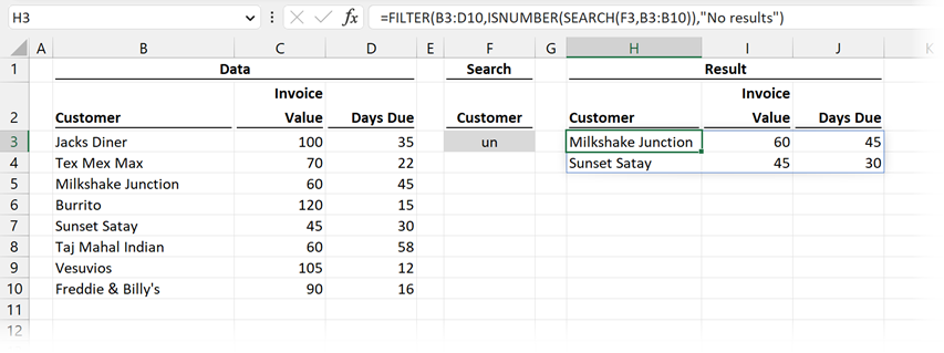
The formula in cell H3 is:

=FILTER(B3:D10,ISNUMBER(SEARCH(F3,B3:B10)),"No results")

SEARCH returns a number if the search term in cell F3 is found in each value in B3-B10.

ISNUMBER returns TRUE or FALSE for each value depending on if SEARCH returns a number. This TRUE/FALSE value provides the logic needed by FILTER to return the matching items.

In this scenario only, Milkshake Junction and Sunset Satay contain un as a substring, therefore only these customers are returned.

Want to learn more?

There is a lot to learn about dynamic arrays and the new functions. Check out my other posts here to learn more:

• Introduction to dynamic arrays – learn how the excel calculation engine has changed.
• UNIQUE – to list the unique values in a range
• SORT – to sort the values in a range
• SORTBY – to sort values based on the order of other values
• FILTER – to return only the values which meet specific criteria
• SEQUENCE – to return a sequence of numbers
• RANDARRAY – to return an array of random numbers
• Using dynamic arrays with other Excel features – learn to use dynamic arrays with charts, PivotTables, pictures etc.
• Advanced dynamic array formula techniques – learn the advanced techniques for managing dynamic arrays

The FILTER function is an Excel function that lets you fetch or «filter» a data set based on the criteria supplied via an argument. The FILTER function was introduced in Office 365 and will not be accessible in Office 2019 or earlier versions.

FILTER is an in-built worksheet function and belongs to Excel’s new Dynamic Arrays function category. The FILTER function returns an array of values that are spilled onto your worksheet unless the function is nested to relay the output to another function.

FILTER is a dynamic function. This means when you alter the values in the source data or resize the source data array, the Excel FILTER function will automatically update the returned values.

Syntax

The syntax of the Filter function is as follows:

=FILTER(array, include, [if_empty])

Arguments:

array – This is a required argument where you specify the range or array that you want to filter.
include – This is a required argument where you supply the filtering criteria as a Boolean array.
if_empty – This is an optional argument where you specify a value that the function should return if none of the entries meet the supplied criteria.

Important Characteristics of the FILTER function

• You can use the FILTER function for filtering both horizontal as well as vertical arrays.
• When you use the FILTER function between two separate workbooks, ensure that both of them are open. If they are not, the function will return a #REF! error.
• Since the FILTER function spills the output (assuming your data is so organized), ensure that you have sufficient empty cells to the right and below. If you do not, the function will return a #SPILL error.
• The FILTER function returns a #VALUE! error if the dimensions supplied in the include argument are incompatible with the array argument.
• The FILTER function was introduced in Office 365 and is not available in Office 2019 or earlier version.

Examples of the FILTER function

Let’s have a look at the examples of the FILTER function:

Example 1 – Plain-vanilla Version of the Filter function

Suppose we want a list of students that have Grade «A» in the data set.

In order to do this, we will input the entire data set, i.e., A2:C16, in the array argument.

In the include argument, we will input C2:C16=»A» which will produce a Boolean array that assigns TRUE for all ‘A’s.

The last argument (if_empty) is an optional string where you will let the formula know what it should return if it does not find any values. In our case, we use a text string «No matches», but you could also have the formula return nothing by passing an empty string («»).

So the final formula would be –

=FILTER(A2:C16,C2:C16="A","No matches")

If you prefer, you could also have a cell reference instead of adding a character or a text string in the include argument. For example, let’s say you write «A» in cell G6 and then input the include argument as C3:C17=G6.

So the formula would be –

=FILTER(A2:C17,C2:C17=G6,"No matches")

The FILTER function will also work smoothly for horizontally organized data sets. Just ensure that the width of ranges defined in the array and include arguments are the same.

Also, in case of no matching records the formula, returns the string no match as shown.

Since none of the students in the above dataset has Grade «D», the result is the «No matches» string.

Example 2 – FILTER function Used in Combination With the EXACT function

Nesting the EXACT function inside the FILTER function enables you to fetch an exact, case-sensitive match.

=FILTER(A2:C16,EXACT(A2:A16,"Bing"),"No matches")

The EXACT function has a simple role here and works as the include argument in the FILTER function. EXACT returns TRUE for an exactly matching string and FALSE otherwise. As such, the EXACT function will return 15 Boolean values (for each cell in the B2:B16 range), which in our case will look something like this:

{FALSE; FALSE; FALSE; FALSE; TRUE; FALSE; FALSE; FALSE; FALSE; FALSE; FALSE; FALSE; FALSE; FALSE; FALSE}

At position 5, «Bing» is the only match and hence returns TRUE.

This array is relayed to the FILTER function as the include argument. Next, FILTER uses the array returned by EXACT to return only those rows that contain the string «Bing» (i.e., rows that have been assigned a TRUE value by the EXACT function).

Note: Please note that we can also get to the same output by just adding the condition (A2:A16)=»Bing» in the include argument, but in that case, the search will be case-insensitive.

Example 3 – Filtering with Wildcards Using the FILTER function

Let’s discuss some big-boy formulas now. The FILTER function does not in itself support wildcard characters, but we can input a logical test in the include argument to get the output we want.

We will nest the ISNUMBER and SEARCH functions, like so:

=FILTER(A2:A16,ISNUMBER(SEARCH("G*",A2:A16)),"No matches")

Let’s walk through each component of the formula and see what role they play. We will work out the SEARCH function’s output first. The search function is looking for any string in column A that has the letter «G». We have 3 last names that contain a G – Bing, Geller, and Green. Remember, that search function only returns the position of the searched character.

Therefore, wherever the SEARCH function finds a G, it will return a number (i.e., the position of G), while for others, you will get a #VALUE! error. If you want to perform a case-sensitive SEARCH, you can replace the SEARCH function with the FIND function. Let’s replace the SEARCH function’s return in our formula:

=FILTER (A2:A16, ISNUMBER ({#VALUE!, #VALUE!, #VALUE!, #VALUE!, 4, 1, 1, #VALUE!, #VALUE!, #VALUE!, #VALUE!, #VALUE!, #VALUE!, #VALUE!, #VALUE!), "No matches")

Next, we have the ISNUMBER function. ISNUMBER function has a simple role to play. It will look at the SEARCH function’s return and assign TRUE for results that are a number and FALSE for results that are not a number (i.e., are a #VALUE! error in our case).

If you follow what is happening in the formula so far, the remaining part is a cakewalk. The ISNUMBER function relays this output (i.e., 3 TRUEs for the numbers and 12 FALSEs for the #VALUE! errors) to the FILTER function. The FILTER function will then let only those data points make it to the final output, for which the result was TRUE.

So, as our final output, we should have 3 names – Bing, Geller, and Green.

Example 4 – FILTER function With Multiple Criteria (AND/OR operator)

We have so far not used the Scores column from our data set. Let’s remedy that, shall we?

So, here we are trying to find the students who have Grade «A» and a score of above 100.

We will first use the AND criteria, with an asterisk (*). To do this, we will extend the include argument using Boolean logic, like so:

=FILTER(A2:C16,(C2:C16=G6)*(B2:B16>100),"No matches")

Using the ‘*’ multiplies the Boolean values, where True equals 1, and False equals 0. So, when the expressions inside the parentheses are multiplied in the formula, there are two possibilities:

• You get a FALSE (or a 0): If the expressions inside both the parentheses return False (0*0) or one of them returns FALSE (0*1).
• You get a TRUE (or a 1): If the expressions inside both the parentheses return TRUE (1*1).

Therefore, when the first parenthesis finds an A and returns TRUE and the second parenthesis finds the score to be greater than 100 and returns TRUE as well, we will have our return (or get the string «No matches»). Using logical expressions like this is an efficient approach to filter criteria.

Much the same way, we can use the OR criteria by using a plus (+) between two parentheses in the include argument, like so:

=FILTER(A2:C16,(C2:C16=G6)+(B2:B16>100),"No matches")

This will get us all the students who either have Grade «A» or scores greater than 100.

Similar to what we saw for the AND criteria, we can get two possible outcomes when Boolean values in the include argument are added:

• You get a FALSE (or a 0): If the expressions inside both parentheses return a FALSE (0+0).
• You get a TRUE (or a 1): If the expression inside one of the parenthesis returns a TRUE (0+1) or both parentheses return a TRUE (1+1).

Wait, if both parentheses return 1, it will add up to 2, right?

Fortunately, that does not matter. Excel will consider anything that is 0 as FALSE, anything that is not 0 as TRUE.

This is how you can incorporate the AND or OR criteria in your formulas.

Example 5 – Filtering Duplicates Using the FILTER and COUNTIFS functions

If your data set is massive, it is quite likely that you may need to deal with duplicates. When a data point has more than a single instance, we can filter the duplicate instances by using a nested formula, like so:

=FILTER(A2:C20,COUNTIFS(A2:A20,A2:A20,B2:B20,B2:B20,C2:C20,C2:C20)>1,"No matches")

Essentially, we are using the COUNTIFS function to count the instances of data points and extracting those data points that occur more than once. By nesting the COUNTIFS function in the include argument, you are instructing the FILTER formula to include only those results that occur more than once (>1).

You can add or remove the number of columns passed to the COUNTIFS function for filtering duplicate data based on your own requirements.

The FILTER function will spill the return with duplicate instances into a range of cells, as shown in the image.

Recommended Reading: How to find duplicates in excel

Example 6 – Filtering Blank Records Using the FILTER function

We will revisit what we learned in a previous example where we discussed the use of AND criteria using an ‘*’. We will use a <> operator (i.e., not equal to) inside the parenthesis to check if a cell has an empty string («»), like so:

=FILTER(A2:C16,(A2:A16<>"")*(B2:B16<>"")*(C2:C16<>""),"No matches")

Here, we are checking the data points contained in the A, B, and C columns and retrieving only those data points that have a value in all three columns. To do this, we instruct Excel to check for empty cells by defining a column and checking for empty cells by adding a ‘<>’ (not equal to) operator and an empty string («»). To add an AND criteria, we will use a ‘*’ between the parenthesis.

If a cell in any of those columns is empty, the return will exclude that particular row entirely.

Example 7 – FILTER function Used in Combination with SUM, MIN, MAX, and AVERAGE functions

The FILTER function packs in a punch. In addition to performing a whole list of tasks discussed above, it is also capable of summarizing the data it returns after filtering.

To accomplish this, we will use the aggregation family of functions – like SUM, MIN, MAX, and AVERAGE.

It is actually pretty straightforward. All we need to do is relay the return from the FILTER function to any of the mentioned aggregation functions, like so:

=SUM(FILTER(B2:B16,C2:C16="A",0)) //Sum of Grade A scores
=MIN(FILTER(B2:B16,C2:C16="A",0)) //Min of Grade A scores
=MAX(FILTER(B2:B16,C2:C16="A",0)) //Max of Grade A scores
=AVERAGE(FILTER(B2:B16,C2:C16="A",0)) //Average of Grade A scores

Here, the FILTER function will include all rows that have the letter «A» and return 0 for rows that do not match. It will then pick up the values that correspond to «A» from column B. These values will be handed over to the aggregation functions, giving us our final output.

Note: It is important to specify the if_empty argument as 0. Using a string like «No matches» will result in a #VALUE! error, since the aggregation functions cannot handle strings in case of non-matching records.

Example 8 – FILTER function to return Non-Adjacent Columns

Let’s say we want just the Name and Score columns of students with Grade «A». How must we explain to the FILTER function that we want just these two columns when they are non-contagious?

While there is no separate formula to do this, we can accomplish this by sprinkling some logic into the FILTER function. We will nest one FILTER formula inside another FILTER formula and use Boolean values in the include argument of the outer FILTER formula to exclude the Names column, like so:

=FILTER(FILTER(A2:C16,C2:C16="A"),{1,0,1})

Let’s put this formula in words.

The nested (inner) FILTER function is just a simple formula, which we are comfortable with by now.

So, let’s jump over to the outer FILTER function.

The nested FILTER function works as the outer FILTER function’s array argument, informing the outer FILTER function that this is where I want the returned values to come from. The include argument is where the magic happens. We use «1, 0, 1» (alternatively, we could use TRUE, FALSE, TRUE) and let the outer FILTER function know that we want to include only the first and third columns.

Simple, isn’t it?

I hope I unraveled all the mysteries surrounding the brand new FILTER function and covered a little more as well. Incorporate these formulas into your worksheets, and you will become a FILTER function ninja in no time. I will see you soon with another intriguing Excel function, until then… sayonara.

This post will guide you how to extracts matched values using FILTER function in Microsoft Excel 365. And also will introduce that how to use FILTER function with same examples in Excel 365.

---

The FILTER function “filters” a set of data according to the conditions specified. The outcome is an array of values that match those in the original range. Simply said, the FILTER function extracts matched records from a collection of data using one or more logical checks. The include argument specifies logical tests, which might encompass a wide variety of formula conditions. For instance, FILTER may match data from a given year or month, data containing specific content, or numbers above a specified threshold.

=FILTER(array,include,[if empty])

Three parameters are required for the FILTER function: array, include, and if empty.

Where:

• Array – This is required argument. The range or array to filter is specified by array.
• Include – This is required argument. Include one or more logical tests in the include These tests should return TRUE or FALSE depending on the array values evaluated.
• If_empty – This is option argument. The last input, if empty, specifies the value to return if FILTER does not discover any matching values. Typically, this is a message along the lines of “No records found,” although other values may also be returned. To show nothing, provide an empty string (“”).

Entering FILTER Formula in Excel

---

FILTER provides dynamic results. When the values in the source data change or the size of the source data array changes, the FILTER results are updated automatically. The results of FILTER will “leak” into numerous cells on the worksheet.

To filter data in Excel using the FILTER function, follow these steps:

Step1: To begin your filter formula, enter =FILTER(.

Step2: Enter the address for the range of cells containing the data you want to filter, for example, A2:C10.

Step3: Type a comma, followed by the filter's condition, such as B2:B20>3 (To specify a condition, type the address of the “criteria column,” such as C1:C, followed by an operator symbol such as greater than (>), and finally the criterion, such as the number 3.

Step4: Complete the parenthesis with a closing parenthesis and then hit enter on the keyboard. Your full formula will appear as follows: =FILTER(A2:C10, B2:B20>3)

I’ll begin with the fundamentals of utilizing the FILTER function, and then demonstrate some more advanced uses of the FILTER function. This article discusses the FILTER function as a formula entered into spreadsheet cells, not the filter command accessible from the toolbar and pop-up menus.

While using the FILTER function in Excel is almost identical to using it in Google Sheets, there are some subtle variations.

Excel filtering by a single criteria

---

To begin, let’s review how to use Excel’s FILTER function in its simplest version, with a single condition/criteria.

I’ll demonstrate how to filter data using a number, a cell value, a text string, or a date… and I’ll also demonstrate how to utilize a variety of “operators” in the filter condition (Less than, Equal to, etc…).

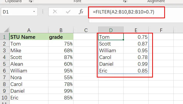
Example 1: How to use a number as a filter

---

In this first demonstration of how to use the filter tool in Excel, we have a list of students and their grades and wish to create a filtered list of only students with flawless grades.

The assignment: Display a list of students and their grades, but only those who have earned an A.

The reasoning: Filter the range A2:B10 for values larger than 0.7 in the column B2:B10 (70 percent ). Then you can use the following FILTER formula,type:

=FILTER(A2:B10, B2:B10 >0.7)

Example 2: How to filter in Excel by a cell value

---

In this excel filter function example, we want to do the same thing as stated before, but rather than inputting the condition straight into the formula, we’re going to use a cell reference.

When you filter in Excel by a cell value, your sheet is configured in such a way that you may alter the value in the cell at any moment, which updates the value to which the filter criterion is tied.

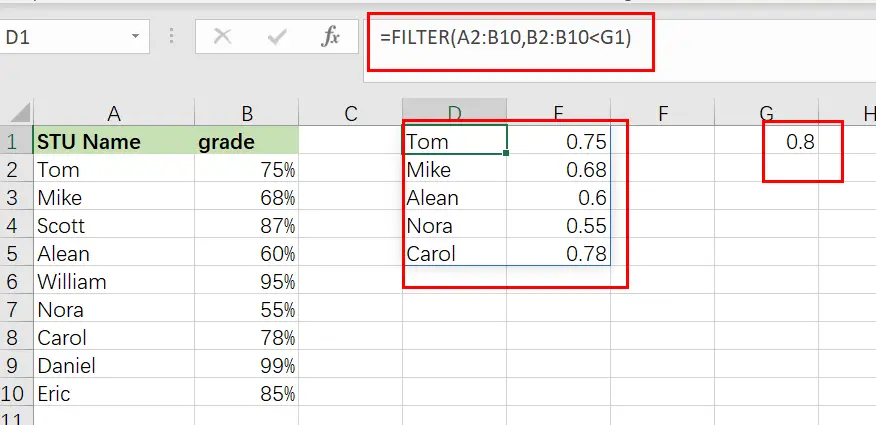
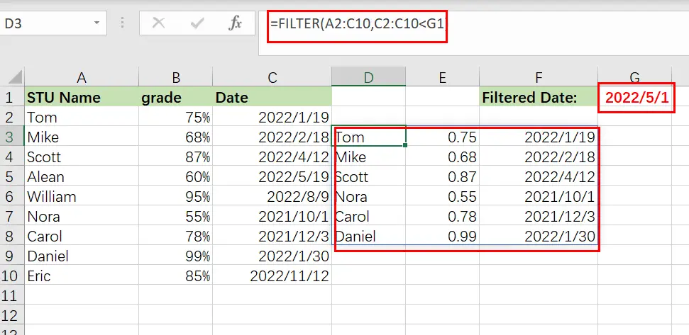
In this example, rather than explicitly entering the value “0.8” into the formula, the filter criterion is set to cell G1, which contains the “0.8” value.

The assignment: Display a list of students and their grades, but only those with a score of less than 80%.

The reasoning: Filter the range A2:B10 to the extent that B2:B10 is smaller than the value supplied in column G1 (0.8).

You can use the following FILTER formula, type:

=FILTER(A2:B10, B2:B10 <G1)

Example 3: Using Excel’s text filter

---

In this example, we’ll utilize a text string as the filter formula’s criterion. This is fairly similar to using a number, except that the text to filter must be enclosed in quote marks.

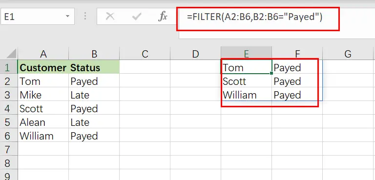
We are filtering a list of customers and their payment status in this instance, and we want to present just customers with a payment status of “Payed“.

The objective is to provide a list of clients that have paid on their payments.

The reasoning: Filter the range A2:B6 by substituting the string “ Payed ” for B2:B6.

The following formula: In this example, the formula below is typed in the cell (E1).

=FILTER(A3:B12, B2:B6=" Payed ")

Example 4: Using NOT EQUAL TO as a FILTER condition in Excel

---

Now that you have a working knowledge of how to use the filter function in Excel, here is another example of filtering by a string of text, but this time we will use the “not equal” operator (<>) to demonstrate how to filter a range and return data that is NOT equal to the criteria you set.

Additionally, we will utilize a bigger data set in this example to show a more comprehensive usage of the FILTER function in the real world.

You may be surprised at how often a circumstance arises in which you need to filter data that is “not equal to” a certain number or piece of text.

In this example, we’ll use a report/spreadsheet to display data from sales calls that occur at your organization, and we’ll filter the data to exclude a certain sales person (Scott) from the result.

The assignment: Display sales call statistics for all sales representatives except ” Scott “.

The reasoning: Filter the range A2:C10 for values A2:A10 that DO NOT match the string “Scott “.

The following formula: In this example, the formula below is typed in the cell (E1).

=FILTER(A2:C10, A2:A10 <>"Scott")

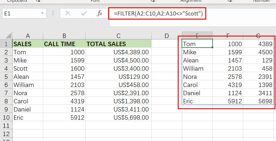
Take note that the filtered data on the right side of the figure above does not include any of Scott ‘s rows/calls.

 Example 5: How to use the date filter in Excel

---

Filtering in Excel by a date may be accomplished in a few different methods, which I will demonstrate below. If you attempt to put a date into the FILTER function in the same way that you would typically type into a cell, the formula will fail to operate properly.

Therefore, you may either enter the date you want to filter into a cell and then reference that cell in your formula… Alternatively,  you may use the DATE function.

When filtering by date, the same operators (>, =, etc…) are available as they are in other FILTER function applications. Each individual day/date in Excel is merely a number that has been formatted differently. In Excel, for example, the date “01/30/2022” is just the serial number “44591” formatted as a date. Each time you add a day to the calendar, this number increases by one… For example, “44591” “44592” “44593”

Thus, if one date is farther in the future, it might be regarded “greater than” another. In contrast, if one date is farther in the past, it might be considered to be “less than” another.

In this example, we’ll use a cell reference to filter on a date. This is identical to the example discussed in Example 2, except that we are dealing with dates instead of percentages.

Consider the following scenario: we want to filter a list of students, their exam results, and the dates on which the tests were administered… and we wish to display only tests conducted before to June (05/01/2022).

=FILTER(A2:C10, C2:C10 <G1)

Example 6: Filtering by date in Excel

---

In this example of date filtering in Excel, we’ll use the same data as in the previous one and attempt to obtain the same results… however, instead of referencing a cell, we’ll utilize the DATE function, which allows you to put the date straight into the FILTER function.

When using the DATE function to provide a date, you must first input the year, followed by the month and finally the day… each denoted with a comma (shown below).

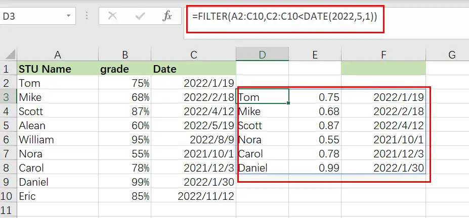
The assignment: Display only exams given before to May

The reasoning: Filter the range A2:C10 so that C2:C10 is less than or equal to the date (05/01/2022).

The following formula: In this example, the formula below is typed in the cell (D3).

=FILTER(A2:C10,C2:C10<DATE(2022,5,1))

Example 7: Filtering based on two Conditions

---

When utilizing the Excel FILTER function, you may want to produce data that fits many criteria. I’ll demonstrate two methods for filtering by several criteria in Excel, depending on the scenario and the desired behavior of the calculation.

The conventional method of adding another condition to your filter function (as shown by the Excel formula syntax) allows you to provide a second condition, where both the first AND second conditions must be fulfilled in order for the filter output to be returned.

However, I will demonstrate how to make a little tweak to the function so that you may choose to return/display in the filter function’s output/destination a second condition where EITHER condition might be satisfied. (To utilize AND logic, separate the conditions with an asterisk, or use a plus symbol to separate the criteria.)

In this example, we’re going to filter a collection of data and show those rows that satisfy BOTH the first and second conditions.

To utilize a second condition in this manner (using AND logic), just insert it after the first condition in the formula, separated by an asterisk (*). Each condition must be included in a separate pair of parentheses.

When a filter formula is used with several conditions, the columns referenced in each condition must be distinct.

In this case, we’d want to filter a list of clients based on their payment status and region… and to display those customers who are both current members AND paid on their payment status.

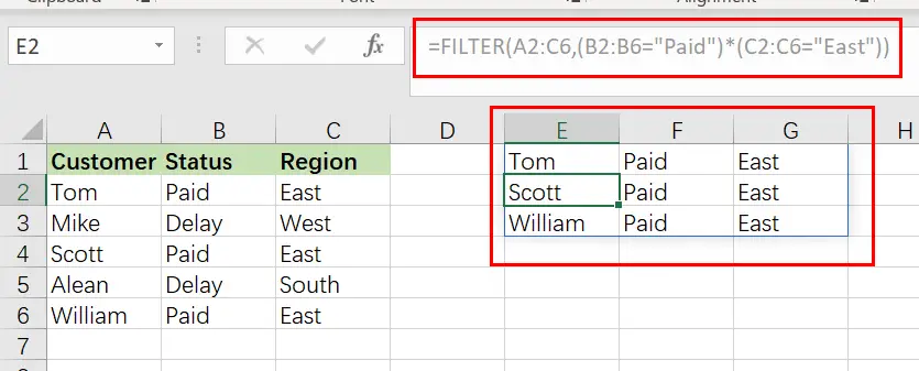
The objective is to provide a list of customers who are paid on payments, but only those who are in East region.

The reasoning: Filter the range A2:C6 such that B2:B6 equals the text “Paid,” AND C2:C6 equals the text “East“.

The following formula: In this example, the formula below is typed in the blue cell (E1).

=FILTER(A2:C6,( B2:B6="Paid")*( C2:C6 ="East"))

Example 8: Filtering Based on Two Conditions using OR Logic

---

In this example, we’re going to filter a collection of data and show those rows that satisfy either the first OR the second criterion.

To utilize a second condition in this manner (using OR logic), just insert it after the first condition in the formula, separated by a plus sign. Each condition must be included in a separate pair of parentheses (shown below).

When used in this manner, the FILTER formula allows you to choose criteria from the same or separate columns.

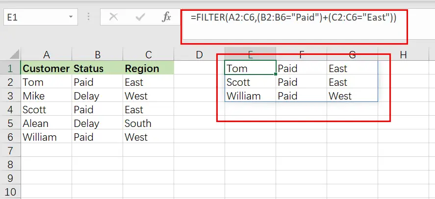
In this case, we’re filtering the same customer data as in the previous example, but this time we’re displaying a list of customers who either are in East region OR have paid on a payment. This will generate a list of clients to whom a payment notification have paid… whether they are current members or east region who have paid on their last payment.

The objective is to provide a list of customers who are in East region, as well as customers who have paid on payments regardless of whether they are in East region.

The following formula: In this example, the formula below is typed in the cell (E1).

=FILTER(A2:C6, (B2:B6="Paid ")+(C2:C6=" East ")

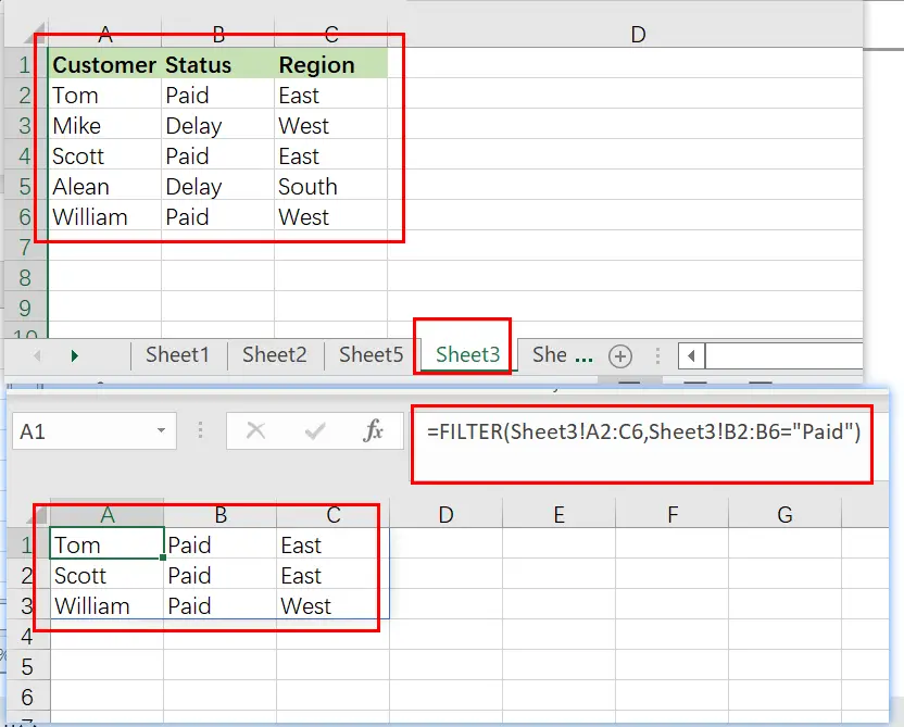
Example 9: Filter Data in Excel from Another Sheet

---

You may often encounter instances in Excel when you need to filter data from another sheet, where your raw unfiltered data is on one tab and your filter formula is on another sheet.

This may be accomplished by simply referring to a certain sheet’s name when providing the filter’s ranges. Thus, while you would typically give a range such as “A1:B4,” when referring another sheet when filtering, you indicate the sheet name by preceding the range with the sheet name and an exclamation mark, as in “SheetName!A1:B4“.

However, if the sheet name contains a space, an apostrophe must be used before and after the sheet name, as in "Sheet Name!" A1:B4.

The following is an example of how to filter data in Excel from a separate sheet, where the filter formula is located on a different sheet than the source range.

Consider the following scenario: On one sheet, you have a list of customers and their payment status, and you wish to present a filtered list of  paid customer on another sheet.

The job is to filter the list of customers on the Sheet3 and to display a separate list of customer names with a pay status on another worksheet.

The reasoning: Filter the range using the Sheet3‘ command! A2:C6, where ‘ Sheet3′ is the range! B2:B6 corresponds to the phrase “Paid“.

The following formula: In this example, the formula below is typed in the cell (A3).

=FILTER(Sheet3! A2:C6, Sheet3!B2:B6="Paid")

Example 10: Providing Maximum Number of Rows of Filtered Data

---

If your FILTER formula provides a large number of rows but your worksheet is restricted in space and you are unable to erase the data below, you may limit the amount of rows returned by the FILTER function.

Let us demonstrate how it works using a simple formula that filter data that grade is less than 0.7 from filter value in Cell F1:

=FILTER(A2:C10, B2:B10<F1)

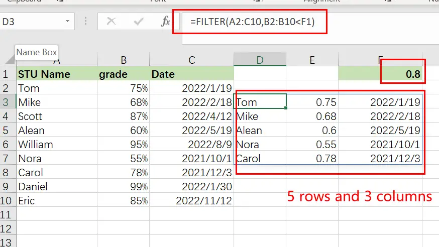
The preceding formula produces all records that it discovers, in this instance five rows. However, imagine you only have room for two. To output just the first two rows discovered, follow these steps:

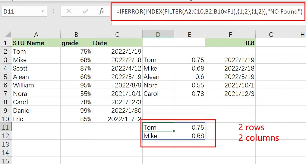
Step1: Incorporate the FILTER formula into the INDEX function’s array parameter

Step2: Use a vertical array constant such as 1;2 as the row num input to INDEX. It specifies the number of rows to return (2 in our case).

Step3: Use a horizontal array constant such as 1,2 for the column num parameter. It defines the columns that should be returned (the first 2 columns in this example).

Step4: To account for any mistakes caused by the absence of data meeting your criteria, you may wrap your calculation in the IFERROR function.

The entire excel filter formula is as follows:

=IFERROR(INDEX(FILTER(A2:C10, B2:B10<F1), {1;2},{1,2}), "No Found")

Conclusion

---

This section discusses the FILTER function and its many uses. In general, when it comes to time management, we need this feature for a variety of reasons. I demonstrated various techniques with accompanying examples, however there might be countless further iterations based on a variety of circumstances. If you know of another way to use this function, please share it with us.

---

• Excel IFERROR function
  The Excel IFERROR function returns an alternate value you specify if a formula results in an error, or returns the result of the formula.The syntax of the IFERROR function is as below:= IFERROR (value, value_if_error)….
• Excel INDEX function
  The Excel INDEX function returns a value from a table based on the index (row number and column number)The INDEX function is a build-in function in Microsoft Excel and it is categorized as a Lookup and Reference Function.The syntax of the INDEX function is as below:= INDEX (array, row_num,[column_num])…